DEPARTMENT OF ECONOMICS
COLLEGE OF BUSINESS AND ECONOMICS
UNIVERSITY OF CANTERBURY
CHRISTCHURCH, NEW ZEALAND
Long memory or shifting means?
A new approach and application to realised
volatility
by
William Rea, Les Oxley, Marco Reale, and Eduardo Mendes
WORKING PAPER
No. 04/2008
Department of Economics
College of Business and Economics
University of Canterbury
Private Bag 4800, Christchurch
New Zealand
Long memory or shifting means?
A new approach and application to realised
volatility
William Rea
1, Les Oxley
2, Marco Reale
1, and Eduardo Mendes
21. Department of Mathematics and Statistics,
2. Department of Economics
University of Canterbury
Private Bag 4800
Christchurch
New Zealand
May 22, 2008
AbstractIt is now recognised that long memory and structural change can be confused because the statistical properties of times series of lengths typical of financial and econometric series are similar for both models. We pro-pose a new set of methods aimed at distinguishing between long memory and structural change. The approach, which utilises the computational efficient methods based upon Atheoretical Regression Trees (ART), es-tablishes through simulation the bivariate distribution of the fractional integration parameter,d, with regime length for simulated fractionally
in-tegrated series. This bivariate distribution is then compared with the data for the time series. We also combine ART with the established goodness of fit test for long memory series due to Beran. We apply these methods to the realized volatility series of 16 stocks in the Dow Jones Industrial Average. We show that in these series the value of the fractional integra-tion parameter is not constant with time. The mathematical consequence
of this is that the definition ofH self-similarity is violated. We present
evidence that these series have structural breaks.
Keywords: Long-range dependence, strong dependence, global dependence, Hurst phenomena. JEL code C22.
Author’s Footnote: William Rea is Ph.D. candidate, Department of Mathematics and Statistics, University of Canterbury. Les Oxley is Professor, Department of Economics, Uni-versity of Canterbury. Marco Reale is Senior Lecturer, Department of Mathematics and Statistics, University of Canterbury. Eduardo Mendes is research assistant, Department of Economics, University of Canterbury. The authors thank Sir Clive Granger and Peter Robin-son for helpful conversations, Arek Ohanissian, Jeffrey Russell, and Ruey Tsay for providing us the source code for their test, and Marcel Scharth and Marcelo Medeiros for providing us with a copy of their realized volatility data.
1
Introduction
Long memory and fractionally integrated processes were introduced to the phys-ical sciences by, amongst others, Hurst (1951, 1957), and into the econometrics literature by Granger and Joyeux (1980). A major problem that arises, however, is that long memory and structural change are easily confused. As Sibbertsen (2004) states, it is often the case that structural break detection and location techniques report breaks when only long memory is present; similarly, long memory measurement techniques often report long memory when only struc-tural breaks are present even when the series are Markovian.
Section 3.6 of Banerjee and Urga (2005) Overview to the Journal of Econo-metrics, special issue on Structural breaks, long memory and stock market volatility, notes the potential confusion of ‘stochastic regime switching and long memory’ and cites a sample of the empirical literature in this area (Baum et al. (1999), Bos et al. (1999), and Hyung and Franses (2001, 2002)). However, the Diebold and Inoue (2001) conclusion that “. . .it would be na¨ıve to jump to the conclusion that structural change produces spurious inferences of long memory - even if the ‘truth’ is structural change, long memory might be a ‘con-venient shorthand and be very useful for prediction . . . ‘structural change’ and ‘long memory’ are effectively different labels for the same phenomenon, in which case attempts to label one as ‘true’ and the other as ‘spurious’ may be of
du-bious value”, seems to have led most researchers to ignore the issue of ‘model
confusion’. In effect Diebold and Inoue (2001) seem to propose, ‘it doesn’t re-ally matter what you call it.’ Unlike the literature on unit roots v. structural change, where it has been shown that persistence tests are severely compro-mised when the time series are characterized by breaks, to date, it has simply been too difficult to distinguish between long memory and structural change. There exist econometric examples which highlight long memory v. structural breaks, for example Smith (2005) and Ohanissian et al. (2008), but the over-whelming impression one gets from the literature is that ‘financial data exhibit long memory with a d (around) 0.4’ and if this is ‘spurious’ it doesn’t much matter.
The starting point of this paper is to argue that it does matter what you call it, especially if you are trying to model the pricing of financial assets for example, options and derivatives. The implications of assuming long range dependency and persistence versus short memory will have significant effects on the theoretical underpinnings of the markets where, empirically, long memory ‘appears’ to be most prevalent, financial markets. Secondly, we propose a fast method to identify breaks and to ascertain whether they are spurious - the practical problems of labeling the underlying process can now be ascertained.
The remainder of the paper is organized as follows. In Section (2) the properties of two models commonly applied across long memory series; i) frac-tional Gaussian noise and fracfrac-tionally integrated series and ii) constrained non-stationary series are presented. Section (3) outlines the empirical problem. In Section (4) the issue of why it matters whether we have ‘structural change’ or ‘long memory’ is presented using both statistical and finance theory arguments. Section (5) presents a method and related techniques that can i) quickly lo-cate potential breaks in a series and ii) test whether breaks so identified are spurious. The fast technique proposed here uses Atheoretical Regression Trees (ART) developed by Cappelli et al. (2008). Section (6) describes the data.
Sec-tion (7) presents some empirical examples using these methods by applying it to a dataset of realized volatilities and returns of 16 Dow Jones Industrial Average index stocks. Section (8) contains the discussion, and Section (9) gives final concluding remarks. A concise discussion of ART is given in Appendix (A).
2
Models
A number of models have been proposed to account for the extraordinary per-sistence of the correlations across time found in long memory series. Some have enjoyed considerable success in specific fields such as the Granger (1980) aggregation model in econometrics.
There are two common sets of models applied across long-memory series from diverse fields. One set are true long memory models, in particular, the Frac-tional Gaussian Noises (FGN) and FracFrac-tionally Integrated (FI(d)) processes. The other set are models which are non-stationary, but mean reverting. For simplicity the types of non-stationary models studied are ones in which the time series can be broken in a series of “regimes” within which it is a reasonable assumption that the mean is stationary. Two examples are structural break and Markov switching models.
2.1
Fractional Gaussian Noises and Fractionally Integrated
Series
Fractional Gaussian Noises (FGNs) were introduced into applied statistics by Mandelbrot and van Ness (1968) and are the stationary increments of an Gaus-sianH-self-similar stochastic process.
Definition 1 A real-valued stochastic process {Z(t)}t∈R is self-similar with indexH >0 if, for anya >0,
{Z(at)}t∈R=d{aHZ(t)}t∈R
where Rdenotes the real numbers and =d denotes equality of the finite
dimensional distributions. H is also known as the Hurst parameter. Definition 2 A real-valued process Z ={Z(t)}t∈R has stationary increments
if, for allh∈ R
{Z(t+h)−Z(h)}t∈R=d{Z(t)−Z(0)}t∈R.
It follows from Definition 1 thatH is constant for all subseries of anH -self-similar process.
FGNs are a continuous time process. Independently Granger and Joyeux (1980) and Hosking (1981) obtained the discrete time counter-parts to FGNs, the Fractionally Integrated processes (FI(d)).
FI(d)s are also a generalization of the “integration” part of the Box-Jenkins ARIMA (p,d,q) (AutoRegressive Integrated Moving Average) models to non-integer values of the integration parameter,d. Denoting the backshift operator
by B, the operator (1−B)d can be expanded as a Maclaurin series into an
infinite order AR representation (1−B)dXt= ∞ X k=0 Γ(k−d) Γ(k+ 1)Γ(−d)Xt−k =ǫt (1) where Γ(·) is the gamma function, and ǫt is an shock term drawn from an
N(0, σ2) distribution. The operator in Equation (1) can also be inverted and written in an infinite order MA representation. The two parameters H and d
are related by the simple formulad=H−1/2.
ARIMA models with non-integerdare known as AutoRegressive Fractionally Integrated Moving Average (ARFIMA) models. The AR(p) and MA(q) param-eters in ARFIMA models may be used to model any additional short-range dependence present in the series. Both FGNs and FI(d)s have been extensively studied. See the volumes by Beran (1994), Embrechts and Maejima (2002), and Palma (2007) and the collections of Doukhan et al. (2003) and Robinson (2003) and the references therein.
2.2
Constrained Non-Stationary Models
Klemes (1974) argued that long memory in hydrological time series was a sta-tistical artifact caused by analysing non-stationarity time series with stasta-tistical tools which assume stationarity. Often series which display the long memory property are constrained for physical reasons to lie in a bounded range. But beyond that we have no reason to believe that they are stationary. For example, in the series we study in this paper (realized volatilities, see Section 6), as long as the companies remain in the index their stock price volatilities cannot have an unbounded increasing or decreasing trend.
Models of this type which have been proposed typically have stochastic shifts in the mean, but overall are mean reverting about some long term average.
We define the break model as follows:
µyt= p X i=1
Iti−1≤t<tiµi (2)
where µyt is the mean of the time series,It∈S is an indicator variable which is
1 only ift∈S,t is the time,ti, i= 1, . . . , p, are the breakpoints andµi is the
mean of the regime i. In this case, a regime is defined as the period between breakpoints.
It is important to note that Equation (2) is just a way to represent a sequence of different models (i.e. models subjected to structural breaks). This model only deals with breaks in mean. It can be generalized for any kind of break. We are considering this class of model because it has been used by others when studying long memory processes. However, given a true break each regime must be modeled separately.
3
Model Confusion – The Empirical Problem
Despite the obvious theoretical differences between the FGNs or FI(d)s and constrained non-stationary models, they are difficult, if not impossible, to tell
apart in real data (Granger and Hyung (2004), Diebold and Inoue (2001)). As indicated earlier the difficulty is enough that Diebold and Inoue (2001) suggest ‘. . . in the sorts of circumstances studied in this paper, “structural change” and “long-memory” are effectively different labels for the same phenomenon . . . ’.
A number of authors have attempted to develop statistical tests to distin-guish between true long memory and other types of processes displaying sta-tistical long memory. Beran (1992) proposed a goodness-of-fit test for FGNs and ARFIMA models by comparing the estimated spectrum for the data with the theoretical spectrum of an FGN or ARFIMA with the specified parameters. The null hypothesis is that the times series is an FGN or ARFIMA. Rejection of the null does not lead to a clear alternative. Beran and Terrin (1996, 1999) de-veloped a test for which the null hypothesis is that theH parameter is constant in an FGN. As a constant H is fundamental to the definition of an FGN, the Beran and Terrin (1996, 1999) test could be considered to distinguish between a FGN and a multifractal as in multifractals theH (ord) parameter is allowed to change over time. Teverovsky and Taqqu (1999) proposed a procedure based on comparing the variance plots from the aggregated variance estimator with the differenced variance estimator which allows the researcher to distinguish be-tween long memory on the one hand and shifting means or deterministic trends on the other. The null is that the process is an FGN with no level shifts or deterministic trends. The alternative is that either level shifts or deterministic trends or both are present in the data but, the test provides no further informa-tion on their number or locainforma-tion. Smith (2005) modified the GPH estimator to discriminate between infrequent level shifts and long memory. The robustified estimator should return an estimate of d close to zero if there are only level shifts in the data. Ohanissian et al. (2008) developed a test of self-similarity based on different levels of aggregation of the series which cleverly avoids the issue of having to estimate any breaks or additional short memory correlation. The null hypothesis is thatdis constant at all levels of aggregation as required by the definition of an FI(d) process, hence the series is a true FI(d) series. Rejection of the null does not lead to a clear alternative.
Our procedures, outlined in Section (5), add to this literature by approaching the problem from the direction of explicitly modeling the breaks and is motivated by the following considerations.
As mentioned above, the use of structural break detection and location meth-ods are regarded as problematic because they tend to report breaks in FGNs and FI(d) series even though the data generating process is uniform throughout. For example, Wright (1998) proved that when the standard cumulative summa-tion (CUSUM) test, formalized by Brown et al. (1975), for detecting structural breaks was applied to long memory series the probability of finding a break converged to one with increasing series length.
We note that if a series is generated by a true long memory process, di-viding the series into a number of “regimes” of differing lengths through the use of a structural break location method will only yield subsamples of a single population. However, if, in fact, the series contains structural breaks, using a structural break location method will instead divide the series into a number of subpopulations. In the former case oura prioriexpectation is that the subsam-ples will have the same statistical properties as the full series. In the latter case the data generating process has one or more discontinuities. Consequently the statistical properties of the regimes will need to be individually estimated.
Despite this risk of model misspecification we could find no empirical study of the statistical properties of the “regimes” in simulated FGNs or FI(d) series of finite sample size when they were incorrectly analyzed by applying struc-tural break location methods to them. The use of ART (see Cappelli and Reale (2005), Rea et al. (2006), Cappelli et al. (2007), and Cappelli et al. (2008)), a computationally very fast structural break method, has allowed large scale sim-ulation studies to proceed which would have been computationally impractical with established techniques such as that due to Bai and Perron (1998, 2003).
4
Why it matters
The economics of why highly efficient financial markets would exhibit long range dependence is never addressed in the literature perhaps because it seems the econometric evidence is ‘overwhelmingly in favor of such a phenomenon’ or fol-lowing Diebold and Inoue (2001), the issue is purely semantic. Mikosch and Starica (2000) conclude “we have tried hard to find in the literature any con-vincing rational/economic argument in favor of long range dependent station-ary log returns, but did not find any.” As Ohanissian et al. (2008) also state, “the introduction of fractional components into volatility models is purely from an empirical perspective without any theoretical justification.” There is, how-ever, both a finance theory and regulator interest in long versus short memory modeling implications. As Jambee and Los (2005) highlight, the US Financial Accounting Standards Board (FASB), has an interest in how to value options because the traditional Black-Scholes formula is (for some reason) ‘not doing its job’.
Taylor (2000) analyses and simulates the consequences of a long memory assumption about volatility by comparing the implied volatilities for option prices based upon short and long memory volatility processes. In his analysis, the assumption of long memory has a significant effect upon the term struc-ture of implied volatilities and a relatively minor impact upon ‘smile effects’. Taylor’s approach was to simulate both long and short memory GARCH spec-ifications and derive the Black-Scholes implied volatilities from the resulting option prices. In particular, long memory term structures of the implied volatil-ity for an “at-the-money” option have much more variety in their shape than those based upon short memory assumptions; they may also imply ‘kinks’ for short maturity options and may not have a monotonic shape. In addition, long memory assumptions can lead to implied term structures on different valuation dates that sometimes intersect. Long memory term structures do not converge rapidly to a limit as the lifetime of the option increases and it is difficult to estimate the limit for the typical value of d=0.4. None of these outcomes occur in a short memory specification of his models. In a related approach, Bollerslev and Mikkelson (1996) simulate call option prices for the Standard & Poor’s 500 composite index and show that, as one might expect, the price of a call option is much higher when long memory in the volatilities is assumed compared to when it is not.
Ohanissian et al. (2008) is complementary to Taylor (2000), but in their case they consider three affine models; a short memory; a switching mean for volatility between high and low state which is the process to introduce ‘spurious’ long memory; and a fractional stochastic volatility model (true long memory).
Using a simulation approach they examine the mis-pricings that occur from using the ‘wrong’ model. The main finding of their paper is that: “ignoring or mis-specifying the nature of observed long memory characteristics in volatility leads to serious option mispricing. Specifically when the true DGP is spurious long memory, using either a no long memory model or a true long memory model leads to general underpricing of call options, by as much as two-thirds. On the other hand when the DGP is true long memory, using either a no long memory or a spurious long memory leads in general to overpricing of call options.” These mispricings extend out to the entire horizon they consider which is two years.
Jambee and Los (2005) demonstrate that the standard Black-Scholes op-tion pricing formula must assume the Hurst exponent is exactly equal to 0.5, otherwise the expiration time-adjusted variance of the stock rate of return will not be constant (as assumed elsewhere by Black and Scholes). As Jambee and Los (2005) further argue, the fact that the S&P500 has an H=2/3 and a shape (Zolatarev) exponent of 3/2 (implying that the variance of the distribution is therefore non-existing or infinite) strongly suggests that “the Index is statisti-cally unsuitable as an ‘underlying’ index for option valuation, despite the fact it is traded on the Chicago Board of Trade”. Likewise options written in anti-persistent markets, for example some foreign exchange markets (where H=0.25 and the Zolatarev shape exponent is 4), again, according to Jambee and Los (2005), “don’t make sense, even though they are traded on the Philadelphia Stock Exchange”. One must conclude, therefore, that the degree of persistence does have a significant impact on option values via the time dependent volatility and thus the risk-neutral probabilities used in their valuation.
Consider now some statistical/econometric issues around the pricing of op-tions when volatility is stochastic and has short memory. Here the modeling commences with separate diffusion specifications for the asset prices and its volatility such that option prices then depend on several parameters including a volatility risk premium and the correlation between the differentials of the Wiener processes in the separate diffusions. Duan (1995) provides an explicit option valuation framework for a GARCH (1,1) process with short memory. Comte and Renault (1998) and Bollerslev and Mikkelson (1996, 1999) describe methods to price options when volatility has a long memory. Here, they re-place the Wiener process in the volatility equation with fractional Brownian motion. However, their option pricing formula requires independence between the Wiener process in the price equation and the volatility process which is inconsistent with the empirical evidence on stock returns. Furthermore, ap-plication of the theory of option pricing when volatility follows a discrete-time ARCH process with fractional integration requires approximation because the fundamental filter is an infinite order polynomial that must be truncated at some power N. Option prices will therefore be sensitive to the truncation point and large values and long price histories from an assumed stationary process are required.
Sibbertsen (2004) reiterates that long memory appears important when con-sidering the volatilities of stock returns and as a consequence, the valuation of options and derivatives, etc. In this literature, the dominant empirical approach is the ARCH-type class of models which assume that the conditional variance de-pends on the currently known information and crucially do not allow long-range dependence. Empirically, however, it would seem that shocks to the conditional variance decay slower than ARCH-type modeling would posit. Assumptions
about long-range dependence are crucial for optimal forecasts of the variance and more generally for asset price valuation, as a consequence, it is important to know whether long memory or short memory (with infrequent shifts) is the ‘true’ model. Sibbertsen (2004) concludes that apparent long memory in UK, Canada, Japan and USA GNP, is mainly due to ‘structural breaks in the data’. Martens et al. (2004) propose a nonlinear model for realized volatilities that ‘simultaneously captures long memory, leverage effects, volatility persistence that depends on the size of the shocks, structural breaks and day of the week effects’. They conclude that level shifts in the S&P 500 volatility do not ac-count for the long memory feature - the fractional integration parameter does decline when explicitly modeling the structural break, but remains significantly different from zero. However, in their example they ‘find it difficult to pin-down exactly when the level shift occurred and it is most adequately characterized as a gradual increase in volatility during 1996-1997.’ They consider an alternative of multiple breaks following Andreou and Ghysels (2002), but do not identify them explicitly, instead they allow for gradual level shifts using a fifth-order polynomial in t. They reject a logistic function that changes monotonically from 0 to 1 as t increases as ‘too restrictive as it only allows for a single struc-tural change in the level.’ As a consequence they do not provide a convincing case that they have actually identified the ‘correct location(s)’ of the breaks and hence their conclusion appears overly strong.
Mikosch and Starica (1999) find structural change in asset return dynamics and argue it is responsible for evidence of long memory. Moreover, Mikosch and Starica (2000) argue that the IGARCH model and LRD are incompatible, “if the IGARCH model is the generating process of the log-returns, the LRD effect has nothing to do with LRD; it is simply an artifact since the sample ACFs do not measure anything.”
It therefore seems important, both for aspects of finance theory, econometric modeling and empirical consistency that we try to identify whether the data are generated by ’true’ long memory processes.
5
Method
A fast structural break location technique called Atheoretical Regression Trees (ART) was recently introduced by Cappelli and Reale (2005). ART is based on least squares regression trees (LSRT) which are widely used, see Breiman et al. (1993) for a detailed description. An Atheoretical Regression Tree is a non-parametric approach used to find breaks in the level of a stochastic process. This method exploits, in the framework of LSRTs, the contiguity property introduced by Fisher (1958) for grouping a single real variable into maximally homogeneous groups. See the appendix for an discussion of ART.
In this paper we present two different procedures for distinguishing between real and spurious breaks based on ART. The first is fast, the second is very slow but has greater sensitivity than the first. In both procedures the null hypothesis is that the series is an FI(d). The alternative is that the series has one or more structural breaks.
i) Numerical – ART with Beran (1992) Test 1. Estimatedfor the full series.
2. Estimate goodness of fit of thisdvalue with the Beran (1992) test. 3. Apply ART to the series to obtain the candidate break points. 4. Estimatedfor each regime reported by ART.
5. Apply the Beran (1992) test to each regime twice. Once using das esti-mated for the full series and once usingdas estimated for the regime. 6. Assess whetherdis constant across series. Details of how the assessment
was made are given in Section (7).
ii) Graphical – Using ART to estimate the bivariate distribution ofdwith regime length.
1. Estimatedfor the full series.
2. Estimate goodness of fit of thisdvalue with the Beran (1992) test. 3. Through simulation obtain the bivariate probability distribution ofdwith
regime length.
(a) Simulate a large number of FI(d) series with the samed and series length as the series under test.
(b) Use ART to break the series into “regimes”. (c) Estimatedwithin these regimes.
(d) Calculate the empirical median, 75%, 95%, and 99% confidence in-tervals.
(e) Plot the bivariate distribution.
4. Apply ART to the full series to obtain the candidate break points. 5. Estimatedfor each regime reported by ART.
6. For each regime overplot the d estimate and regime length on the previ-ously determined empirical distribution.
7. Assess whetherdis constant. Details of how the assessment was made are given in Section (7).
In step 3a of the Graphical method we found that typically it was neces-sary to simulate 10,000 to 25,000 FI(d) series to obtain a good estimate of the bivariate distribution.
Unless otherwise stated alldestimates were obtained using the estimator of Haslett and Raftery (1989) as implemented by in in theRsoftware (R Develop-ment Core Team (2005)) packagefracdiffof Fraley et al. (2006). The Beran test was evaluated using functions implemented in longmemo of Beran et al. (2006). FI(d) series were simulated with the functionfarimaSiminfSeriesof Wuertz (2005). The implementation of the Whittle available to us sometimes exited with an error when trying to estimatedin short regimes so was not used. The graphical procedure can also be used to assess whether the mean, stan-dard deviation, skewness, and kurtosis are constant.
0 500 1000 1500 2000 2500 −1 0 1 2 3 4
Realized Volitilities of AIG with Breaks Points
Observation
Log Volitility
1 2 3 4 5 6
Figure 1: AIG realized volatility series plot with breaks identified by ART.
6
The Data Set
The data set comprised the realized volatility of 16 Dow Jones Industrial Av-erage (DJIA) index stocks and were provided by Scharth and Medeiros (2007). The 16 stocks are Alcoa (AA), American International Group (AIG), Boeing (BA), Caterpillar (CAT), General Electric (GE), Hewlett Packard (HP), IBM, Intel (INTC), Johnson and Johnson (JNJ), Coca-Cola (KO), Merck (MRK), Pfizer (PFE), Wal-Mart (WMT), and Exxon (XON). The period of analysis was from January 3, 1994 to December 31, 2003. Trading days with abnor-mally small trading were excluded, leaving a total of 2539 daily observations. The daily realized volatility was estimated using the two time scale estimator of Zhang et al. (2005) with five-minute grids, which is a consistent estimator of the daily volatility. A fuller explanation of the dataset and how the realized volatil-ities were calculated can be found in Scharth and Medeiros (2007). It should be noted that because all 16 are part of the DJIA they cannot be considered to be independent series.
In this paper we will give detailed results for American International Group (AIG) and, where practical, state the results for the other 15 stocks. Figure (1) presents a plot of the data with the breakpoints reported by ART marked as vertical dashed lines. Figure (2) presents the autocorrelation function and a spectral estimate. The ACF and spectral estimate are typical of long memory time series. A visual examination of these diagnostic plots for all 16 series suggested they were all of the long memory type.
0 100 200 300 400 500 0.0 0.2 0.4 0.6 0.8 1.0
Lag in Trading Days
ACF
(A) ACF of AIG Realized Volatilities
0.0 0.1 0.2 0.3 0.4 0.5 0.05 0.10 0.20 0.50 1.00 2.00 5.00 20.00 frequency spectrum
(B) Spectral Estimate of AIG Realized Volatilities
bandwidth = 0.000686
Figure 2: (A) ACF of AIG realized volatility series. (B) Spectral estimate obtained using modified Daniell smoothers.
7
Results
7.1
d
Estimates
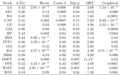
Both procedures begin with the estimation of dand a Beran (1992) goodness of fit test of the full series. These two results are presented in Columns “d Est” and “Beran” of Table (1) respectively. As reported by other authorities a d
estimate close to 0.4 is appropriate for most series. Realized volatilities usually present a long memory behavior and a visual examination of the series, ACF and periodogram suggests all 16 series are of the long memory type. However, for 11 of the series (AA, BA, CAT, GE, HP, IBM, INTC, KO, MSFT, PFE and WMT) the null hypothesis of an FI(d) withdestimated from the data was not accepted at a level of 5%.
7.2
Numerical – ART with Beran Test
Next, we apply ART to the full series. Figure (1) presents the breakpoints in graphical from superimposed on the plot of the data. Column “Period” of Table (2) presents the range of trading days which form each regime. The first line is the full series, the subsequent lines are the regimes.
We then estimatedand perform two Beran tests for each regime. For AIG column “d Est” of Table (2) reports the destimates, column “d=0.40” reports the goodness of fit using the series d estimate, column “d=d(t)” reports the goodness of fit using the within regimedestimates.
There are two ways to interpret the data in Table (2). The first is to examine the regimes for which the Beran test fails to accept the null hypothesis when the value ofdis held at the series value (column “dEst” of Table 2). We then check
Stock d Est Beran Constd Imp p ORT Graphical AA 0.42 2.65×10⁻⁶ 0.006 0.03 2.68 1.54×10⁻⁵ AIG 0.40 0.14 0.009 0.04 4.02 0.068 BA 0.40 0.02 0.10 0.18 1.63 0.0001 CAT 0.41 0.002 0.0007 0.15 5.32 6.02×10⁻⁶ GE 0.44 0.04 0.008 0.11 4.98 3.32×10⁻⁵ GM 0.36 0.09 0.34 0.03 5.20 0.0004 HP 0.44 0.002 0.04 0.04 0.50 0.004 IBM 0.44 8.93×10⁻⁶ 0.02 0.05 1.13 0.02 INTC 0.46 3.59×10⁻⁷ 0.03 0.30 2.20 0.03 JNJ 0.40 0.16 0.46 0.04 3.62 0.02 KO 0.42 2.57×10⁻⁶ 0.02 0.04 4.40 3.74×10⁻¹⁰ MRK 0.39 0.34 0.06 0.03 3.89 0.006 MSFT 0.46 0.008 0.43 0.007 11.24∗ 0.02 PFE 0.42 4.43×10⁻⁶ 0.43 0.007 3.88 0.0001 WMT 0.42 2.95×10⁻¹² 0.02 0.007 4.15 0.001 XON 0.44 0.09 0.04 0.04 1.26 0.004
Table 1: For the 16 stocks in the sample column “d Est.” reportsdas estimated by the Haslett and Raftery (1989) estimator. Column “Beran” reports the p-value returned by the goodness-of-fit test of Beran (1992) applied to the full series. Column “Constd” reports the p-value obtained when the Beran (1992) test was used to test if d within the regimes reported by ART were different from dfor the full series. Column “Imp p” reports the p-value obtained when the number of times the Beran test showed an improved fit by using the regime
destimate instead of the seriesdestimate was used. Column “ORT” is the test statistic from the method of Ohanissian et al. (2008) a single asterisk (∗) marks the result which was significant at the 0.05 level. Column “Graphical” reports the p-value the graphical technique for testing for a constantdpresented in this paper was used.
whether the null hypothesis is accepted ifdis set to the value as estimated for that regime.
In the case of AIG, the series could be adequately modeled by an FI(0.4) process as the Beran test reported a p-value of 0.14, which indicated the null should not be rejected. When we applied this method of evaluating if d is constant to the data, the first regime reported by ART was clearly anomalous. The Beran test reported a p-value of 0.003, indicating a clear non-acceptance of the null, if the regime was tested against the seriesdestimate. However, when the first regime was tested against the within regimedestimate (d= 0.25) the Beran p-value was 0.54. This clearly indicated an FI(0.25) model provided a better fit for the first regime.
Thus for AIG, ART had located a structural break in the data at the first breakpoint.
If we count the number of regimes for which the null of the series being an FI(d), with das estimated for the full series, is not accepted at either the five or one percent levels and use a simple binomial distribution, we can assign a conservative p-value to the null hypothesis of true long memory. These p-values are listed in column “Constd” of Table (1). As can be seen, for the constantd
approach, the null was not accepted for 11 of the 16 stocks.
Alternatively we could use the data from Table (3) and estimate the proba-bility that the number of regimes showing an improved fit were due to chance. Table (3) represents the empirically determined distribution of improvement in fit as reported by the Beran test when using the within regimedestimate rather than the full series destimate for 1000 simulated FI(0.4) series. In the case of AIG an improved fit was reported for all seven regimes.
A simple approach to assess whether the changes in p-values for AIG are the result of a better fit or simply random events is to assume that changes in p-value are distributed binomially. We can then calculate the probability of seven improvements being a random event.
The p-values for this variation of the Numerical method are presented in column “Impp” of Table (1) for all 16 stocks. As can be seen, for the improved
p-value approach the null hypothesis was not accepted for 12 of the 16 stocks.
7.3
Graphical – Bivariate Distribution of
d
with Regime
Length
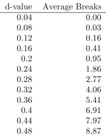
The Graphical method differs from the Numerical method in that it establishes through simulation the empirical bivariate distribution of regime length and d
estimate for FI(d) series. As noted earlier structural break methodologies tend to report breaks in FI(d) series where no breaks exist. Table (4) presents the mean number of breaks reported by ART in 1000 replications of 2500 data point FI(d) series with differentdvalues. For financial data wheredis typically about 0.4 ART reports, on average, about seven breaks in a simulated 2500 data point series. All of these breaks are spurious as the data generating process is uniform throughout the series.
A simple alternative model which has been well studied is the two-state Markov switching model, see for example Smith (2005). We compared the empirical bivariate distribution of estimateddagainst regime length for a two-state Markov switching model with seven switches with FI(0.4) series.
Period dEst d= 0.40 d=d(t) 1-2539 0.40 0.14 -1-1168 0.25 0.003 0.54 1169-1854 0.36 0.35 0.46 1855-1944 0.30 0.62 0.73 1945-2146 0.37 0.76 0.79 2147-2250 0.35 0.38 0.39 2251-2414 0.33 0.43 0.62 2415-2539 0.27 0.81 0.85
Table 2: Column “Period” is the period under test in trading days from the beginning of the sample. Column “dEst” reports the d estimates for the full series and the regimes reported by ART. Column “d = 0.40” reports the p-value returned by the Beran (1992) test fordas estimated for the series. Column “d=d(t)” reports the p-value returned by the Beran (1992) test for the regimes of AIG realized volatilities.
Result Percentage Mean Change
Improvement 63.8 0.068
Same or Worse 36.2 -0.079
Table 3: Percentages of “regimes” for which the Beran (1992) yielded an im-provement in fit if the regime estimate ofH was used instead of the series value in simulated FGNs.
d-value Average Breaks
0.04 0.00 0.08 0.03 0.12 0.16 0.16 0.41 0.2 0.95 0.24 1.86 0.28 2.77 0.32 4.06 0.36 5.41 0.4 6.91 0.44 7.97 0.48 8.87
Table 4: Average number of breaks report by ART in a 2500 data point series for simulated FI(d) series different values ofd.
0 500 1000 1500 2000 2500 0 0.1 0.2 0.3 0.4 0.5 0 5 10 15 Regime Length
(A) d Estimates for Seven Break Markov Series
d Estimate Percentage of Regimes 0 500 1000 1500 2000 2500 0 0.1 0.2 0.3 0.4 0.5 0 5 10 15 Regime Length
(B) d Estimates for FI(0.40) Series
d Estimate
Percentage of Regimes
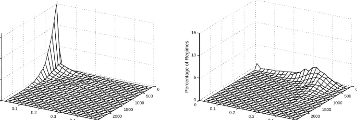
Figure 3: (A) Bivariate distribution of d estimates with regime length for a 2500 data point Markov switching series with seven switches. (B) Bivariate distribution ofdestimates with regime length for FI(0.40) series.
Panel A of Figure (3) presents the empirically estimated bivariate distribu-tion from 1000 replicadistribu-tions of the two-state Markov switching series with eight regimes (i.e. seven switches) and 2500 data points. Panel B presents the results for the 1000 FI(0.4) series.
The bivariate distribution for the Markov switching series reflected the fact that there was no long memory in these series despite the fact that the Haslett-Raftery estimator reported a mean value of d= 0.29 for 1000 replications. In general, ART correctly located the switchpoints and hence divided the series into regimes consisting of nothing more than random numbers with the same mean. The Haslett-Raftery estimator was then applied to these regimes and it correctly reported a d value of zero or close to zero. For the FI(0.4) series, splitting the series up into “regimes” with ART did not mask the fact that the series had long memory.
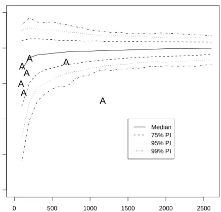
The results for AIG are presented in Figure (4). As we are interested in whether d has changed, the figure presents the empirical conditional bivariate distribution of dgiven regime length when the null hypothesis of FI(0.4) was known to be true. The solid and three sets of dashed lines present the empirically determined median, 75%, 95% and 99% confidence intervals. The “A” symbols represent the seven AIG data points. This method automatically took account of the problem that the Haslett-Raftery estimator was biased in short series, which is seen in Figure (4). Visual inspection of this graph shows the 1168 trading day regime (right most “A” in Figure 4) has a statistically significant
d value to the full series. Again, we can use a simple binomial distribution to obtain a conservative p-value of whether the null is likely to be true.
Column “Graphical” of Table (1) presents the calculated p-values for this method for all sixteen stocks. As can be seen, the null hypothesis is not accepted for 15 of the 16 stocks. The null hypothesis was not rejected for AIG. The calculation of thepvalue took no account of how far the points were outside the empirical confidence intervals. A visual inspection of Figure (4) suggests the null hypothesis would not be accepted for AIG if a more sophisticated calculation
0 500 1000 1500 2000 2500 0.0 0.1 0.2 0.3 0.4 0.5
d Estimates AIG and FI(d) d=0.40
Length of Regime d value
A
A
A
A
A
A
A
Median 75% PI 95% PI 99% PIFigure 4: Conditional bivariate distribution ofdgiven regime length. The AIG regimes are represented with the symbol “A”.
was carried out.
7.4
Comparisons with Other Tests and Procedures
For comparison purposes we present two alternative views of the data; the new test of Ohanissian et al. (2008) and rolling window estimates ofdsuch as those used by Cajueiro and Tabak (2005).
The results for the new test of Ohanissian et al. (2008) are presented in column “ORT” of Table (1). The Ohanissian et al. (2008) test only rejects the null of a FI(d) for the MSFT stock. We believe the reason for the lack of rejections to be a consequence of their choice of the GPH estimator. Their test appears soundly based in theory. In practice, for series of the length we are dealing with either the Haslett-Raftery or Whittle estimators would be more suitable.
It is not possible to obtain an estimate fordat a point. The best that can be done is to estimate d in some data window about the point for which we
Event Approximate Date No. of Series with Break
Asian Financial Crisis 1 Aug 1997 4
Russian Financial Crisis 20 Jul 1998 11
Brazilian Financial Crisis 13 Jan 1999 1
NASDAQ Peak 3 Mar 2000 9
Terrorist Attacks 11 Sep 2001 3
DJIA 4-year low 9 Oct 2002 11
Table 5: Six major events identified by Scharth and Medeiros (2007) as having an effect on stock market volatility and how many series show a structural break near these dates.
want to know the value ofd. Panels A and B in Figure (5) present the results of the rolling d estimates using two window sizes as reported by ART for the AIG data. The 1168 trading day window reported in Panel A was the length of the first regime. The evidence from this rolling window supports the results of our two new procedures which reported thatdis not constant. The lowestd
reported for any 1168 trading day period is the first regime reported by ART. In panel (B) a 202 trading day window was used. This is the length of the third regime reported by ART and has the highest estimated within-regime
d value. The locations of the ART breakpoints are marked and labeled one through six. It is curious that breakpoints 1, 2, 4, and 6 are at sharp changes in thed estimate. One should not over interpret this as there are other sharp changes for which ART did not report a break and two breakpoints (3 and 5) which do not correspond to a sharp change ind.
Panel C of Figure (5) presents thedestimates for the same two data window sizes (202 and 1168 points) for a simulated multifractal with mean shifts which has eight regimes (seven breaks) alternating between 312 data points atd=0.15 and 313 data points atd=0.3 and with mean shifts of one standard deviation in terms of the input noise series. In for this particular series the 202 data point window was shorter than the regimes and hence at most the window included data from two regimes. The longer data window always covered parts of at least four regimes and does not reflect the series’ multifractal structure. The locations of the breaks are marked by dashed vertical lines and labeled 1 through 7. Panel D of Figure (5) presents the results for a simulated FI(d) series with
d=0.40 and the same two window sizes.
7.5
Higher Moments
In Section (5) we stated that the “Graphical” method could be applied to higher moments. Figure (6) presents the results of the estimates of the standard de-viations for AIG. Three of the AIG data points are below the 95% empirical confidence interval, two of which are well below the 99% empirical confidence interval. Thus for these three regimes the data is more homogeneous than ex-pected for an FI(d) series.
0.0 0.1 0.2 0.3 0.4 0.5
(A) Rolling 1168 Day d Estimates
AIG Median 95% CI
(B) Rolling 202 day d Estimates
1 2 3 4 5 6 AIG ART Breakpoints 0 500 1000 1500 2000 2500 0.0 0.1 0.2 0.3 0.4 0.5 (C) Multifractal d Estimates 1 2 3 4 5 6 7 202 Obs. 1168 Obs. Breaks 0 500 1000 1500 2000 2500 (D) FI(0.40) d Estimates d Estimate 202 Obs. 1168 Obs. Median 202 95% CI 1168 95% CI
Figure 5: Panels (A) and (B) rollingdestimates for window lengths 1168 and 202 trading days. Horizontal lines in panel (A) are the median and 95% confidence intervals for FI(0.4) series. The vertical dashed lines in panel (B) are locations of the ART break points. Panel (C) rolling estimates of d for the same two window lengths for a seven break multifractal (details in text) with breakpoints marked by dashed vertical lines. (D) a pure FI(0.40) series with two window lengths with median and 95% confidence intervals.
0 500 1000 1500 2000 2500 0.4 0.6 0.8 1.0 1.2
Std Devs. AIG and FI(0.40)
Regime Lengths Std Dev.
A
A
A
A
A
A
A
Median 75% PI 95% PI 99% PIFigure 6: Conditional bivariate distributions of standard deviation given regime length for simulated FI(0.40) series. The “A” symbols are the standard devia-tions of the AIG realized volatility series regimes.
7.6
Historical Events
Figure (1) shows the realized volatility series with each break identified. In their study of these same 16 series Scharth and Medeiros (2007) identified six events which appeared to have an impact on the volatility of the stocks. Some of these were close to instantaneous and their effects were felt immediately. Others were events which developed over time and whose effects were felt spread out over a longer time period.
Table (5) presents a list of these events and the number of series for which ART reported a break close to this time. The strongest event was the Russian financial crisis in which 11 of the 16 stocks showed a structural break within 12 trading days of 20 July 1998. AIG showed structural breaks for the Russian crisis, September 11 terrorist attacks and the DJIA low.
Individual stocks also had a number of other breaks. Some of these were related to known events which one would expect would only affect that stock and perhaps a very small number of related companies. For example the AIG stock shows a break at 9 April 2001. At this time there were talks between AIG and American General Corporation (AGC). In May 2001, AIG bought AGC for $US23 billion.
8
Discussion
In Section (3) we noted that when breaks are reported by a structural break lo-cation method in FI(d) series that they are fundamentally different from breaks reported in, say, a Markov switching series. Most of this paper has concentrated on analysing the long memory properties of the regimes, yet we recall that ART finds candidate breakpoints by detecting shifts in the mean. A change indand a shift in mean are only related if ART has located a genuine structural break in the series.
The results presented in Figure (3) showed that our intuition about the differences between the two types of breaks was indeed correct when our proce-dures are applied to simulated data. ART usually correctly located the switch points in the two state Markov switching series and thed estimator then cor-rectly returned an estimate of d of zero or close to zero for the regimes. The breaks reported by ART for the FI(d) series are different. They were caused by the long excursions away from the mean exhibited by FI(d) series. All of them are spurious. Consequently the d estimates in panel B of Figure 3 reflect the fractional integration of the whole series. These represent two extreme cases; series with mean switches but no other serial correlation and pure FI(d) series. The empirical evidence from Figures (1), (4), (5), and (6) and Table (2) all point to the first breakpoint being a genuine structural break. Historically this break was at the time of the Russian financial crisis.
As a parameter only has meaning in the context of a model, ifdis allowed to be a function of time, as demanded by the evidence, we are led to the so-called multifractal models. However, this leads to three problems. First, a time-varyingdnullifies one of the great strengths of the FI(d) models (or FGNs), namely that a single parameter can model the long-range dependence properties of the whole series. On a more technical level, a time-varyingd(orH) violates the definition of self-similarity. Once a time-varying d is admitted, then any
model for the data must of necessity be non-stationary.
Second, as far as we are aware, there are no estimators ofdwhich can handle a non-stationary d. All assume that d is stationary as required by the FI(d) model.
Third, there is the issue of interpretability. It has been difficult to interpret FI(d) series in terms of economic and financial processes generating the volatility data. Consider the implication of an increasingdas observed in the AIG data. An FI(d) model with constantdtells us that any given observation is correlated with all past states of the system into the infinite past. Ifdis allowed to increase, we have the strange situation where data points separated by longer periods of time are more strongly correlated than those separated by shorter periods of time.
Given the arguments of Klemes (1974) it seems reasonable to consider whether estimates of parameters which which were obtained by estimators which assume stationarity, such as those ford, have any meaning at all in these series.
The results presented in Figure (6) showed that in four cases the data within the regimes were more homogeneous than expected at the five percent level. This was further evidence that the mean shifts reported by ART were, in fact, real and not an artifact of incorrectly analysed FI(d) series.
While past literature claims FI(d) series model the long memory properties of financial data well, perhaps the most serious drawback to them is on a philo-sophical level. The breaks in FI(d) series reported by ART are the result of random fluctuations in the data generating process to which no further signifi-cance can be assigned. For AIG four of the six reported breaks are correlated with historical events for which a plausible cause and effect mechanism can be proposed.
In previous studies the use of the test of Beran (1992) has often been over-looked. It is a valuable tool in estimating the goodness of fit of real data to an FGN or ARFIMA(p,d,q) series. The d estimates presented in the second col-umn of Table (1) are comparable with estimates reported by other authorities for similar series. But what has not been previously reported was that often the fit to an FI(d) was poor with the null not being accepted for 11 of the 16 series in our data set. The results from our procedures point to dnot being constant coupled with mean shifts as a probable cause of the poor fit. For AIG all seven regimes can be adequately modeled by an FI(d) provided dis allowed to vary with time.
For comparison purposes we have provided two alternative views of the data used by other authorities.
First, we applied the new test of Ohanissian et al. (2008). These results are presented in the column labeled “ORT” in Table (1). We chose four levels of aggregation and the critical values for theχ2distribution with three degrees of freedom are 7.82 for p= 0.05 and 11.35 for p = 0.01. The results show only MSFT is not a true long memory process on the basis of the Ohanissian et al. (2008) test.
Second, we have used rolling estimates of d (see Figure 5). In previous literature there has been no way to determine where one might expect the value ofdto change or what length data window should be used. On both questions we have allowed the results of ART to guide us. The two different length data windows showed a statistically significant increase in d with time. The 202 trading day data window showed a distinct break in d estimate at the end of
the first regime as reported by ART and smaller changes at breakpoints 2, 4, and 6. These results lend some support the results of our new methodology. However, the use of rolling estimates of d appears less useful in determining wheredmay change compared to either of our two procedures.
9
Conclusions and Future Research
It is now well established that long memory and structural change are easily confused, however, most researchers, particularly in the financial econometrics area, choose to ignore the problem, or simply find it too difficult, empirically, to distinguish between them.
In this paper we firstly argued that ‘it does matter’ whether the data exhibit ‘true’ long memory using examples from the option pricing area. Taylor (2000), Mikosch and Starica (2000), Ohanissian et al. (2008), Jambee and Los (2005) and Bollerslev and Mikkelson (1996) all represent examples of ‘what can go wrong in the pricing’ if short memory (with possible breaks) is ‘confused’ with long memory. What you call it ‘does matter’. The second, and more important, contribution of the paper was to propose a new approach and related techniques that can quickly locate potential breaks in the series and test whether the breaks identified are spurious. This is a fundamentally different way to approach the problem of distinguishing between long memory and structural change and has not previously been proposed and complements the recent approaches proposed by for example, Ohanissian et al. (2008) and Smith (2005). The particular structural break-test method used here, based upon Atheoretical Regression Trees, is fast enough to be practical with the large sized datasets typical in the financial econometrics area. The new approach was then applied to sixteen financial data series to examine whether mean shifts and long memory were linked in realized volatility series. The data were also examined using some existing tests including that of Ohanissian et al. (2008).
This paper set out to examine whether mean shifts and long memory were linked in realized volatility series. In all sixteen series we were able to establish that link. However, as Martens et al. (2004) found, even after locating and taking account of the mean shifts thedparameter remains significantly different from zero. We also established that pure FI(d) series do not fit the observed bivariate distributions, a time-varying d is required. However, a time-varying
d presents serious unresolved statistical issues as we estimated a time varying parameter with tools which assume that parameter is constant.
The historical events associated with the ART break dates point to the fact that we have real structural breaks in these data.
The graphical method presented here of determining if d is not constant across the series was shown to be more sensitive to changes in d than using ART in conjunction with the Haslett and Raftery (1989) estimator and the test of Beran (1992). We believe the test could be improved through the use of the Whittle estimator.
Ultimately, however, we must admit that the hypothesis of Klemes (1974) that long memory was a statistical artifact caused by analyzing non-stationary time series with statistical tools that assumed stationarity, has not been fully established. We have established the existence of shifting means in the 16 time series examined in the paper. However, the resulting model(s) of their data
generating processes suggest a multifractal with mean shifts which embodies the notion of a time varying d, and hence creates its own statistical problems, both estimation and logical. As a consequence, given that FI(d) series are both stationary and linear, they may well be the ‘best’ approximation currently available for these type of data.
10
Acknowledgements
The authors would like to thank Sir Clive Granger and Peter Robinson for help-ful conversations, Arek Ohanissian, Jeffrey Russell, and Ruey Tsay for providing us the source code for their test, and Marcel Scharth and Marcelo Medeiros for providing us with a copy of their realized volatility data.
A
Appendix: Atheoretical Regression Trees
Time series data consists of a series of observations ordered by time. In the context of regression trees (RTs) time assumes the role of the predictor variable when, in fact, it is merely a counter. A common source of poor predictive perfor-mance in RTs is that the distribution of the response variable is not orthogonal to the predictor variables (see Fig 8.12 of Hastie et al. (2001) for an example). This problem does not arise in univariate time series. This gives us reason to suspect they will perform well in the location of structural breaks.
The model considered is:
yt=µg+ǫt, g= 1, . . . , G, t=Tg−1+ 1, . . . , Tg, (3)
where Gis the number of regimes (and G−1 the number of breakdates), yt
is the observed response variable and ǫt is the error term at time t (we adopt
the common convention thatT0= 0 andTG=T whereT is the series length).
This is a pure structural breaks model because all the model coefficients are subject to change and it has been employed by Bai and Perron (1998, 2003) to detect abrupt structural changes in the mean occurring at unknown dates. The problem is to estimate the set of breakdates (T1, . . . , Tg, . . . , TG−1) that define a partition of the series
P(G) ={(1, . . . , T1), . . . ,(Tg−1+ 1, . . . , Tg), . . . ,(TG−1+ 1, . . . , T)}, into homogeneous intervals such thatµg 6=µg+1. Bai and Perron (1998, 2003) propose an estimation method based on the least squares principle: for each
G-partition, the corresponding least square estimates of the µg’s are obtained
by minimizing the within-group sum of squares
W SSy|P(G)= G X g=1 Tg X t=Tg−1+1 (yt−µg)2. (4)
The estimated breakdates ( ˆT1, . . . ,Tˆg, . . . ,TˆG−1) are associated with the parti-tion P∗(G) such that P∗(G) = argmin
P(G)W SSy|P(G). In this approach, the breakdate estimators are global minimizers since the procedure considers all possible partitions by using the dynamic programming approach proposed by
Fisher’s (1958) to find the least squares partition ofT contiguous objects into
Ggroups. His efficient algorithm exploits the additivity of the sum of squares criterion using a dynamic programming approach Bellman and Dreyfus (1962) that applied to ordered data points finds the global minimum. Despite the computational saving, the method cannot deal with high values of T and G
and the same remark holds for the Bai & Perron’s procedure, even with today’s computing power.
In the case of time series data Hartigan (1975) provides an excellent jus-tification in favor of the (faster) binary division algorithm: suppose that the observed time series consists ofGsegments within each of which the values are constant, i.e. model (1) becomes a piecewise constant model withǫt= 0. Then,
there is a partition into Gsegments for which the within-group sum of squares is zero and it will be identified by a sequential splitting algorithm as the one in ART.
In other words, if the data have a hierarchical structure then ART will find the overall optimum, otherwise it provides a suboptimal solution for which, because the partitions are contiguous, misplacements can occur only on the boundaries. As discussed in Hansen (2001), although structural breaks are treated as immediate, it is more reasonable to think that they take a period of time to become effective, thus misplacements on the boundaries are not a concern.
Given that the global search algorithm requires O(n2) steps, whereas ART, at any tree node requires O(n(h)) steps to identify the best split, suboptimality does not appear a high price to pay.
References
Andreou, E. and Ghysels, E. (2002). Detecting multiple breaks in financial market volatility dynamics. Journal of Applied Econometrics, 17:579–600. Bai, J. and Perron, P. (1998). Estimating and Testing Linear Models with
Multiple Structural Changes. Econometrica, 66(1):47–78.
Bai, J. and Perron, P. (2003). Computation and Analysis of Multiple Structural Change Models. Journal of Applied Econometrics, 18:1–22.
Banerjee, A. and Urga, G. (2005). Modelling structural breaks, long memory and stock market volatility: an overview.Journal of Econometrics, 129:1–34. Baum, C. F., Barkoulas, J. T., and Caglayan, M. (1999). Long memory or structural breaks: can either explain nonstationary real exchanges rates under the current float. Journal of International Markets, Finance and Money, 9:359–376.
Bellman, R. E. and Dreyfus, S. E. (1962). Applied Dynamic Programming. Princeton University Press.
Beran, J. (1992). A Goodness-of-Fit Test for Time Series with Long Range Dependence. Journal of the Royal Statistical Society B, 54(3):749–760. Beran, J. (1994).Statistics for Long Memory Processes. Chapman & Hall/CRC
Beran, J. and Terrin, N. (1996). Testing for a change in the long-memory parameter. Biometrika, 83(3):627–638.
Beran, J. and Terrin, N. (1999). Testing for a change in the long-memory parameter. Biometrika, 86(1):233.
Beran, J., Whitcher, B., and Maechler, M. (2006). longmemo: Statistics for
Long-Memory Processes (Jan Beran) – Data and Functions. R package
ver-sion 0.9-3.
Bollerslev, T. and Mikkelson, H. (1996). Modeling and pricing long memory in stock marker volatility. Journal of Econometrics, 73:151–184.
Bollerslev, T. and Mikkelson, H. (1999). Long term equity anticipation securities and stock market volatility dynamics. Journal of Econometrics, 92:75–99. Bos, C., Franses, P. H., and Ooms, M. (1999). Long-memory and level shifts:
Re-analysing inflation rates. Empirical Economics, 24:427–449.
Breiman, L., Friedman, J., Olshen, R., and Stone, C. (1993). Classification and
Regression Trees. Chapman & Hall/CRC.
Brown, R. L., Durbin, J., and Evans, J. (1975). Techniques for Testing the Con-stancy of Regression Relationships over Time.Journal of the Royal Statistical
Society Series B, 37(2):149–192.
Cajueiro, D. O. and Tabak, B. M. (2005). Testing for time-varying long-range dependence in volatility for emerging markets. Physica A, 346:577–588. Cappelli, C., Penny, R. N., Rea, W. S., and Reale, M. (2008). Detecting
mul-tiple mean breaks at unknown points with Atheoretical Regression Trees.
Mathematics and Computers in Simulation. forthcoming.
Cappelli, C., Rea, W. S., and Reale, M. (2007). The Application of Regression Trees to the Detecting of Multiple Structural Breaks in the Mean of a Time Series. Research Report UCMSD 2007/4, Department of Mathematics and Statistics, University of Canterbury.
Cappelli, C. and Reale, M. (2005). Detecting Changes in Mean Levels with Atheoretical Regression Trees. Research Report UCMSD 2005/2, Department of Mathematics and Statistics, University of Canterbury.
Comte, F. and Renault, E. (1998). Long memory in continuous time stochastic volatility models. Mathematical Finance, 8:291–323.
Diebold, F. X. and Inoue, A. (2001). Long Memory and Regime Switching.
Journal of Econometrics, 105:131–159.
Doukhan, P., Oppenheim, G., and Taqqu, M. (2003). Theory and Applications
of Long-Range Dependence. Birkha¨user.
Duan, J.-C. (1995). The GARCH option pricing model. Mathematical Finance, 5:12–32.
Embrechts, P. and Maejima, M. (2002). Selfsimilar Processes. Princeton Uni-versity Press.
Fisher, W. D. (1958). On Grouping for Maximum Homogeneity.Journal of the
American Statistical Association, 53(284):789–798.
Fraley, C., Leisch, F., Maechler, M., Reisen, V., and Lemonte, A. (2006).
fracd-iff: Fractionally differenced ARIMA aka ARFIMA(p,d,q) models. R package
version 1.3-0.
Granger, C. W. J. (1980). Long Memory Relationships and the Aggregation of Dynamic Models. Journal of Econometrics, 14:227–238.
Granger, C. W. J. and Hyung, N. (2004). Occasional structural breaks and long memory with an application to the S&P 500 absolute stock returns. Journal
of Empirical Finance, 11:213–228.
Granger, C. W. J. and Joyeux, R. (1980). An Introduction to Long-range Time Series Models and Fractional Differencing. Journal of Time Series Analysis, 1:15–30.
Hansen, B. (2001). The New Econometrics of Structural Change: Dating Breaks in the US Labor Productivity. Journal of Economic Perspectives, 15(4):117– 128.
Hartigan, J. (1975). Clustering Algorithms. John Wiley and Sons.
Haslett, J. and Raftery, A. E. (1989). Space-time Modelling with Long-memory Dependence: Assessing Ireland’s Wind Power Resource (with Discussion).
Applied Statistics, 38(1):1–50.
Hastie, T., Tibshirani, R., and Friedman, J. (2001). The Elements of Statistical
Learning. Springer.
Hosking, J. R. M. (1981). Fractional Differencing. Biometrika, 68(1):165–176. Hurst, H. E. (1951). Long-term storage capacity of reservoirs. Transactions of
the American Society of Civil Engineers, 116:770–808.
Hurst, H. E. (1957). A suggested statistical model of some time series that occur in nature. Nature, 180:494.
Hyung, N. and Franses, P. H. (2001). Structural breaks and long memory in US inflation rates: Do they matter for forecasting? Research Report EI2001-13, Econometric Research Institute, University of Rotterdam.
Hyung, N. and Franses, P. H. (2002). Inflation rates, long memory, levels, shifts or both? Econometric Institute Report 2002-08, Erasmus University. Jambee, S. and Los, C. (2005). Long-memory options: Valuation. mimeo. Klemes, V. (1974). The Hurst phenomenon - a puzzle? Water Resources
Research, 10(4):675–688.
Mandelbrot, B. B. and van Ness, J. W. (1968). Fractional Brownian Motions, Fractional Noises and Applications. SIAM Review, 10(4):422–437.
Martens, M., van Dijk, D., and de Pooter, M. (2004). Modeling and Forecast-ing S&P 500 Volatility: Long Memory, Structural Breaks, and Nonlinear-ity. Tinbergen Institute Discussion Paper TI2004-067/4, Erasmus Universeit, Rotterdam and Tinbergen Institute.
Mikosch, T. and Starica, C. (1999). Change of structure in financial time se-ries, long-range dependence and the GARCH. Technical report, University of Groningen.
Mikosch, T. and Starica, C. (2000). Long range depedenence effects and ARCH modeling. Technical report, University of Groningen.
Ohanissian, A., Russell, J. R., and Tsay, R. S. (2008). True or Spurious Long-Memory? A New Test. Journal of Business and Economic Statistics, forth-coming.
Palma, W. (2007). Long-Memory Time Series Theory and Methods. Wiley-Interscience.
R Development Core Team (2005). R: A language and environment for
statis-tical computing. R Foundation for Statistical Computing, Vienna, Austria.
ISBN 3-900051-07-0.
Rea, W., Reale, M., Cappelli, C., and Brown, J. (2006). Identification of level shifts in stationary processes. In Newton, J., editor, Proceedings of the 21st
International Workshop on Statistical Modeling, pages 438–441. IDESCAT,
Galway.
Robinson, P. M. (2003). Time Series with Long Memory. Oxford University Press.
Scharth, M. and Medeiros, M. C. (2007). Asymmetric Effects and Long Memory in the Volitility of Dow Jones Stocks. working paper.
Sibbertsen, P. (2004). Long memory versus structural breaks: An overview.
Statistical Papers, 45(4):465–515.
Smith, A. D. (2005). Level Shift and the Illusion of Long Memory in Economic Time Series. Journal of Business and Economic Statistics, 23(3):321–335. Taylor, S. J. (2000). Consequences for option pricing of a long memory in
volatility. mimeo.
Teverovsky, V. and Taqqu, M. (1999). Testing for Long-Range Dependence in the Presence of Shifting Means or a Slowly Declining Trend, Using a Variance-Type Estimator. Journal of Time Series Analysis, 18(3):279–304.
Wright, J. H. (1998). Testing for a Structural Break at Unknown Date with Long-Memory Disturbances.Journal of Time Series Analysis, 19(3):369–376. Wuertz, D. (2005). fSeries: Financial Software Collection. R package version
220.10063.
Zhang, L., Mykland, P., and A¨ıt-Sahalia, Y. (2005). A Tale of Two Time Scales: Determining Integrated Volatility with Noisy High-Frequency Date. Journal