SparseHC: a memory-efficient
online hierarchical clustering algorithm
Thuy-Diem Nguyen
1, Bertil Schmidt
2, and Chee-Keong Kwoh
3 1 School of Computer Engineering, Nanyang Technological University, Singapore2 Institut f¨ur Informatik, Johannes Gutenberg University, Mainz, Germany
3 School of Computer Engineering, Nanyang Technological University, Singapore
Abstract
Computing a hierarchical clustering of objects from a pairwise distance matrix is an im-portant algorithmic kernel in computational science. Since the storage of this matrix requires quadratic space with respect to the number of objects, the design of memory-efficient approaches is of high importance to this research area. In this paper, we address this problem by presenting a memory-efficient online hierarchical clustering algorithm called SparseHC. SparseHC scans a sorted and possibly sparse distance matrix chunk-by-chunk. Meanwhile, a dendrogram is built by merging cluster pairs as and when the distance between them is determined to be the small-est among all remaining cluster pairs. The key insight used is that for finding the cluster pair with the smallest distance, it is unnecessary to complete the computation of all cluster pairwise distances. Partial information can be utilized to calculate a lower bound on cluster pairwise distances that are subsequently used for cluster distance comparison. Our experimental re-sults show that SparseHC achieves a linear empirical memory complexity, which is a significant improvement compared to existing algorithms.
Keywords: hierarchical clustering, memory-efficient clustering, sparse matrix, online algorithms
1
Introduction
Clustering is an important unsupervised machine learning technique to group similar objects in order to uncover the inherent structure of a given dataset. Depending on the output, clustering algorithms are broadly divided into two main categories: hierarchical clustering and partitional (or flat) clustering [2, 12, 26]. The structured output produced by hierarchical clustering algo-rithms is often more informative than the unstructured set of clusters returned by partitional clustering algorithms [16, 24]. Thus, hierarchical clustering is a crucial data analysis tool in many fields including computational biology and social sciences [9]. Nonetheless, the quadratic time and especially the quadratic memory complexity have limited the use of hierarchical clus-tering software to rather small datasets [24]. Since many areas of computational science face a
Volume 29, 2014, Pages 8–19
ICCS 2014. 14th International Conference on Computational Science
8 Selection and peer-review under responsibility of the Scientific Programme Committee of ICCS 2014
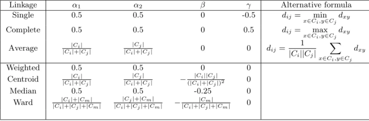
Table 1: The parameters of the Lance-Williams recurrence formula for 7 popular linkage schemes
Linkage α1 α2 β γ Alternative formula
Single 0.5 0.5 0 -0.5 dij= min x∈Ci,y∈Cjdxy Complete 0.5 0.5 0 0.5 dij= max x∈Ci,y∈Cjdxy Average |Ci| |Ci|+|Cj| |Cj| |Ci|+|Cj| 0 0 dij= 1 |Ci||Cj| x∈Ci,y∈Cj dxy Weighted 0.5 0.5 0 0 Centroid |Ci| |Ci|+|Cj| |Cj| |Ci|+|Cj| − |Ci||Cj| (|Ci|+|Cj|)2 0 Median 0.5 0.5 -0.25 0 Ward |Ci|+|Cm| |Ci|+|Cj|+|Cm| |Cj|+|Cm| |Ci|+|Cj|+|Cm| −|Ci|+||CCjm|+||Cm| 0
data explosion, addressing the problem of computing a hierarchical clustering from a large and possibly sparse pairwise distance matrix in a memory-efficient way is becoming increasingly important. In this paper, we tackle this problem by presenting a new general-purpose online hierarchical clustering algorithm called SparseHC.
Hierarchical clustering can be divided into two categories: the agglomerative “bottom-up” approach and the divisive “top-down” approach [24]. We focus on the former category: ag-glomerative hierarchical clustering (AHC). AHC algorithms can be characterized as sequential, agglomerative, hierarchical, and non-overlapping [7, 23]. In AHC algorithms, objects or data points are first treated as singletons and subsequently merged one pair of clusters at a time until there is only one cluster left. There are seven commonly used linkage schemes: single, complete, average (UPGMA), weighted (WPGMA), centroid (UPGMC), median (WPGMC) and Ward’s method. The properties of each scheme are discussed in [8]. The merging criteria used by all these schemes can be neatly represented with the recurrence formula by Lance and Williams [14]. Given that two clustersCi andCj have previously been merged into clusterCk,
the distance between clusterCk and any unmerged clusterCm is defined as:
dkm=d(Ci∪Cj, Cm) =α1dim+α2djm+βdij+γ|dim−djm|
The specific parameters for each scheme are defined in Table 1.
Depending on the input data, AHC algorithms can be divided into the “stored data ap-proach” and the “stored matrix apap-proach” [1, 18]. The stored data approach requires the recalculation of pairwise distance values for each merging step. Since only data points are stored in the main memory, algorithms in this approach can achieve O(N) space complexity often at the expense of O(N3) time complexity [19], where N is the number of input data points. One notable algorithm in the stored data approach is the nearest- neighbor chain al-gorithm, which achieves O(N) space complexity and O(N2) time complexity for the Ward’s method linkage scheme. However, this algorithm is not applicable to the centroid and me-dian linkage schemes because these schemes do not fulfill the required reducibility criterion i.e. d(Ci∪Cj, Cm) ≥min(d(Ci, Cm), d(Cj, Cm)) [18, 19]. For the single-, complete- and
average-linkage schemes, this algorithm requires O(N2) space and time complexity [10]. On the con-trary, in the stored matrix approach an all-against-all pairwise distance matrix of size N2 is first computed and then used for clustering. As a result, this approach requires O(N2) time and memory complexity [26].
To overcome the low memory efficiency of classical AHC algorithms, new techniques perform either data reduction by random sampling (e.g. data sampling and partitioning in CURE [11])
or data summarization by using a new data structure to represent the original data (e.g. the CF tree in BIRCH [27]). Although these algorithms have linear memory complexity [26], the dendrograms produced by these algorithms are indeterministic and are dissimilar those produced by standard AHC tools because of the random procedures being used.
In this paper, we focus on reducing the primary memory consumption of the AHC stored matrix approach. We introduce SparseHC, a general-purpose memory-efficient AHC algorithm for single-, complete- and average-linkage schemes. SparseHC is an online algorithm. Borodin and El-Yaniv [5] defined online algorithms as algorithms that focus on scenarios where “the input is given one piece at a time and upon receiving an input, the algorithm must take an irreversible action without the knowledge of future inputs”. Because online algorithms only require partial input in the main memory for processing, they are often used to target problems with high space complexity. To our knowledge, there are only a few existing online hierarchical clustering algorithms for the stored matrix approach including MCUPGMA [15] for the average scheme and ESPRIThcluster [25] for single and complete schemes.
SparseHC employs a similar strategy as in MCUPGMA and hcluster where the input dis-tance matrix is first sorted and then processed in a chunk-by-chunk manner. SparseHC incor-porates two new techniques in order to achieve significantly better performance:
1. Compression of the information in the currently loaded chunk of the input matrix into the most compact form.
2. Usage of an efficient graph representation to store unmerged cluster connections, which allows constant access to these connections for faster speed.
2
Background and Concepts
SparseHC and other online AHC algorithms work based on the observation that once the values of an input distance matrix are sorted in ascending order and loaded chunk-by-chunk from the top, the merge order and the dendrogram distances can be accurately determined using only the loaded part i.e. without any knowledge about the unseen portion.
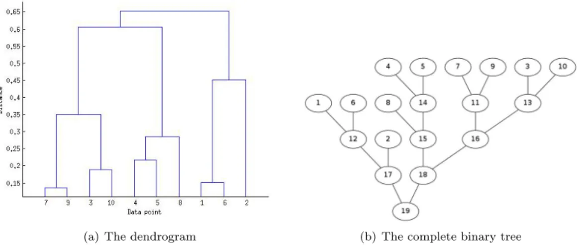
(a) The dendrogram (b) The complete binary tree
Figure 1: Illustration of the dendrogram and the corresponding complete binary tree produced by applying average-linkage clustering to a full distance matrix computed from 10 data points. SparseHC takes a sorted distance matrix D as input and iteratively builds a dendrogram
from reading only a part of D in each iteration step as shown in Figure 1. Depending on the available main memory, a sequence of values 0 =λ0 < λ1 < . . . < λT =θ is built on-the-fly.
In each iteration step 1 ≤t ≤ T, all distances dxy with λt−1 ≤ dxy < λt are read from D.
Starting from the a tree consisting of onlyN leaves where a leaf nodei(1≤i≤N) represents the singleton cluster Ci ={i}, a binary tree (which is the dendrogram) is built from bottom
up. Since only two clusters are merged at a time, the full binary tree has a height ofN−1 and consists of 2N−1 nodes (see Figure 1).
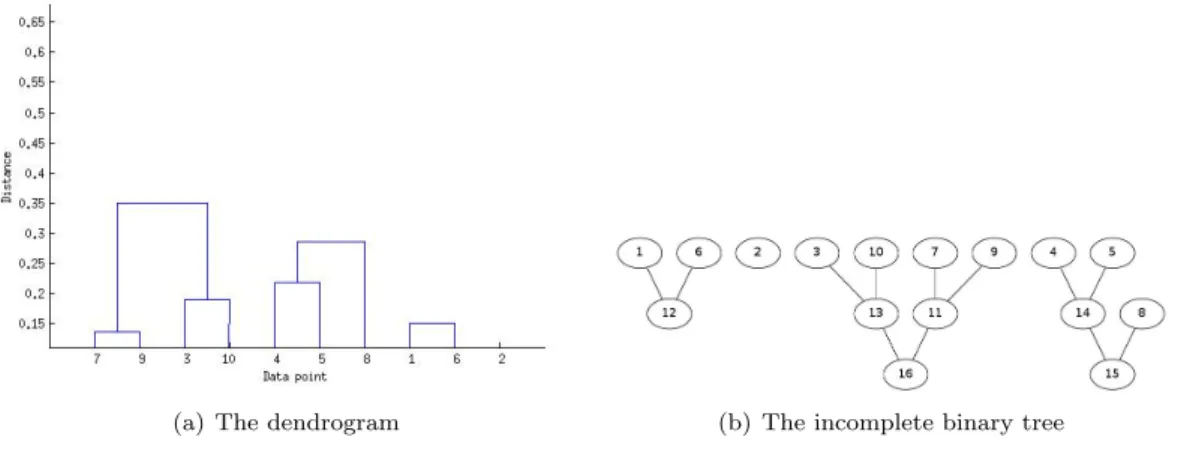
In offline AHC algorithms,D has to be a full pairwise distance matrix. However, in online AHC algorithms such as SparseHC, D can be either full or sparse. A sparse distance matrix Dθ uses a predefined distance cutoff θ (0 ≤ θ < 1) and stores only distance values up to θ
(0≤dxy≤θ,∀dxy∈D). For sparse matrix clustering, the output dendrogram has a height in
the range of [1, N−1] and a size in the range of [N,2N−1] as shown in Figure 2.
(a) The dendrogram (b) The incomplete binary tree
Figure 2: Illustration of the dendrogram and the corresponding incomplete binary tree produced by applying average-linkage clustering to a sparse distance matrix computed from 10 data points with a distance cutoffθ= 0.4.
The input to SparseHC is a sorted full or sparse distance matrix stored in a list of tu-ples (i, j, dij) format (similar to the MATLAB sparse matrix external format: http://www. mathworks.com/help/matlab/ref/spconvert.html). The maximum element of a full matrix is 1.0 while that of a partial matrix is a pre-defined distance cutoff θ < 1.0. The ability to process sparse distance matrices is particularly useful in applications like taxonomic studies in bioinformatics [4, 25] where only the lower part of the final dendrogram is of interest. In these situations, runtime and memory usage are further reduced depending on the sparsity of the input matrix. The memory efficiency and ability of SparseHC to process sparse matrices come at the cost of pre-sorting the input matrices. Nonetheless, the memory performance of SparseHC is not affected if an external merge sort algorithm [13] is used for the sorting stage.
Similar to offline AHC algorithms, during the clustering process, SparseHC needs to store all the connections amongst unmerged clusters to figure out which cluster pair will be merged next. However, same as other online AHC algorithms, SparseHC only stores the connections amongst active clusters. A cluster pair is calledactivein iteration steptwhen (1) both clusters do not have a parent and (2) at least one distance value between the member data points has been read from the input file during the firstt iteration steps. We observe that active clusters contribute to only a small subset of unmerged clusters. The memory efficiency of online AHC algorithms is determined by their ability to store active connections in a compact way.
Table 2: The time and memory complexity of different graph representations. We derive the adjacency map from the adjacency list to facilitate edge operations required by SparseHC.
Representation Storage Add edge Remove Edge Query edge Incidence matrix O(|V||E|) O(|V||E|) O(|V||E|) O(E)
Adjacency matrix O(|V|2) O(1) O(1) O(1)
Incidence list O(|V|+|E|) O(1) O(E) O(E) Adjacency list O(|V|+|E|) O(1) O(E) O(V)
Adjacency map O(|V|+|E|) O(1) O(1) O(1)
Table 3: Distancedij between clusterCi andCj for clustering sparse matrices
Linkage Edge definition Cluster distance Complete condition
Incomplete edge Complete edge
Single e(ijt)= () d(ijt)= 1.0 d(ijt)=dxy n(ijt)= 1 Complete e(ijt)= (nij(t)) d(ijt)= 1.0 dij(t)=dxy nij(t)=|Ci||Cj| Average e(ijt)= (sij(t), n(ijt)) d(t) ij = s(ijt)+λ(t)(|Ci||Cj|−n(t) ij) |Ci||Cj| d (t) ij = s(ijt) |Ci||Cj| n (t) ij =|Ci||Cj|
In SparseHC, we use an undirected weighted graph to model the connections amongst active cluster pairs. This graph consists of a set of verticesV and a set of edgesE. The vertices are the nodes of the binary tree i.e. V ={C1, C2, . . . , C2N−1}. SparseHC uses a fixed size array
to store all possible vertices, hence allowing O(1) vertex query and update. The undirected weighted edges are the active connections amongst the clusters.
Graphs are typically implemented using an adjacency matrix, an adjacency list, an incidence matrix or an incidence list [21]. The time and space complexity of each representation are shown in Table 2. To facilitate its cluster merging process, SparseHC prefers a graph representation that requires minimum storage for the graph and allows constant time to perform edge insertion, edge deletion, and edge update. Therefore, we have modified the standard adjacency list to assist these operations. We call this graph representation the adjacency (hash) map. The adjacency map is a collection of unordered hash maps, one for each vertex of the graph. Each hash map records the set of neighbors of its vertex using the neighbor vertex identification number as the key. Because of this adjacency map representation, SparseHC can useO(|V|+|E|) space to store all the clusters and their active connections. More importantly, these connections can be accessed and updated inO(1) time.
3
SparseHC
3.1
Algorithm
The definition of the edgee(ijt)between two active clustersCiandCjin iteration steptis defined
in Table 3 depending on the clustering scheme. d(ijt)is the minimum possible distance between
Ci and Cj and is computed according to Table 3. sij(t) (n(ijt)) is the sum (number) of distance
values between any member ofCi to any member ofCj that has been read from the input file
so far. λt is the maximum distance value loaded from the input matrix so far.
In each iteration stept, active edges are partitioned into two sets: a set ofcomplete edgesK(t) and a set ofincomplete edges I(t)(both sets are stored in the adjacency map). A complete edge is a connection between two active clusters that are ready to be merged. An incomplete edge is
a connection between two active clusters that are yet to be merged. For complete- and average-linkage schemes, an edge is complete whenn(ijt)=|Ci||Cj|. Otherwise, whenn(ijt)<|Ci||Cj|, the
edge is considered incomplete. For single-linkage scheme, an edge is complete whenn(ijt) = 1
i.e. the connection between two clusters is complete as soon as the first distance value between any member reads has been read from the input.
Let min(I(t)) (min(K(t))) denote the smallest distance value inI(t) (K(t)). The high-level description of the SparseHC algorithm in each iterationt (1≤t≤T) consists of three steps:
1. Read the distance valuesdxy from matrixD in ascending order until the adjacency map
is full and determine the value λ(t).
2. Update/create the edges for all active cluster pairs with the new distances and partition them intoI(t)andK(t).
3. Retrieve the edgee(ijt) for whichd(ijt)= min(K(t))≤min(I(t)). Merge the cluster pair Ci
andCj into clusterCk. Deleteeij(t)fromK(t)and combine existing edges to either cluster
Ci orCj into new edges to clusterCk. Repeat until min(K(t))>min(I(t)).
Algorithm 1 shows the details of SparseHC.
3.2
Correctness
To show the dendrogram produced by SparseHC is correct, we need to prove that up to the distance cutoffθboth the merge distance values and the merge order are preserved.
Merge distances: Let d(ijt)be the merge distance between two clusters Ci andCj assuming
that they are being merged by SparseHC in an iteration t. Let dij be the merge distance
betweenCiandCjproduced by a traditional AHC algorithm. We need to show thatd(ijt)=dij.
Indeed, whenCi andCj are merged by SparseHC, the edge e(ijt) is complete. By definitions of
dij in Table 1 and in d(ijt)when eij(t)is complete in Table 3, it holds that d(ijt)=dij. Therefore,
the merge distance values are preserved.
Merge order: To prove that SparseHC preserves the merge order, we show that ifCiandCj
are merged beforeCk andCm, thendij ≤dkm. At the time whenCiandCj are being merged
in an iteration t, we have d(ijt)=dij = min(K(t)). In stept, after Ci and Cj are merged, the
status of the edgee(kmt) is one of the followings:
1. e(kmt) is active and complete⇒e(kmt) ∈K(t). For a complete edge, it holds thatd(kmt) =dkm.
Besides,e(kmt) ∈K(t)⇒min(K(t))≤d(kmt). Therefore,dij ≤dkm
2. e(kmt) is active and incomplete⇒e( t)
km∈I(t). For an incomplete edge, it holds that d( t)
km≤
dkm. In SparseHC, it always holds that min(K(t))≤min(I(t))⇒dij ≤min(I(t)).
Besides,e(kmt) ∈I(t)⇒min(I(t))≤d(kmt). Therefore,dij ≤dkm
3. e(kmt) is inactive⇒e( t)
km∈ {/ K(t)∪I(t)}. For an inactive edge, it holds thatλt< d( t)
km≤dkm.
SinceCi andCj have been merged in iterationt, dij ≤λt. Therefore,dij < dkm
For all cases, we haved(ijt)=dij anddij≤dkmi.e. both the merge distances and the merge
order are preserved in SparseHC.
3.3
Memory efficiency
While standard offline AHC algorithms store all the connections amongst unmerged clusters in memory (i.e. |Ci| × |Cj| values for a cluster pair Ci, Cj), SparseHC uses at most two values
Algorithm 1SparseHC algorithm for a sorted input matrix D fromN data points stored as a list of tuples (x, y, dxy).
Ci ← {i} ∀i= 1, . . . , N
E.max size←N {E is the adjacency mapE=K∪I}
k←N;t←0;λ0←0{initialize cluster idk, iterationt, distance thresholdλ}
whileD=∅do t←t+ 1
whileD=∅and E.size ≤E.max sizedo dxy←D.get next();D=D\ {dxy}
Ci←Cx.get ancestor();Cj←Cy.get ancestor()
e(ijt).update(dxy){createe(ijt)if it does not exist}
computed(ijt) {use the cluster distance formula in Table 3}
if e(ijt) is completethen
Ci.minK←min(Ci.minK,dij(t));Ci.merge candidate←Cj
else
Ci.minI ←min(Ci.minI,d(ijt))
end if end while
λt←dxy {λtis the largest distance in an iteration}
whiledij= min(K(t))≤min(I(t))andk≤2N−1do
k←k+ 1; Ck ←Ci∪Cj {merge clustersCiand Cj into clusterCk}
for allCmsuch thate(imt) ∈E∨e(jmt) ∈Edo
e(kmt) ←merge(e( t) im, e(jmt)){s(kmt) ←s( t) im+s(jmt); n(kmt) ←n( t) im+n(jmt)} E=E∪ {e(kmt)} \ {eim(t), e(jmt), e(ijt)}
computed(kmt) {use the cluster distance formula in Table 3}
if e(kmt) is completethen
Ck.minK←min(Ck.minK,dkm(t));Ck.merge candidate←Cm
else
Ck.minI←min(Ci.minI,d(kmt))
end if end for end while
if E.size ≥E.max sizethen
E.max size←2×E.max size{dynamically increase the adjacency map size} if E.size ≥RAM.size then
return partial result{when the memory limit is reached} end if
end if end while return full result
per cluster pair: the number of connections n(ijt) and the sum of distances s(ijt) (see Table 3).
Specifically, SparseHC maintains only one value per cluster pair (n(ijt)) for complete-linkage
clustering, two values per pair (n(ijt), s(ijt)) for average-linkage clustering and none for
single-linkage clustering.
Compared to offline AHC tools, SparseHC uses less primary memory because of two reasons: (1) SparseHC stores only the information from the currently loaded chunks and (2) It stores a compact version of the seen information: at most two values per active cluster pair.
Compared to existing online AHC tools such as hcluster and MCUPGMA, SparseHC is better because of three reasons. Firstly, SparseHC uses an array of hash maps to store the compact cluster connections. This efficient data structure allowsO(1) query, insert and delete, which contributes to the compute efficiency of SparseHC. Secondly, for average-linkage cluster-ing, SparseHC uses two values instead of four values per cluster connection as in MCUPGMA. More importantly, SparseHC dynamically allocates the amount of memory needed and returns partial results if all the available memory is consumed. MCUPGMA and hcluster require the user to specify the amount of memory beforehand and return error if the allocated amount is insufficient. Thirdly, SparseHC supports three linkage types while ESPRIT hcluster supports only single- and complete-linkage clustering and MCUPGMA supports only average-linkage. ESPRIT has another sub-module called aveclust which performs fast average-linkage cluster-ing. However,aveclust is not memory-efficient and still requires quadratic memory complexity. Finally, SparseHC stops after performing N−1 merges. This termination condition is partic-ularly useful for single-linkage clustering where the clustering process converges early.
4
Empirical Results
4.1
Experiment setup
We compare the performance of SparseHC against two offline AHC implementations: MAT-LAB linkage, fastcluster [17] and two online AHC implementations: EPSRIT hcluster and MCUPGMA. These tools are chosen for their compute and/or memory efficiency as well as the availability of executable source codes.
The experiments in this section are conducted on a 64-bit Linux operating system using a Dell T3500 PC with a quad-core Intel Xeon W3540 2.93 GHz processor and 8GB of RAM. The runtime is measured using the Linux time command and the peak memory usage is measured with the Valgrind Massif profiler [20].
4.2
Empirical complexity
Since online AHC algorithms have a heuristic nature, their theoretical complexity is often hard to estimate. As a result, we use theregression model of space and running time [6] to calculate the empirical complexity [22] instead of the theoretical values to compare the algorithms of interest. Assuming the runtime and memory usage follow the power rule i.e. f(n)≈Cnk where nis the input size, the constant factorCand the orderkcan be estimated using regression on the log-transformed model whereis the error term:
logf(n) =klogn+ logC+
Table 4 reports the average empirical runtime and memory growth of the tested AHC cluster-ing implementations of interest. We use full pre-sorted pairwise Euclidean distance matrices as inputs in this experiment. These matrices are computed from 1000 - 20000 randomly-generated data points. Although the values of C andk in Table 4 are only representative of the perfor-mance of these algorithms on the tested random datasets, our results on larger datasets in Table
Table 4: The empirical runtime and memory growth (f(n) =Cnk) of SparseHC versus popular offline and online AHC implementations. This experiment uses 20 matrices computed from 1000 to 20000 data points. Runtimefr(n) is measured in seconds using the Linux time command.
Memory usage fs(n) is measured in megabytes using the Valgrind Massif profiler. The input
sizenis measured in thousand data points.
The empirical runtime growth fr(n)
AHC tool Single-linkage Complete-linkage Average-linkage SparseHC 0.003×n1.855 0.190×n2.047 0.216×n2.040 hcluster/aveclust 0.340×n2.015 0.378×n2.000 0.216×n2.047 MATLABlinkage 0.352×n1.996 0.344×n1.996 0.336×n2.003 fastcluster 0.221×n2.085 0.306×n1.955 0.236×n2.073 MCUPGMA not available not available 1.313×n2.120
The empirical memory growth fs(n)
AHC tool Single-linkage Complete-linkage Average-linkage SparseHC 0.886×n0.456 1.272×n0.848 1.155×n0.962 hcluster/aveclust 0.242×n0.482 user-defined 1.007×n1.982 MATLABlinkage 7.674×n1.998 7.673×n1.998 7.674×n1.998 fastcluster 79.166×n1.995 78.343×n2.001 78.336×n2.001
MCUPGMA not available not available user-defined
6 and on biological sequence datasets in Table 5 further confirm and strengthen the validity of the regression model for evaluating empirical complexity and the estimated values in Table 4.
The upper subtable of Table 4 shows that all algorithms have quadratic runtime withk≈2 as expected. Nevertheless, if we plot these functions in the domain [0,106] data points, we observe that SparseHC is the fastest amongst them. Especially for single-linkage clustering, the constant factorC of SparseHC is two orders of magnitude smaller than other tools. For the complete- and average-linkage schemes, the main reason for the fast runtime of SparseHC is the the efficiency of edge operations of the adjacency map data structure. For the single-linkage scheme, the significant improvement in speed is due to the edge completion condition (n(ijt)= 1). This condition allows two clusters to be merged as soon as the connection between
them becomes active, making it unnecessary for SparseHC to store and query active connections of unmerged clusters. Moreover, because of this condition, the merging process for the single-linkage scheme often completes before all values of the input file are loaded, effectively reducing the amount of runtime spent for file input.
The lower subtable of Table 4 shows that offline algorithms have quadratic memory complex-ity withk≈2 as anticipated. Python clustering modules such asfastcluster or SciPycluster function are less memory-efficient than MATLABlinkage since they require additional inter-mediate data besides the input matrix. On the contrary, the memory usage of SparseHC grows sublinearly/linearly with the input size. SparseHC mainly uses memory to store the adjacency map of unmerged cluster connections. For the “user-defined“ cases in Table 4, our experiments show that SparseHC uses less memory than hcluster and MCUPGMA. For example, to clus-ter a 4GB matrix, SparseHC consumes 16MB whilehcluster uses up 192MB of main memory. Similarly, to cluster a 2.2GB matrix, SparseHC consumes 21MB while MCUPGMA uses up 312MB of main memory. Therefore, SparseHC is the most space-efficient for complete- and average-linkage clustering. For single-linkage, SparseHC and hcluster achieve similarly good memory performance. The reasons behind SparseHC memory efficiency are discussed in details in Section 3.3.
Table 5: Using SparseHC,aveclust and MCUPGMA for clustering sparse matrices computed from DNA datasets with sparsity = 50%
Number of Sparse matrix Runtime (in seconds) Memory usage (in MB) sequences size (in MB) SparseHC aveclust MCUPGMA SparseHC aveclust MCUPGMA
10000 483 13.3 15.0 169.2 8.4 96.4 311.2
20000 2035 54.2 67.3 651.2 14.7 383.3 311.9
30000 4706 126.0 174.8 1477.9 24.3 860.9 312.7
40000 8415 229.8 321.1 2815.9 30.9 1529.6 313.8
Table 6: The memory efficiency of SparseHC, presented by the ratio memory usagematrix size Number of Matrix size Memory usage (in MB) Memory efficiency of SparseHC data points (in GB) Single Complete Average Single Complete Average
50000 14 7.0 30.5 44.9 2055 469 318
100000 56 12.2 60.0 90.2 4673 954 635
150000 126 17.7 89.6 143.4 7272 1437 897
200000 224 22.9 119.4 198.9 10013 1917 1151
4.3
SparseHC for clustering DNA datasets
To demonstrate the usage of SparseHC for bioinformatics applications, we use SparseHC for average-linkage clustering of sparse matrices computed from DNA sequence datasets. This experiment uses four sparse matrices computed from DNA sequence datasets of size 10000 -40000 sequences. The sparsity of these matrices is about 50%.
The matrices are computed using the sequence embedding approach as used in the popular Clustal-Omega multiple sequence alignment tool [3]. Each DNA sequence is converted into a vector of real coordinates by computing the k-mer distances between that sequence and a set of seeds (seeds are representative sequences chosen from the same datasets). The pairwise distances amongst these DNA sequences are then computed by the Euclidean distances of their corresponding embedding vectors. Subsequently, the pairwise distance matrix is sorted and its lower half is written to disk for clustering. We report the runtime and memory usage of SparseHC and demonstrate its efficiency against other sparse clustering tools in Table 5.
4.4
SparseHC for clustering large matrices
To highlight the memory efficiency of SparseHC, we report the memory usagematrix size ratio for four representative large datasets in Table 6. These datasets are 2 - 28 times bigger than the amount of RAM on the test platform. This table shows that SparseHC can process distance matrices three to four orders of magnitude larger than the memory capacity.
5
Conclusion
Producing dendograms by performing a hierarchical clustering of objects is a crucial data anal-ysis tool in computational science. In this paper we have addressed the problem of finding a memory-efficient and fast approach (SparseHC) to compute such dendograms, which is of high importance to research since many scientific areas are facing a data explosion. SparseHC is a new online AHC tool which can perform accurate single-, complete- and average-linkage hierarchical clustering with linear empirical memory complexity, making it particularly useful to cluster large datasets using computers with limited memory resources.
SparseHC is available athttps://bitbucket.com/ngthuydiem/sparsehc. The Euclidean distance matrix simulator is available athttps://bitbucket.com/ngthuydiem/simmat.
References
[1] Michael R. Anderberg. Cluster analysis for applications. Academic Press, 1973.
[2] Pavel Berkhin. A survey of clustering data mining techniques. In Jacob Kogan, Charles Nicholas, and Marc Teboulle, editors, Grouping multidimensional data, volume 10, pages 25–71. Springer, 2006.
[3] Gordon Blackshields, Fabian Sievers, Weifeng Shi, Andreas Wilm, and Desmond G Higgins. Se-quence embedding for fast construction of guide trees for multiple seSe-quence alignment. AMB, 5(1):21, January 2010.
[4] Marc J Bonder, Sanne Abeln, Egija Zaura, and Bernd W Brandt. Comparing clustering and pre-processing in taxonomy analysis. Bioinformatics, 28(22):2891–2897, September 2012. [5] Allan Borodin and Ran El-Yaniv. Online computation and competitive analysis. Cambridge
Uni-versity Press, May 1998.
[6] Marie Coffin and Matthew J. Saltzman. Statistical Analysis of Computational Tests of Algorithms and Heuristics. INFORMS Journal on Computing, 12(1):24–44, January 2000.
[7] William H. E. Day and Herbert Edelsbrunner. Efficient algorithms for agglomerative hierarchical clustering methods. Journal of Classification, 1(1):7–24, December 1984.
[8] Brian S Everitt, Sabine Landau, Morven Leese, Daniel Stahl, Walter A Shewhart, and Samuel S Wilks. Cluster Analysis, 5th Edition. Wiley Series in Probability and Statistics. 2011.
[9] M Girvan and M E J Newman. Community structure in social and biological networks.Proceedings of the National Academy of Sciences of the United States of America, 99(12):7821–6, June 2002. [10] I Gronau and S Moran. Optimal implementations of UPGMA and other common clustering
algorithms. Information Processing Letters, 104(6):205–210, 2007.
[11] Sudipto Guha, Rajeev Rastogi, and Kyuseok Shim. CURE: an efficient clustering algorithm for large databases. ACM SIGMOD Record, 26(1):73–84, March 1998.
[12] A K Jain, M N Murty, and P J Flynn. Data clustering: a review. ACM Computing Surveys, 31(3):264–323, 1999.
[13] Donald Ervin Knuth.The art of computer programming: Sorting and searching. Addison-Wesley, 1998.
[14] G. N. Lance and W. T. Williams. A General Theory of Classificatory Sorting Strategies: 1. Hierarchical Systems. The Computer Journal, 9(4):373–380, February 1967.
[15] Yaniv Loewenstein, Elon Portugaly, Menachem Fromer, and Michal Linial. Efficient algorithms for accurate hierarchical clustering of huge datasets. Bioinformatics, 24(13):i41–9, July 2008. [16] Christopher D. Manning, Prabhakar Raghavan, and Hinrich Sch¨utze.Introduction to Information
Retrieval. Cambridge University Press, July 2008.
[17] Daniel M¨ullner. fastcluster: Fast Hierarchical, Agglomerative Clustering Routines for R and Python. Journal of Statistical Software, 53(9):1–18, September 2011.
[18] Daniel M¨ullner. Modern hierarchical, agglomerative clustering algorithms. September 2011. [19] Fionn Murtagh and Pedro Contreras. Methods of Hierarchical Clustering. April 2011.
[20] Nicholas Nethercote and Julian Seward. Valgrind. ACM SIGPLAN Notices, 42(6):89, June 2007. [21] Robert Sedgewick. Algorithms in C++: Graph Algorithms. Addison-Wesley, 2002.
[22] Robert Sedgewick and Philippe Flajolet. Analysis of Algorithms. Addison-Wesley, 2013.
[23] P H A Sneath and R R Sokal. Numerical Taxonomy: The Principles and Practice of Numerical Classification. A Series of books in biology. W.H. Freeman, 1973.
[24] M Steinbach, G Karypis, and V Kumar. A Comparison of Document Clustering Techniques.KDD Workshop on Text Mining, 400(X):1–2, 2000.
[25] Yijun Sun, Yunpeng Cai, Li Liu, Fahong Yu, Michael L Farrell, William McKendree, and William Farmerie. ESPRIT: estimating species richness using large collections of 16S rRNA pyrosequences. Nucleic Acids Research, 37(10):e76, June 2009.
[26] Rui Xu and Donald Wunsch. Survey of clustering algorithms. IEEE Transactions on Neural Networks, 16(3):645–678, May 2005.
[27] Tian Zhang, Raghu Ramakrishnan, and Miron Livny. BIRCH: A New Data Clustering Algorithm and Its Applications. Data Mining and Knowledge Discovery, 1(2):141–182, June 1997.