A conditional regime switching CAPM

1

A Conditional Regime Switching CAPM

Faculty of Business and Law, University of the West of England, UK

Abstract

The standard Capital Asset Pricing Model (CAPM) is simple, intuitive, and grounded in sound economic theory. Yet, almost half a century’s worth of empirical testing has so far failed to demonstrate its relevance. One major reason given for the CAPM’s empirical failure is that beta is not the sole measure of systematic risk. In other words, the standard CAPM does not hold. Another important explanation is that the CAPM may hold conditionally rather than unconditionally. The standard CAPM fails to explain the cross-section of returns because it ignores the fact that both the risk and the price of risk are time-varying. The search for conditional models has led researchers to either disregard the theory behind the CAPM or to use statistical procedures that are too complex to be replicated by other researchers and practitioners. In this paper we propose a conditional model that is compatible with the standard CAPM while remaining simple and accessible to both researchers and practitioners. Beta and the risk premium are assumed to be time-varying, with the latter being associated with bull and bear states. We find strong support for the conditional CAPM with beta explaining both bull and bear markets. While the bear market ex-post risk premium is negative, the weighted average risk premium is positive and highly significant.

Keywords: Asset Pricing; Conditional CAPM; Regime-switching; Bull Market, Bear Market

* _{Corresponding author: Department of Accounting, Economics & Finance, Faculty of} Business and Law, University of the West of England, Frenchay Campus, Coldharbour Lane, Bristol BS16 1QY, United Kingdom. Tel.: +44 1173281706; fax: +44 1173282289. Email addresses: [email protected] (V. Vendrame),

2

A Conditional Regime Switching CAPM

1. Introduction

The main proposition of the traditional capital asset pricing model (CAPM) of Lintner (1965), Sharpe (1964) and Mossin (1966) is that the expected excess return on any stock is given by its sensitivity to the market (beta) times the market risk premium. Despite its appeal, the CAPM has been largely rejected (Lintner, 1965; Douglas, 1969; Black, Jensen and Scholes, 1972; Fama and MacBeth, 1973; Fama and French, 1992).

There are two major explanations for the failure of the CAPM. The first is that beta is not the sole measure of systematic risk. Characteristics such as the earnings-price ratio (Basu, 1977), market capitalization (Banz, 1981), and leverage (Bhandari, 1988) were found to have additional explanatory power for average returns. Additional sensitivities to factors other than the market were also found to be important. The most prominent models are the three factor model of Fama and French (1993) and the four factor model of Carhart (1997). The former extended the CAPM by adding size and value factors, whereas Carhart extended the Fama and French three factor model by adding a momentum factor based on previous stock performance. Another stream of research extended the CAPM by allowing additional moments (Lambert and Hubner, 2013; Vendrame et al., 2016).

The second potential explanation for the failure of the CAPM is the fact that the CAPM is actually a conditional model. As Jagannathan and Wang (1996) emphasized, even if the CAPM held period by period, it would not necessarily hold unconditionally. A separate stream of research has therefore followed this track by considering conditional versions of the CAPM. The basic argument of the proponents of conditional models is that the unconditional CAPM fails to explain the cross-section of returns as it ignores the fact that both the risk and the price of risk are time-varying. In this paper, we pursue this line of enquiry and investigate whether a simple conditional CAPM can explain the cross section of average returns.

The unconditional implementation of the CAPM implies that both stock betas and investor risk aversion are constant over time. This is clearly a naïve assumption. The original CAPM is a one-period model whereas empirical tests of the model use data observed over many periods. When the investors’ horizon is more than one period, their

3

risk aversion as well as market conditions may change from one period to another. This implies a time-varying risk and risk premium.

In the real world, investors’ marginal utility of consumption, and hence the risk premium, should vary over the business cycle (Cochrane, 2001; Yogo, 2006; Campbell and Shiller, 1988; Fama and French, 1988). The observed variation in the credit spread is clear evidence of such variation. In addition, the covariance between asset returns and the market portfolio, and hence systematic risk, is time-varying (Adrian and Franzoni, 2009; Avramov

et al., 2005; Bollerslev et al., 1988).

In this paper we propose a conditional CAPM with a time-varying beta and risk premium. The time variation is captured using two well-established dynamic processes, namely the dynamic conditional correlation model of Engle (2002) and the Markov regime switching model of Hamilton (1994). Our approach has the advantage of being easily implementable using standard econometrics packages, which makes it readily available to both researchers and practitioners.

We assume two types of markets: bull and bear. Each market has a specific risk premium. A large ex-ante risk premium associated with an extremely bearish market might help to explain the empirical anomalies of the CAPM. Indeed, if the risk sensitivity of stocks that yield higher average returns were to increase with the risk premiums required by investors, the conditional change in both factor loadings and risk premiums might explain the difference in returns across different assets in the cross-section of returns.

Our starting point is Pettengill et al. (1995), who propose a conditional model based on distinguishing bull and bear markets using the sign of the market return. That is, when the market return is positive (negative) the market is deemed to be bullish (bearish). The limitation of this approach is obvious since the true market regime is unobservable. The sign of the market return is spurious because it is a deterministic predictor of market regimes. We tackle this problem by recognising that, at any given period of time, a market’s bull or bear regimes are random variables that can only be known with a certain probability. The Markov switching model is a useful approach to determining these time-varying probabilities.

Our first contribution is therefore to overcome the limitation of Pettengil et al. (1995) and recognise the probabilistic nature of bull and bear markets. We use a Markov switching

4

model to estimate market regime probabilities. Because we use time-varying betas, the bull and bear risk premiums cannot be estimated in cross sectional regressions. Our second contribution is to use a panel data approach to identify and estimate the two risk premiums associated with bull and bear markets. Our results provide strong support for a conditional CAPM, with beta explaining both bull and bear markets.

We find that, ex-post, while the bear market risk premium is negative, the weighted average risk premium is positive and highly significant. One point warrants clarification. Our conditional premiums are derived using ex-post returns. Therefore, it is possible for some ex-post (realised) premiums to be negative even though the ex-ante risk premium is positive. Intuitively, investors realise that there is some probability that they will be rewarded with a negative return. This is what we call a negative (ex-post) risk premium. However, even conditionally the expected (weighted across all states) return should be positive (although, empirically there may be cases where the weighted ex-post premium is negative). The transition from the ex-post to the ex-ante universe is problematic. Cox et al. (1985) noted that while theories are couched in ex-ante terms, they need to be linked with ex-post realisations to be testable. As emphasised by Brown et al. (1995), the ex-post risk premium can be a biased approximation of the ex-ante risk premium. The common approach to proxy ex-ante risk premiums is averaging, although Jorion and Goetzman (1999) argue that we do not have data long enough to solve the problem, and suggest extending the data in the cross section dimension. A second approach that alleviates the bias is the use of portfolios. Blume and Friend (1973: 26) argue that the “realized returns for portfolios will tend to be less affected by the vagaries of individual securities and therefore may give a more efficient ex-post estimate of the ex-ante conditional expected return”.

Thus, following standard practice, we proxy the unobservable risk premiums by taking time averages and using portfolios. Our assumption is that the average ex-post premiums are a good proxy for the ex-ante risk premium; just as the average realised returns are considered a good proxy for (ex-ante) expected returns.1

1_{Counterintuitively, during a bear market the ex-post risk premium is low (or negative) since riskier stocks} tend to lose most in value on average. This loss of value is also evidence that the ex-ante risk premium is higher for riskier stocks as lower prices imply higher future returns on average.

5

We use the widely adopted 25 size and value portfolios to carry out tests on the implied risk premium from both the static and conditional models. The implied cross section relation between betas and the risk premium is flat for the static CAPM and positive for the conditional CAPM. We show that the static CAPM is a special case of our conditional CAPM, in which the bull and bear ex-post risk premiums are constrained to be equal. Our tests reject the standard CAPM on the basis that the bull and bear risk premiums are statistically different. Finally, we carried out some tests based on the time series and cross section performance of the two versions of the CAPM. In the time dimension, the conditional CAPM explains both size and momentum, whereas the static CAPM only explains momentum. In the cross section tests, we find that the conditional CAPM has lower pricing errors than the static CAPM. However, the conditional CAPM fails to explain the value or momentum anomalies. Nevertheless, the static CAPM is in addition unable to explain size.

The rest of the paper is organised as follows. In Section 2, we discuss the literature related to the time variation of parameters in asset pricing, and in Section 3 we discuss the use of conditional models in the existing literature. In Sections 4 and 5 we outline the data and methodology employed, respectively. Section 6 presents the empirical results for the bull and bear regimes and the individual fixed effects panel for the CAPM. Section 7 conducts robustness checks using alternative portfolios, and Section 8 concludes.

2. Conditional Models in the Existing Literature

Although many conditional models are built on sound theoretical foundations, their implementation in practice is rather complex. There are two common problems for conditional models. First, it is not clear how to identify the set of predictive variables in such models. Second, it is uncertain how we might model the dynamics of the risk premium and beta over time. Thus, existing conditional models vary both in relation to the approach used to model the time-varying parameters and the choice of the time-varying parameters themselves.

One approach is to directly exploit the covariation between the market and the test assets. Engle (2002) and Bali and Engle (2010) estimate time-varying betas using multivariate dynamic conditional correlation models. Bali and Engle find that a conditional CAPM,

6

where the conditional covariances are obtained from a multivariate GARCH-in-mean model, and with a dynamic conditional correlation (DCC), explains well the cross-sectional average returns of various factor portfolios. They test the model for four groups of ten portfolios formed on size, book-to-market, momentum, and industry membership over the period 1926-2009, and find a significant positive risk premium for the size, book-to-market, and industry portfolios, though not for momentum. However, when the CAPM is tested unconditionally on a cross-section of portfolios, the estimated market premium is insignificant, and for the industry portfolios it even becomes negative. The authors suggest that the GARCH model with DCC produces time-varying conditional betas that covary significantly with the market risk premium, thereby explaining asset pricing anomalies with the exception of momentum.

Bollerslev et al. (1988) estimate a CAPM with time-varying covariances using a multivariate GARCH for T-bills, bonds and stocks. They test their model over the period 1959-1984 for quarterly returns, and find a significant positive risk premium for the market covariance, supporting the conditional covariance in preference to the unconditional covariance as a measure of risk.

Fama and MacBeth (1973) and Lewellen and Nagel (2006) employ rolling regression approaches. While the former use monthly returns over a five year window, the latter use daily, weekly, and monthly returns over a variety of interval lengths (monthly, quarterly, semi-annually, and yearly). The main rationale for this approach is that in a short window, beta should vary very little, thereby allowing estimation of the time variation in beta without much bias. The latter show that while conditional betas are time-varying, they are neither sufficiently large nor so positively correlated with the expected risk premium as to explain the large pricing errors of the unconditional CAPM.

Finally, Pettengill et al. (1995) argue that there is a positive risk premium in up markets and a negative risk premium in down markets, and show that conditional tests of the CAPM based on such market trends provide more support for the model.

A different approach to incorporating time variation in beta expresses beta as a function of selected instrumental variables (Jagannathan and Wang, 1996; Lettau and Ludvigson, 2001; Dittmar, 2002). Certain approaches model beta as a linear function of macroeconomic variables such as interest rates, the credit spread, and the

consumption-to-7

income ratio (Ferson and Harvey, 1999; Lettau and Ludvigson, 2001), or as a function of microeconomic variables such as firm earnings-to-price and book-to-market ratios (Bauer

et al., 2010; Avramov et al., 2005).

Bauer et al. (2010) investigate the performance of a conditional three-factor model on 25 portfolios of pan-European stocks, sorted on size and the book-to-market ratio, where the time variation in betas is modelled as a linear function of the default spread, size, the book-to-market ratio, and the interaction between these variables. They find that the explanatory power of the model increases with time-varying betas, and that the hypothesis that betas are time-varying is supported. Further, they estimate a cross-sectional regression of portfolio net returns to determine whether additional variables such as size, the book-to-market ratio, and momentum are significant. They conclude that a conditional version of the three-factor model outperforms the static unconditional version, and is able to explain the size and the book-to-market effects, but not momentum.

Avramov and Chordia (2005) test whether conditional versions of the CAPM can explain market anomalies by allowing beta to vary with stock characteristics such as market capitalization, book-to-market, and macroeconomic variables related to the business cycle. They estimate cross-sectional regressions of risk-adjusted returns for individual stocks, rather than gross returns, against market characteristics and momentum. When they allow for time variation in the factor loadings, size, book-to-market, and momentum should all be insignificant in the regression of adjusted returns to market characteristics and momentum. They test several models, from the CAPM to the Fama and French three-factor model, through the Pastor and Stambaugh (2003) liquidity model. Their unconditional and conditional CAPM perform poorly, whereas the conditional Fama and French three-factor model captures size and book-to-market characteristics. This is not surprising since the factor loadings were conditioned on size, book-to-market, and the default spread. The main drawback of such conditioning, however, is that there is no risk factor rationale for conditioning the factor loadings on size or the book-to-market ratio.

More complex statistical techniques have also been applied. State-space models treat beta as an unobservable latent variable, which is estimated by means of Markov Chain Monte Carlo (MCMC) or Kalman filter models (Durbin and Koopman, 2001). Examples of this approach are found in Adrian and Franzoni (2009) and Jostova and Philipov (2005).

8

Finally, other studies estimate a time-varying beta using high frequency data (Andersen et al., 2003). The advantages of this approach are that no assumptions of conditioning variables are needed, and that high frequency data are usually richer in information than lower frequency data. The disadvantage, however, is the lack of high frequency data for the vast majority of assets.

A common limitation of many of the conditional approaches discussed above is that they assume a constant risk premium.2 _{However, there is ample evidence that the risk premium} is also time-varying. Cochrane (2001) argues that asset price variations are largely the result of changes in the expectation of future returns (that is, required returns). Furthermore, the price/dividend ratio, the default spread, and the term spread, among other variables, have been shown to predict stock returns well (Cochrane, 2001). Given that such variables are related to the business cycle, this would also suggest that expected returns and risk premiums vary over the business cycle (Campbell and Shiller, 1988).

Ferson and Harvey (1991) study the relationship between the predictability of returns and changes in risk premiums. They argue that most of the variation in the predictability of returns is due to changes in risk premiums rather than betas. It is therefore important to consider the time variation in risk premiums.

Time-varying risk premiums have been considered by many. Jagannathan and Wang (1996) derive a conditional CAPM with human labour income and time-varying risk aversion in which the conditional risk premium is a linear function of the default premium, proxied by the bond default spread. They compare three models on 100 portfolios of stocks sorted first on size and then on pre-ranking beta, and find that the static CAPM is rejected, whereas the conditional CAPM is not rejected for their dataset using the Hansen-Jagannathan distance (Hansen and Hansen-Jagannathan, 1997).

In their seminal work, Lettau and Ludvigson (2001) use the consumption to aggregate wealth ratio as an instrumental variable to describe the state of the economy and thereby capture time variation. Their conditional CAPM is tested using portfolios of stocks sorted on size and the book-to-market ratio, and their results confirm the poor performance of the CAPM in explaining the cross section of average returns. However, when the test is

2 _{The exceptions are Jagannathan and Wang (1996), Lettau and Ludvigson (2001), and Ferson and Harvey}

9

conducted for the conditional model, the risk premiums associated with the market return and the time-varying component of the risk factor are significant when jointly considered. Bodurtha and Nelson (1991) derive a conditional CAPM in which the expected risk premium, the variance, and the covariance are all time-varying and follow an autoregressive process. They test their model on five size portfolios for US stocks over the period 1926-1985 using a GMM approach, and find that the CAPM with a constant beta is rejected, and that the null hypothesis that the market risk premium is constant is also rejected.

Ang and Chen (2007) introduce a conditional CAPM with conditional betas, time-varying market risk premiums, and stochastic systematic volatility in which the conditional betas follow an endogenous AR(1) latent process, the market risk premium follows a mean-reverting latent process, and the market excess return has a conditional market risk premium and stochastic systematic volatility, i.e. it follows a Brownian motion. The conditional betas of value stocks they obtain vary from 0.5 to 3, whereas the betas of growth stocks are close to 1. Therefore, the conditional betas were found to have significant time-variation and were positively correlated with the market risk premium.

Morana (2009) implements a conditional CAPM, consistent with Jagannathan and Wang (1996), with realised betas for daily data for the 25 Fama and French size/book-to-market (henceforth ME/BM) portfolios over the period 1965-2005, and his model explains 63% of the cross-sectional variation of returns and outperforms the CAPM and the Fama and French model.

3. A Conditional Test of the CAPM

The static CAPM expresses expected returns as a function of systematic risk. For any asset 𝑖𝑖 the expected return in excess of the risk free rate is proportional to beta,

𝐸𝐸(𝑅𝑅𝑖𝑖) − 𝑅𝑅𝑓𝑓= 𝜆𝜆 𝛽𝛽𝑖𝑖 (1)

where 𝜆𝜆 = 𝐸𝐸�(𝑅𝑅_𝑚𝑚) − 𝑅𝑅_𝑓𝑓� is the risk premium, 𝐸𝐸(𝑅𝑅_𝑖𝑖) is the expected excess return of stock 𝑖𝑖, 𝐸𝐸(𝑅𝑅_𝑚𝑚) is the expected return to the market portfolio, 𝑅𝑅_𝑓𝑓 is the risk-free rate, and 𝛽𝛽𝑖𝑖 is the standardised covariance between asset 𝑖𝑖 and the market portfolio.

10

The standard CAPM tests typically estimate cross section models 𝐸𝐸(𝑅𝑅_𝑖𝑖) − 𝑅𝑅_𝑓𝑓 = 𝛼𝛼 +

𝜆𝜆 𝛽𝛽𝑖𝑖 and then test the joint hypothesis that 𝛼𝛼 = 0 and 𝜆𝜆 > 0. However, given that the

CAPM is grounded in the economic model of Markowitz (1952), which is a one period model, the CAPM is at best only valid period by period.

One of the simplest conditional models is proposed by Pettengill et al. (1995). They reason that, even though the expected market return is greater than the risk free rate, there must be a positive probability that the realised market return falls below the risk free rate. Otherwise, investors would not wish to hold the risk free security. Consequently, it is possible for realised returns with a positive beta to be negative. To test for a conditional relationship, the authors split the sample into upmarket and downmarket periods, defined as months with positive or negative ex-post market excess returns, respectively. Having estimated betas from a first pass, the authors define a conditional CAPM as:

𝑅𝑅𝑖𝑖𝑖𝑖 = 𝛾𝛾�0𝑖𝑖+ 𝛾𝛾�1𝑖𝑖∙ 𝛿𝛿𝑖𝑖∙ 𝛽𝛽𝑖𝑖+ 𝛾𝛾�2𝑖𝑖∙ (1 − 𝛿𝛿𝑖𝑖) ∙ 𝛽𝛽𝑖𝑖+ 𝜀𝜀𝑖𝑖𝑖𝑖 (2)

where 𝛿𝛿_𝑖𝑖= 1 if the realised market excess return is positive, and 0 otherwise.

The model is estimated for each t, that is, there are T cross sectional regressions, yielding

T risk premiums. These are then split into two samples depending on whether the excess market return implies an upmarket regime (positive) or a downmarket regime (negative). Pettengill et al. propose that a conditional relationship can be inferred from the averages of estimated risk premiums. A systematic conditional relationship between beta and realised returns is supported if 𝛾𝛾̅₁ > 0 and 𝛾𝛾̅₂ < 0.

However, such an approach has limited economic appeal as far as the risk-return relation is concerned as asset pricing models are stated in terms of expected or required returns rather than realised returns. Pettengill et al. then propose an unconditional test on the basis that the positive risk premium should on average be greater than the negative risk premium. Specifically, they test the hypotheses:

𝐻𝐻0: 𝛾𝛾̅1+ 𝛾𝛾̅2 = 0

𝐻𝐻𝑎𝑎: 𝛾𝛾̅1+ 𝛾𝛾̅2 ≠ 0

using a two-population t-test. However, as Freeman and Guermat (2006) show, this test is not well specified since the sum is different from zero under both the null and the alternative hypotheses. More importantly, the sum of the two average premiums does not reflect the probability (or frequency) of the up and downmarket events occurring. To

11

illustrate, suppose in a thousand day sample, a high average return of, say, 10% is expected to occur on only two days, while a small but negative return of, say, -1%, occurs on the 998 remaining days. A test of averages such as this does not take into account the frequency of losses and will show a significant (positive) test statistic provided the returns in each state are not too volatile. Thus, while by definition expected returns are computed as the sum of outcomes weighted by their respective probabilities, the Pettengill et al. test simply assumes equal weighting (as if the probabilities of being in an up and downmarket were equal).

In our paper, in contrast to Pettengill et al., we address this problem by taking into account the fact that the up and downmarkets are not observed with certainty. Instead, at any point in time, the market states are random variables that are realised with a certain probability. To motivate the test, suppose that there exists an investment opportunity where the investor is paid a return of 𝛾𝛾�₁𝛽𝛽 if a favourable state (upmarket) is realised and a return of 𝛾𝛾�₂𝛽𝛽 otherwise (downmarket). Suppose the probability of an upmarket is p. The expected return is therefore

𝐸𝐸(𝑅𝑅) = (𝑝𝑝𝛾𝛾�1+ (1 − 𝑝𝑝)𝛾𝛾�2)𝛽𝛽 (3)

Logically, the investor will not invest if the expected return is negative or zero. For positive risk (beta), this means that 𝑝𝑝𝛾𝛾�₁+ (1 − 𝑝𝑝)𝛾𝛾�₂ > 0. For a given investment to be viable, the wins must be large, more likely, or both, relative to the losses. Returning to the conditional test of the CAPM, we relax the strong assumption of Pettengill et al. that the sign of the excess market return is a perfect predictor of the state of that market. Since the states cannot be known with certainty, the sign and scale of the excess market return can be exploited to indicate the probability that the market is in a certain state. Thus, in each period t, returns are generated by the up state with probability 𝑝𝑝_𝑖𝑖, and by the down state with one minus that probability.

𝑅𝑅𝑖𝑖𝑖𝑖− 𝛾𝛾�0𝑖𝑖 = [𝑝𝑝𝑖𝑖𝛾𝛾�1+ (1 − 𝑝𝑝𝑖𝑖)𝛾𝛾�2]𝛽𝛽𝑖𝑖𝑖𝑖+ 𝜀𝜀𝑖𝑖𝑖𝑖 (4)

12

𝐸𝐸(𝑅𝑅𝑖𝑖𝑖𝑖− 𝛾𝛾�0𝑖𝑖) = 𝐸𝐸(Γ𝑖𝑖)𝐸𝐸(𝛽𝛽𝑖𝑖𝑖𝑖) + 𝐶𝐶𝐶𝐶𝐶𝐶(Γ𝑖𝑖, 𝛽𝛽𝑖𝑖𝑖𝑖) (5)

where Γ_𝑖𝑖 = 𝑝𝑝_𝑖𝑖𝛾𝛾�₁+ (1 − 𝑝𝑝_𝑖𝑖)𝛾𝛾�₂.

Therefore, a simple test can be devised by examining the average of the beta (conditional) slope:

𝐻𝐻0: 𝐸𝐸(Γ𝑖𝑖) = 0

𝐻𝐻𝑎𝑎: 𝐸𝐸(Γ𝑖𝑖) > 0

Note that the proposed conditional test includes the standard unconditional CAPM as a special case. The unconditional test of the CAPM obtains when the downmarket risk premium is equal to the upmarket risk premium. In that case:

𝐸𝐸(𝑅𝑅𝑖𝑖𝑖𝑖− 𝛾𝛾�0𝑖𝑖) = 𝐸𝐸([𝑝𝑝𝑖𝑖𝛾𝛾�1+ (1 − 𝑝𝑝𝑖𝑖)𝛾𝛾�1]𝛽𝛽𝑖𝑖𝑖𝑖) + 𝐶𝐶𝐶𝐶𝐶𝐶(𝑝𝑝𝑖𝑖𝛾𝛾�1+ (1 − 𝑝𝑝𝑖𝑖)𝛾𝛾�1, 𝛽𝛽𝑖𝑖𝑖𝑖)

= 𝛾𝛾�1𝐸𝐸(𝛽𝛽𝑖𝑖𝑖𝑖)

(6)

A strong implication of the unconditional test is that both up and down market premiums must not only be equal, but also positive. The conditional test therefore presents an advantage as it allows the two premiums to be both of different size and potentially different sign. We can also test for the unconditional CAPM by testing for the equality and positive sign of the two risk premiums. Further, while the static CAPM imposes a zero intercept, the conditional CAPM implies a non-zero intercept, even unconditionally. An implication of the Pettengill et al. test is that a proper testing procedure will yield the standard unconditional test of Fama and MacBeth (1973), as the up and down states are strictly related to the market realised returns. Suppose the market is positive for 𝑁𝑁₊ months and negative for 𝑁𝑁₋ months. In this case the weighted average of the up and down premiums will simply be the average of all of the premiums. Thus, weighting the Pettengill

et al. average gives

Γ� =_𝑁𝑁 𝑁𝑁+ ++ 𝑁𝑁−𝛾𝛾̅1+ 𝑁𝑁− 𝑁𝑁++ 𝑁𝑁−𝛾𝛾̅2 = 1 𝑁𝑁++ 𝑁𝑁−� � 𝛾𝛾�_{𝑖𝑖∈𝑁𝑁} 1𝑖𝑖+ + � 𝛾𝛾�2𝑖𝑖 𝑖𝑖∈𝑁𝑁− � (7)

13

This equates to the Fama and MacBeth average risk premium.

One possible alternative to Pettengill et al. is to use sample splitting threshold models (Hansen, 2000). The advantage of threshold models is that the determination of the market return at which a transition from bull to bear markets occurs is determined statistically and not arbitrarily as in Pettengill et al. However, our primary concern is that bull and bear markets cannot be observed with certainty, and thresholds, whether estimated or determined arbitrarily, imply deterministic states. The regime switching model has the advantage that it provides the probability of a regime shift rather than providing a value at which a regime shift occurs with certainty.

In our paper, the state probabilities are obtained from Markov switching models applied to the market return. However, one issue with estimating the risk premiums is that they are estimated from cross sectional regressions and thus there is only one beta but two parameters, and as a result a time series of risk premiums as in Fama and MacBeth cannot be obtained. To address this issue, panel data models are used to obtain estimates of the two premiums, after which the statistical test on Γ_𝑖𝑖 is undertaken. Specifically, given 𝛽𝛽_{𝑖𝑖𝑖𝑖} and 𝑝𝑝_𝑖𝑖, a panel regression can be run:

𝑅𝑅𝑖𝑖𝑖𝑖− 𝑅𝑅𝑓𝑓𝑖𝑖 = 𝛾𝛾0+ 𝛾𝛾12𝑝𝑝𝑖𝑖𝛽𝛽𝑖𝑖𝑖𝑖+ 𝛾𝛾2𝛽𝛽𝑖𝑖𝑖𝑖+ 𝜀𝜀𝑖𝑖𝑖𝑖 (8)

where 𝛾𝛾₁₂= 𝛾𝛾₁− 𝛾𝛾₂.

Once 𝛾𝛾�₁ and 𝛾𝛾�₂ are obtained, we are able to conduct a time series test on the mean of

Γ�𝑖𝑖= 𝑝𝑝𝑖𝑖𝛾𝛾�1+ (1 − 𝑝𝑝𝑖𝑖)𝛾𝛾�2as in Fama and MacBeth. While such estimates can be treated as

time series of (unconditional) risk premiums which can be tested using a simple t-test, we use heteroscedasticity and autocorrelation consistent standard errors corrected for autocorrelation to mitigate potential serial correlation or heteroscedasticity in the estimated risk premiums. The standard errors were calculated using Newey-West weighting with four lags. Our risk premiums are estimated using a three-pass approach, and are therefore subject to the errors-in-variables problem. Standard errors are usually corrected using Shanken (1992), Jagannathan and Wang (1998) or Kan et al. (2013) corrections. However, all of these corrections are designed for unconditional betas whereas our betas are time-varying. Instead, we use the wild bootstrap to mitigate this problem.

14

The wild bootstrap is chosen because it preserves the first and second moments of the parent distribution. Let the residuals be 𝜀𝜀̂_𝑖𝑖= Γ_𝑖𝑖− Γ�. In the wild bootstrap we create the bootstrap residuals 𝜀𝜀̂_𝑖𝑖∗ as the product of the original residuals and an independent random variable, 𝜂𝜂_𝑖𝑖, with zero mean and unit variance. This guarantees that the bootstrap variance will be the same as that of the parent distribution. For example, when 𝜂𝜂_𝑖𝑖 is standard normal 𝐸𝐸(𝜀𝜀̂𝑖𝑖∗) = 𝐸𝐸(𝜂𝜂𝑖𝑖)𝐸𝐸(𝜀𝜀̂𝑖𝑖) = 0 and 𝑉𝑉(𝜀𝜀̂𝑖𝑖∗) = 𝑉𝑉(𝜂𝜂𝑖𝑖)𝑉𝑉(𝜀𝜀̂𝑖𝑖) = 𝑉𝑉(𝜀𝜀̂𝑖𝑖). We use 1,000 bootstrap

replications. In each replication, we draw a standard normal variable and compute the statistic. The p-value is obtained from the empirical distribution of the bootstrapped t-statistic. Because our data is potentially skewed and leptokurtic, we also computed p-values for skewness preserving and kurtosis preserving bootstraps (see Davidson et al. (2007) for details). These were very similar to the standard wild bootstrap and are therefore omitted for the sake of space.

4. State Probabilities and Conditional Betas

One of the aims of this paper is to provide a simple and replicable approach to estimating a conditional asset pricing model. Similar to the two-pass approach used in the standard CAPM, we adopt a three-pass methodology. In the first pass, we estimate the bull and bear probabilities using a Markov switching model on market returns. In the second pass, we estimate conditional betas using a bivariate dynamic conditional model for each test portfolio with the market portfolio. Apart from simplicity, our choice of separating the state model from the beta model is driven by the need to avoid two problems. First, including all test portfolios in a combined dynamic conditional model and a regime switching model would provide a single set of probabilities, but would suffer from the curse of dimensionality and the estimation of such models generally fails to converge. Second, combining the Markov switching model with each test portfolio in a bivariate model will result in many different sets of probabilities, and there is no general guidance as to which set of probabilities to adopt. Once the estimates of state probabilities and conditional betas are obtained, the third pass will consist of estimating the bull and bear risk premiums. The regime is determined by the market excess return following the stochastic process

15

Here, the coefficients 𝜇𝜇_{𝑀𝑀𝑖𝑖}, and 𝜎𝜎_{𝑀𝑀𝑖𝑖}, for state 𝑖𝑖 = 1,2, take one of two values, depending on the regime, and 𝜀𝜀_𝑖𝑖 is a random disturbance which is assumed to be normally distributed. In our paper, we assume two states, bull and bear markets, consistent with a simple Markov process. The procedure is briefly outlined in this paper, but full details of the estimation procedure may be found in Hamilton (1989). To specify how the state evolves over time, it is assumed that the state transition probabilities follow a first-order Markov chain. Let

𝑝𝑝11 = 𝑃𝑃𝑃𝑃𝐶𝐶𝑃𝑃(𝑆𝑆𝑖𝑖= 1|𝑆𝑆𝑖𝑖−1= 1) be the probability of staying in state 1, and 𝑝𝑝12 =

𝑃𝑃𝑃𝑃𝐶𝐶𝑃𝑃(𝑆𝑆𝑖𝑖= 1|𝑆𝑆𝑖𝑖−1 = 2) be the probability of moving from state 2 to state 1. At any given

period, t, the probabilities, 𝜋𝜋_{𝑖𝑖|𝑖𝑖−1}, and the likelihood functions are calculated recursively as follows

𝜋𝜋𝑖𝑖|𝑖𝑖−1 = 𝑝𝑝11𝜋𝜋𝑖𝑖−1|𝑖𝑖−1+ 𝑝𝑝12(1 − 𝜋𝜋𝑖𝑖−1|𝑖𝑖−1) (10)

𝐿𝐿𝐶𝐶𝐿𝐿𝐿𝐿𝑖𝑖𝐿𝐿𝑖𝑖= 𝑙𝑙𝐶𝐶𝐿𝐿�𝜋𝜋𝑖𝑖|𝑖𝑖−1𝑓𝑓1(𝑅𝑅𝑚𝑚𝑖𝑖|Ω𝑖𝑖−1, 𝜃𝜃) + (1 − 𝜋𝜋𝑖𝑖|𝑖𝑖−1)𝑓𝑓2(𝑅𝑅𝑚𝑚𝑖𝑖|Ω𝑖𝑖−1, 𝜃𝜃)� (11)

The updated probabilities are then obtained from the likelihood function

𝜋𝜋𝑖𝑖|𝑖𝑖 = _𝜋𝜋 𝜋𝜋𝑡𝑡|𝑡𝑡−1𝑓𝑓1�𝑅𝑅𝑚𝑚𝑖𝑖�Ω𝑖𝑖−1, 𝜃𝜃�

𝑡𝑡|𝑡𝑡−1𝑓𝑓1�𝑅𝑅𝑚𝑚𝑖𝑖�Ω𝑖𝑖−1, 𝜃𝜃�+�1−𝜋𝜋𝑡𝑡|𝑡𝑡−1�𝑓𝑓2(𝑅𝑅𝑚𝑚𝑡𝑡|Ω𝑡𝑡−1,𝜃𝜃)

(12)

The parameters of the model are estimated using the maximum likelihood method. Let θ be the vector of parameters in the likelihood function. The conditional density functions of the residuals (assumed to come from different stochastic processes with a different mean and standard deviation) according to regime i will be:

𝑓𝑓𝑖𝑖�𝑅𝑅𝑀𝑀,𝑖𝑖|Ω𝑖𝑖−1, θ� =_{�2𝜋𝜋𝜎𝜎}1

𝑖𝑖𝑡𝑡𝑒𝑒𝑒𝑒𝑝𝑝 �

−(𝑅𝑅𝑀𝑀,𝑡𝑡−𝜇𝜇𝑚𝑚,𝑖𝑖𝑡𝑡)2

2𝜎𝜎𝑖𝑖𝑡𝑡 � (13)

where i = 1,2 denotes the regime and Ω_𝑖𝑖−1 denotes the information set available at time t. The filtered probabilities are estimated using the EM algorithm of Hamilton (1989).

16

The time-varying conditional systematic risks, 𝛽𝛽_{𝑖𝑖𝑖𝑖}, are estimated using the dynamic conditional correlation (DCC) model of Engle (2002), a multivariate development of the generalised autoregressive conditional heteroscedasticity (GARCH) model which allows us to obtain dynamic covariances. We estimate the models in two steps: (i) the conditional variances are estimated using a univariate GARCH; and (ii) the conditional correlations are then estimated using a multivariate model. Since our estimates are obtained using pairs, we briefly outline the DCC for two variables. The DCC proposed by Engle is given by the following equations 𝑦𝑦𝑖𝑖= 𝜇𝜇𝑖𝑖+ ∑ 𝑧𝑧𝑖𝑖 1 2 𝑖𝑖 Σ_{𝑖𝑖 = 𝐷𝐷𝑖𝑖𝑅𝑅𝑖𝑖𝐷𝐷𝑖𝑖} 𝐷𝐷𝑖𝑖 = 𝑑𝑑𝑖𝑖𝑑𝑑𝐿𝐿(𝜎𝜎11,𝑖𝑖1/2… 𝜎𝜎𝑘𝑘𝑘𝑘,𝑖𝑖1/2) (14)

where 𝑦𝑦_𝑖𝑖, 𝜇𝜇_𝑖𝑖 and 𝑧𝑧_𝑖𝑖are, respectively, vectors of returns, conditional means, and residuals. Σ_𝑖𝑖 is the conditional covariance matrix with elements 𝜎𝜎_{𝑖𝑖𝑖𝑖,𝑖𝑖}.

The positive definite matrix of (pseudo) correlations is given by

𝑄𝑄𝑖𝑖 = (1 − 𝛼𝛼 − 𝛽𝛽)𝑅𝑅 + 𝛼𝛼𝑢𝑢𝑖𝑖−1𝑢𝑢𝑖𝑖−1′ + 𝛽𝛽𝑄𝑄𝑖𝑖−1 (15)

where 𝑢𝑢_𝑖𝑖 = (𝑢𝑢_1𝑖𝑖 𝑢𝑢_2𝑖𝑖)′, 𝑢𝑢_{𝑖𝑖𝑖𝑖} = (𝑦𝑦_{𝑖𝑖𝑖𝑖}− 𝜇𝜇_{𝑖𝑖𝑖𝑖})/�𝜎𝜎_{𝑖𝑖𝑖𝑖,𝑖𝑖} and 𝑅𝑅 is the unconditional covariance matrix of 𝑢𝑢_𝑖𝑖. Engle proposes the following estimator of the correlation matrix

𝑅𝑅𝑖𝑖 = (𝑑𝑑𝑖𝑖𝑑𝑑𝐿𝐿𝑄𝑄)−1/2𝑄𝑄𝑖𝑖(𝑑𝑑𝑖𝑖𝑑𝑑𝐿𝐿𝑄𝑄)−1/2 (16)

A typical element of 𝑄𝑄_𝑖𝑖 is given by

𝑞𝑞𝑖𝑖𝑖𝑖,𝑖𝑖 = 𝜌𝜌̅𝑖𝑖𝑖𝑖(1 − 𝛼𝛼1− 𝛼𝛼2) + 𝛼𝛼1𝑞𝑞𝑖𝑖𝑖𝑖,𝑖𝑖−1+ 𝛼𝛼2𝑢𝑢𝑖𝑖𝑖𝑖−1𝑢𝑢𝑖𝑖𝑖𝑖−1 (17)

where 𝜌𝜌̅_{𝑖𝑖𝑖𝑖} is the unconditional covariance (correlation) between 𝑢𝑢_{𝑖𝑖𝑖𝑖} and 𝑢𝑢_{𝑖𝑖𝑖𝑖}. A typical element of the correlation estimator 𝑅𝑅_𝑖𝑖 is

𝜌𝜌𝑖𝑖𝑖𝑖,𝑖𝑖 = 𝑞𝑞𝑖𝑖𝑖𝑖,𝑖𝑖/�𝑞𝑞𝑖𝑖𝑖𝑖,𝑖𝑖𝑞𝑞𝑖𝑖𝑖𝑖,𝑖𝑖 (18)

To recover conditional covariances we simply multiply these conditional correlations by the conditional standard deviations, i.e. 𝑐𝑐𝐶𝐶𝐶𝐶_{𝑖𝑖𝑖𝑖,𝑖𝑖} = 𝜌𝜌_{𝑖𝑖𝑖𝑖,𝑖𝑖}�𝜎𝜎_{𝑖𝑖𝑖𝑖,𝑖𝑖}𝜎𝜎_{𝑖𝑖𝑖𝑖,𝑖𝑖}.

17 5. Results

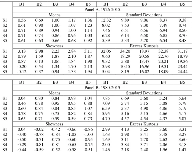
We use 25 portfolios of stocks sorted on market capitalization and the book-to-market ratio to test the conditional CAPM. The portfolios are sourced from the Kenneth R. French data library website. They are obtained from the intersection of five portfolios formed on size (ME, market equity) and five portfolios formed on the book-to-market ratio (BM, book equity-to-market equity). The size breakpoints are the market equity quintiles at the end of June of year t, the BM breakpoints are book-to-market ratio quintiles obtained as book equity as at the fiscal year end t-1 divided by market equity at the same date. Portfolios are held from July of year t to June of year t+1, and they are reformed each year in July. Table 1 provides descriptive statistics for the 25 ME/BM portfolios. Panel A shows the results for the full sample period 1926-2015. The average excess return increases monotonically with the BM ratios ranging from 0.56% for the smallest stocks with the lowest market ratios to 1.36% for the smallest stocks with the highest book-to-market ratios. The monotonic pattern is evident for all of the quintiles. Interestingly, the value portfolios have a higher beta.

Panel B of Table 1 provides descriptive statistics for the 25 ME/BM portfolios for the subsample period 1980-2015. The evidence of a value premium is even more evident here, with returns increasing monotonically with BM ratios for all of the quintiles. The panel shows that standard deviations are negatively correlated with market capitalization, while value portfolios are characterized by negative skewness and larger kurtosis than the other portfolios. Finally, in unreported results, we found that beta tends to be negatively correlated with size and positively correlated with the book-to-market factor.

[Insert Table 1 about here]

5.1. The bull and bear regimes

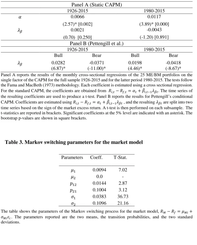
The results of the standard Fama and MacBeth methodology (1973) to test the CAPM are reported in Panel A of Table 2 for the periods 1926-2015 and 1980-2015, respectively. The results strongly contradict the underlying theory. The CAPM is rejected for each period as the risk premium is positive but insignificant for the full sample, and negative though insignificant for the more recent period. The intercept is positive and highly significant,

18

especially for the subsample, a result which is inconsistent with the standard CAPM. Such a positive intercept suggests that some risk factors may have been omitted from the model. However, a positive intercept, though not perhaps of this magnitude, may also be explained by the zero beta rate being different from the risk-free rate. For example, if the true return generating process were

𝑅𝑅𝑖𝑖𝑖𝑖 = 𝛾𝛾𝑧𝑧𝑖𝑖+ 𝛽𝛽𝑚𝑚𝑖𝑖𝑅𝑅𝑚𝑚𝑖𝑖+ 𝛽𝛽𝐹𝐹𝑖𝑖𝐹𝐹𝑖𝑖+ 𝜀𝜀𝑖𝑖𝑖𝑖

where 𝛾𝛾_{𝑧𝑧𝑖𝑖} = 𝑅𝑅_{𝑓𝑓𝑖𝑖}+ 𝛾𝛾_0𝑖𝑖 is the zero beta rate, and 𝐹𝐹_𝑖𝑖 is some pricing factor. Taking expectations gives,

𝐸𝐸(𝑅𝑅𝑖𝑖𝑖𝑖− 𝑅𝑅𝑓𝑓𝑖𝑖) = 𝐸𝐸(𝛾𝛾0𝑖𝑖) + 𝐸𝐸(𝛽𝛽𝐹𝐹𝑖𝑖𝐹𝐹𝑖𝑖) + 𝛽𝛽𝑚𝑚𝑖𝑖𝐸𝐸(𝑅𝑅𝑚𝑚𝑖𝑖)

So ignoring 𝐸𝐸(𝛾𝛾_0𝑖𝑖) or 𝐸𝐸(𝛽𝛽_{𝐹𝐹𝑖𝑖}𝐹𝐹_𝑖𝑖) creates the potential for having a significant intercept in a standard CAPM. Thus, the common empirical problems of the CAPM documented by the vast majority of existing studies are confirmed at this point.

[Insert Table 2 about here]

In Panel B of Table 2, we introduce two regimes, bull and bear, based on the ex-post excess market return of Pettengill et al. (1995). The table confirms asymmetry in the market premiums. The full sample shows a positive return of 2.82% in bull markets and a negative return of -3.71% in bear markets. For the subsample 1980-2015, the returns are 1.98% and -4.18%, respectively.

One limitation of the dual test of Pettengill et al., in which two different risk premiums are estimated conditional on the sign of the excess market return, is that investors do not know, ex-ante, whether the market will be bullish or bearish at any given moment in time. Moreover, a bullish/bearish market might evidence some negative/positive market excess returns, even though it is fundamentally characterised by an overall positive/negative trend. Therefore, to reflect real-world observation, some negative (positive) return periods should actually be accommodated within the bullish (bearish) estimation.

The filtered probabilities of the bull and bear regime, estimated using the Expected Maximization algorithm of Hamilton (1989), are reported in Figure 1. The two regimes are each estimated with a different mean and different standard deviation. When applying the switching regimes methodology, the mean in the bearish market is found not to be

19

significantly different from zero. Specifically, the bear market average return is found to be -1.45% but with a t-statistic of -1.28, which is insignificant at the 5% level. Therefore, the switching regime is repeated, imposing the average return in a bear market to be zero.

[Insert Figure 1 about here]

From Table 3, it can be noted that the bullish regime is the more likely of the two, and is characterized by a positive average market return of 0.94% and a standard deviation of 3.83%. In contrast, the bearish market is characterized by low returns (on average 0%) and a high standard deviation of 10.96%. The bullish regime is typical of the 1940s, 1950s, 1980s, for a prolonged period in the 1990s, and in the recovery following the dotcom crisis in the early years of the new millennium. The bearish regime is typical of the year 1929, the mid-1970s, the early and late 1980s, the high volatility period of the late 1990s, the early years of the new millennium, and of course the financial crisis of 2007. Both regimes are persistent with very small transition probabilities. Indeed, there is a 10.04% transition probability from a bearish regime to a bullish regime, and only a 1.44% transition probability from a bullish regime to a bearish regime.

[Insert Table 3 about here]

The two regimes are quite distinct. The bullish regime has a positive average return and low volatility, whereas the bearish regime has a low average return and high volatility. Contrary to the logic of Pettengill et al. (1995), many realised market returns are positive during a bear market. Our results also suggest that the positive returns actually offset the negative ones. This is consistent with increased volatility during market turmoil.

The bullish and bearish regimes might then be defined more precisely as a bullish quiet regime and a bearish high volatility regime that might lead to swings between high positive and high negative returns. As the risk premium for the market portfolio is a function of both the degree of risk aversion and volatility, the two regimes (while different in terms of volatility and returns) should capture the variation in risk aversion and hence reveal the

20

time-varying risk premium. Thus, while risk aversion is not modelled directly in this paper, it is revealed indirectly by the time-varying risk premium which depends on the regime. Figure 1 shows that the market is located, with high probability, in a bullish regime 87.46% of the time, and in a bearish regime only 12.54% of the time. This observation is important as the different risk premiums demanded in a bull and a bear market may produce a positive weighted average risk premium. In particular, it might be the case that the conditional risk premiums and the time-varying factor sensitivities are correlated in such a way that they explain the main anomalies of the standard CAPM.

5.2. Individual fixed effects panel for the conditional CAPM

We use an individual fixed effects panel data model, such that the intercepts are allowed to vary across individual assets (the 25 ME/BM-sorted portfolios), but are kept constant over time. The intercepts are thus able to capture an individual effect that impacts upon the portfolios but does not change over time. However, one consequence of using fixed effects estimation is that the intercept is removed and therefore only the two risk premiums are obtained. In unreported results, we estimated random effects models as alternatives to the fixed effects models. In each case the random effects model was rejected by the Hausman (1978) specification test.

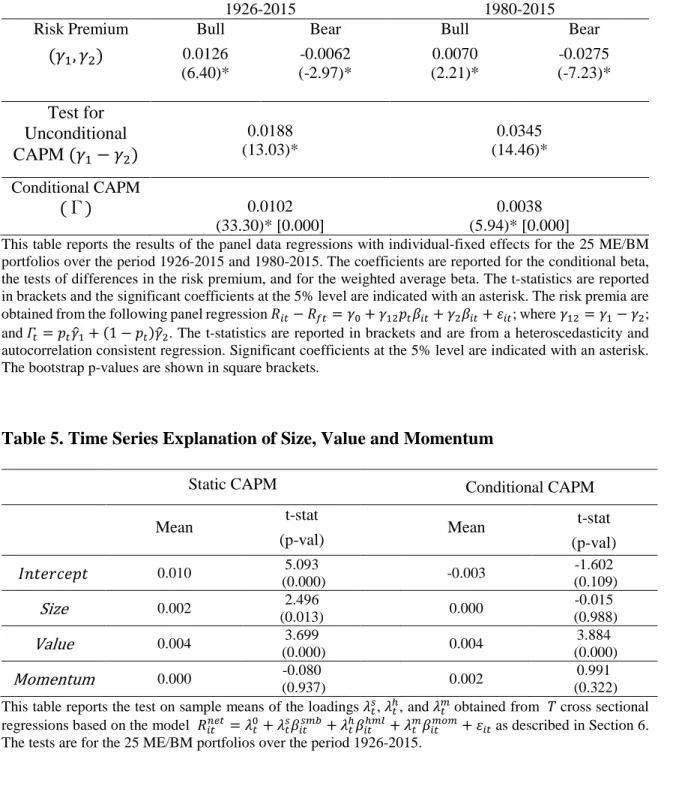
Table 4 reports results on the risk premiums, the unconditional CAPM, and the conditional CAPM. The betas for the unconditional model are obtained from five year rolling window estimates as in Fama and MacBeth (1973). The conditional model is obtained first using a DCC GARCH approach to obtain the betas, and then using a panel model to estimate the risk premiums. We use excess returns in all cases. The results show that for the full sample period, the bear risk premium is significant and negative (-0.62% per month), whereas the bull risk premium is significant and positive (1.26% per month). Therefore, the conditional signs of the risk premiums are both significant and consistent with expectations. The unconditional CAPM is strongly rejected as the difference between the two risk premiums for the full sample is 1.88%, and is statistically significant at the 5% level.

When the time series of the risk premium is tested using an autoregressive model with standard errors corrected for autocorrelation, the results show that the risk premium

21

becomes significantly positive at 1.02% per month for the full sample (and 0.38% for the subsample). Our results therefore support a conditional CAPM in which beta is priced, particularly in bullish markets. This finding is interesting as it potentially provides a partial explanation for the cross-section of returns observed in the most challenging portfolios in the empirical asset pricing literature.

For the more recent sub-period of 1980-2015, which is widely held to be the most challenging to explain, the results show a positive market premium in the bullish market of 0.70%, with a negative risk premium in the bearish market of -2.75% which is clearly of larger magnitude in absolute terms than in a bull market. More interestingly, the weighted average risk premium is positive and significant at 0.38% per month or 4.65% annualised. Thus, the risk premium has declined over the sample period, a phenomenon well documented in the existing literature, though it also confirms that the systematic risk measured by beta is still rewarded by the market, as we expect from theory, even for portfolios sorted on market capitalization and the book to market ratio. The unconditional CAPM is again strongly rejected as the difference between the two risk premiums is 3.45%, and is statistically significant at the 5% level.

[Insert Table 4 about here]

6. Time series and cross section explanation of returns

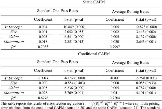
Although the statistical significance of the estimated conditional risk premiums is useful evidence that our conditional model is a non-trivial improvement on the static CAPM, this evidence is nevertheless incomplete and should be complemented by contrasting the cross sectional and time series performance of the conditional model with that of the static model. In this section, we first provide some time series results on the premiums associated with size, value and momentum. We then discuss the pricing errors of the static and conditional models.

If our conditional model explained size, value and momentum, then the loadings from the three factors should not be priced. Thus, we run 𝑇𝑇 cross sectional regressions with the three factors on net returns

22

𝑅𝑅𝑖𝑖𝑖𝑖𝑛𝑛𝑛𝑛𝑖𝑖 = 𝜆𝜆𝑖𝑖0+ 𝜆𝜆𝑖𝑖𝑠𝑠𝛽𝛽𝑖𝑖𝑖𝑖𝑠𝑠𝑚𝑚𝑠𝑠+ 𝜆𝜆𝑖𝑖ℎ𝛽𝛽𝑖𝑖𝑖𝑖ℎ𝑚𝑚𝑚𝑚+ 𝜆𝜆𝑖𝑖𝑚𝑚𝛽𝛽𝑖𝑖𝑖𝑖𝑚𝑚𝑚𝑚𝑚𝑚 + 𝜀𝜀𝑖𝑖𝑖𝑖 (19)

The time series test is then performed on sample means of 𝜆𝜆_𝑖𝑖𝑠𝑠, 𝜆𝜆_𝑖𝑖ℎ, and 𝜆𝜆_𝑖𝑖𝑚𝑚.

The net returns are given by 𝑅𝑅_{𝑖𝑖𝑖𝑖}𝑛𝑛𝑛𝑛𝑖𝑖 = 𝑅𝑅_{𝑖𝑖𝑖𝑖} − 𝑅𝑅_{𝑓𝑓𝑖𝑖} − 𝛾𝛾�₁₂𝑝𝑝_𝑖𝑖𝛽𝛽_{𝑖𝑖𝑖𝑖}− 𝛾𝛾�₂𝛽𝛽_{𝑖𝑖𝑖𝑖} for the conditional CAPM (the conditional betas are obtained from a DCC model). For the static CAPM, the net returns are given by 𝑅𝑅_{𝑖𝑖𝑖𝑖}𝑛𝑛𝑛𝑛𝑖𝑖 = 𝑅𝑅_{𝑖𝑖𝑖𝑖}− 𝑅𝑅_{𝑓𝑓𝑖𝑖} − 𝜆𝜆_𝛽𝛽𝛽𝛽_{𝑖𝑖𝑖𝑖}, where the betas are obtained from a five year rolling window and 𝜆𝜆_𝛽𝛽 is the standard CAPM estimated risk premium.

The loadings, 𝛽𝛽_{𝑖𝑖𝑖𝑖}𝑠𝑠𝑚𝑚𝑠𝑠, 𝛽𝛽_{𝑖𝑖𝑖𝑖}ℎ𝑚𝑚𝑚𝑚 and 𝛽𝛽_{𝑖𝑖𝑖𝑖}𝑚𝑚𝑚𝑚𝑚𝑚 are estimated from time series models using five year rolling windows

𝑅𝑅_{𝑖𝑖𝑖𝑖}𝑛𝑛 _{= 𝛽𝛽}

0+ 𝛽𝛽𝑖𝑖𝑖𝑖𝑚𝑚𝑘𝑘𝑖𝑖𝑅𝑅𝑚𝑚𝑖𝑖𝑛𝑛 + 𝛽𝛽𝑖𝑖𝑖𝑖𝑠𝑠𝑚𝑚𝑠𝑠𝑆𝑆𝑆𝑆𝑆𝑆𝑖𝑖+ 𝛽𝛽𝑖𝑖𝑖𝑖ℎ𝑚𝑚𝑚𝑚𝐻𝐻𝑆𝑆𝐿𝐿𝑖𝑖+ 𝛽𝛽𝑖𝑖𝑖𝑖𝑚𝑚𝑚𝑚𝑚𝑚𝑆𝑆𝑀𝑀𝑆𝑆𝑖𝑖+ 𝜀𝜀𝑖𝑖𝑖𝑖

where 𝑅𝑅𝑛𝑛 indicates excess return. Table 5 provides tests for the (time) average risk premiums for the three factor sensitivities. For the conditional CAPM, only the value premium is significant. Size and momentum appear to be explained by the model. On the other hand, for the static CAPM both size and value remain unexplained.

[Insert Table 5 about here]

For the cross section comparison, we calculate the pricing errors from the two models as follows:

𝜖𝜖𝑖𝑖𝐶𝐶𝑚𝑚𝑛𝑛𝐶𝐶 = 𝐸𝐸(𝑅𝑅𝑖𝑖𝑖𝑖− 𝑅𝑅𝑓𝑓𝑖𝑖) − 𝐸𝐸(𝛤𝛤𝑖𝑖)𝐸𝐸(𝛽𝛽𝑖𝑖𝑖𝑖) − 𝐶𝐶𝐶𝐶𝐶𝐶(𝛤𝛤𝑖𝑖, 𝛽𝛽𝑖𝑖𝑖𝑖) (20)

𝜖𝜖𝑖𝑖𝑆𝑆𝑖𝑖𝑎𝑎𝑖𝑖 = 𝐸𝐸(𝑅𝑅𝑖𝑖𝑖𝑖− 𝑅𝑅𝑓𝑓𝑖𝑖) − 𝜆𝜆𝛽𝛽𝐸𝐸(𝛽𝛽𝑖𝑖𝑖𝑖) (21)

where, as before, the conditional betas are from a DCC model, the standard CAPM betas are from five year rolling univariate regressions, and 𝜆𝜆_𝛽𝛽 is the standard CAPM estimated risk premium. The pricing error from the static CAPM is more than double that of the conditional CAPM. The average absolute error is 0.28% for the conditional model, against 0.65% for the static model.

23

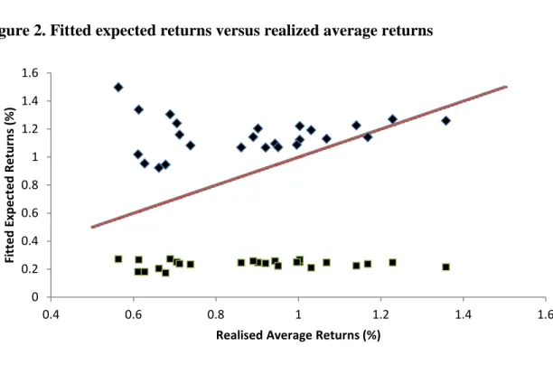
Another way of looking at the pricing error is by visually comparing the performance of the two models. In Figure 2, we plot the fitted expected returns from the two models against the realised average return. A perfect fit requires fitted returns to lie on the 45-degree line through the origin. Clearly, neither model is anywhere near a perfect fit. However, the conditional fit improves on two fronts. First, in terms of level, the static CAPM under-estimates average realised returns, which explains why the intercept in the estimated model is positive and highly significant. More importantly, the relationship between fitted and observed returns is almost perfectly flat, due mainly to a small and insignificant risk premium. Note that the static CAPM risk premium for the later period (1980-2015) is negative, so the fit is even worse for that period. On the other hand, the scale of the conditional fit is closer to that of the realised average returns. Apart from four outliers (top left of Figure 2), the relationship is steeper relative to the static CAPM. These outliers are all at the bottom BM (growth) stocks. This is in line with our earlier finding that the conditional model fails to explain the value anomaly. Moreover, most predicted returns are over-stated. This is possibly due to either an excessively high risk premium and/or low variability in the beta estimates which flattens the relationship between fitted and realised average returns.

[Insert Figure 2 about here]

Finally, we regress both sets of pricing errors on the size, value and momentum sensitivities. We use two types of estimates. The first was standard multivariate betas, obtained from a single time series for each portfolio 𝑖𝑖 = 1, … , 𝑁𝑁

𝑅𝑅𝑖𝑖𝑖𝑖𝑛𝑛 = 𝛽𝛽0+ 𝛽𝛽𝑖𝑖𝑚𝑚𝑘𝑘𝑖𝑖𝑅𝑅𝑚𝑚𝑖𝑖𝑛𝑛 + 𝛽𝛽𝑖𝑖𝑠𝑠𝑚𝑚𝑠𝑠𝑆𝑆𝑆𝑆𝑆𝑆𝑖𝑖+ 𝛽𝛽𝑖𝑖ℎ𝑚𝑚𝑚𝑚𝐻𝐻𝑆𝑆𝐿𝐿𝑖𝑖+ 𝛽𝛽𝑖𝑖𝑚𝑚𝑚𝑚𝑚𝑚𝑆𝑆𝑀𝑀𝑆𝑆𝑖𝑖+ 𝜀𝜀𝑖𝑖𝑖𝑖 (22)

The second set of sensitivities is obtained from five year rolling regressions for each portfolio, and averaging sensitivities. That is, for each portfolio 𝑖𝑖 = 1, … , 𝑁𝑁, we perform T regressions

24

The cross section of sensitivities, (𝛽𝛽̅_𝑖𝑖𝑠𝑠𝑚𝑚𝑠𝑠, 𝛽𝛽̅_𝑖𝑖ℎ𝑚𝑚𝑚𝑚, 𝛽𝛽�_𝑖𝑖𝑚𝑚𝑚𝑚𝑚𝑚), are obtained by averaging across time. Table 6 presents the cross section regression results of pricing errors on the factor sensitivities. There is little difference between the multivariate and rolling betas, except that the rolling betas are slightly more correlated with the pricing errors as can be seen by the coefficient of determination. Regardless of the sensitivity estimates, the conditional CAPM clearly explains away the size effect as the slope associated with the size beta is highly insignificant. The static CAPM, on the other hand, does not explain size. Both models, however, fail to explain value and momentum effects in the cross section.

[Insert Table 6 about here]

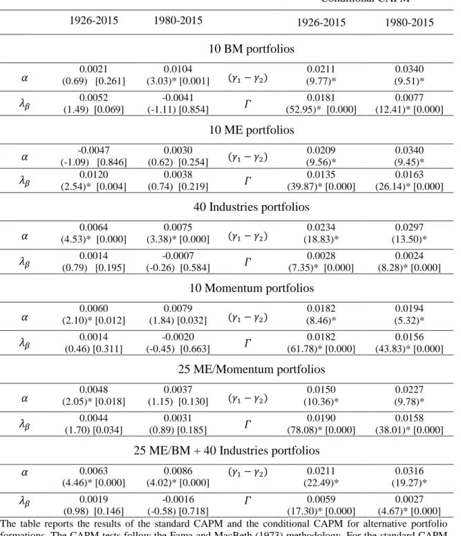
6. Robustness check

In order to check the robustness of our conditional approach, the empirical test is conducted on a set of different portfolios obtained from the website of Kenneth R. French, that of 10 ME, 10 BM, 10 Momentum, 25 ME/Momentum, 10 Beta, 40 industries, and the 65 combined ME/BM and industry portfolios. The results, reported in Table 7, confirm that the Fama and MacBeth test leads to a firm rejection of the unconditional CAPM (only the full sample, 10 ME portfolios, show a significant estimated risk premium). In other words, the unconditional CAPM produces no evidence of a positive risk premium. The conditional CAPM produces positive and significant risk premiums for all choices of portfolios. However, the scale of the premium appears to depend on the number of portfolios, varying between 1.3% and 1.9% for 25 or less portfolios, but dropping to 0.2% for the 40 industries portfolios and 0.6% for the 65 ME/BM and industries portfolios.

Overall, our version of the conditional CAPM consistently rejects the static CAPM, and finds positive risk premiums for all portfolio groups. But, it does not seem to be robust to the choice of test portfolios, with larger sets producing lower risk premiums. The results, however, seem to be robust to the choice of the sample period. The sign and significance of the risk premiums are unchanged for the sub-sample (1980-2015), and the scale of the premiums is similar except for the 10 BM portfolios.

25 7. Conclusion

This paper investigates the performance of a conditional CAPM using both conditional time-varying risk sensitivities and conditional time-varying risk premiums. Conditional market betas are estimated using a DCC GARCH approach. The conditional risk premiums are estimated by first identifying the probability of a bull and a bear regime according to a Markov Switching process, and then estimating the conditional risk premiums using a panel regression.

Our main empirical findings are several fold. First, the unconditional model is always rejected in favour of a conditional model incorporating time-varying beta and risk premiums. Second, although the conditional model is supported for the full as well as the sub-sample, the implied unconditional risk premiums appear to have changed substantially in the recent period. The conditional CAPM suggests a risk premium of 1.02% for the full sample, but this drops to 0.38% per month for the period 1980-2015. Moreover, the results are not robust across alternative test assets. The risk premium is significant but particularly low for the industry portfolios. Third, despite statistical significance, our conditional model fails to explain the value and momentum anomalies. However, conditioning appears to explain the size anomaly.

Our results suggest that while beta risk is priced unconditionally, estimating and testing the unconditional risk premium is only possible through the use of conditional models. Using both time-varying betas and time-varying risk premiums is logical as well as empirically sound.

Although we do not model time-varying risk aversion directly, risk aversion is accounted for indirectly through the consideration of two market regimes in which investors tolerate negative realised premiums during bear markets in exchange for positive premiums during bull markets. Thus, unconditionally risk averse investors may appear to be conditionally risk seekers during downturns by accepting negative returns. But they only do this in the knowledge that, in probability, the upmarket will compensate them for bearing the bear market losses.

The bull and bear regimes are only known with a probability, which we estimate using a Markov Switching process. This enables us to avoid exogenous identification of the regime by, for example, using the sign of the monthly market return.

26

Our simple conditional model provides evidence that beta is positively rewarded by the market. Unconditional models are unable to provide such evidence, not because beta is irrelevant, but simply because the unconditional version of the CAPM employed in previous tests is misspecified. Nevertheless, although the conditional CAPM is a clear improvement on the static CAPM, we cannot claim that it is a definitive answer to the three or four factor model. The small growth portfolios remain largely unexplained by our conditional beta despite the high estimated price of risk. However, this limitation is not unique to the conditional CAPM. The Fama and French (1996: 57) three factor model also leaves “… a large negative unexplained return for the portfolio of stocks in the smallest size and lowest BE/ME quintiles.” Their model also fails to explain the continuation of short-term returns, and was in any case rejected by the Gibbons, Ross and Shanken (1989) test.

Our paper has four main limitations. First, we use a three-pass approach. In the first two passes, the market state probabilities and the conditional betas are estimated, respectively. These estimates are then used in the third pass to estimate the risk premiums. There is a clear risk that the errors-in-variables problem has affected our conclusions. Although the errors-in-variables problem is usually less important when portfolios are used as test assets, we have tried to mitigate this problem partially by using the wild bootstrap to calculate p-values. Nevertheless, future work should consider estimating both sets of parameters simultaneously in a multivariate conditional model. However, this is no simple task because of the curse of dimensionality. Second, our conditional betas appear to be flat. We have relied on the dynamic conditional model of Engle (2002) to estimate conditional betas, but future work should consider possibly simpler alternatives such as those employed by Lewellen and Nagel (2006). Third, in contrast to the unconditional CAPM, the pricing error is not expected to be zero. The conditional CAPM implies an additional term, namely the covariance between beta and the risk premium. Future work should therefore focus on testing the additional hypothesis that the pricing error is equal to the beta-risk premium covariance. It should be noted, though, that this is not a straightforward task as it involves testing the equality of two cross sectional series of unobserved variables. Last, and most important, the Fama and French three factors model remains hard to beat, and the 25 ME/BM portfolios hard to explain. We have specifically chosen these portfolios because

27

they are hard to explain. However, both our model and the three factor model fail to explain growth portfolios. This leaves the potential for a conditional three or four factor model in which the conditional expected return (ex-post risk premium) depends on the probabilities of bull and bear markets.

A different direction would be to extend a multi-moments asset pricing model such as Vendrame et al. (2016). In that paper, the size premium could not be explained away. Conditioning on the bull and bear market could improve a multi-moments explanation of average returns.

28 References

Adrian, T., and Franzoni, F. (2009) Learning about beta: time varying factor loadings, expected returns, and the conditional CAPM. Journal of Empirical Finance. 16, pp. 537-556.

Andersen, T., Bollerslev, T., Diebold, F., and Labys, P. (2003) Modeling and forecasting realized volatility. Econometrica. 71, pp. 529-626.

Ang, A., and Chen, J. (2007) CAPM over the long run: 1926-2001. Journal of Empirical

Finance. 14, pp. 1-40.

Avramov, C., and Chordia, T. (2005) Asset pricing models and financial market anomalies.

Review of Financial Studies. 19, pp. 1001-1040.

Bali, T. and Engle, R. (2010) Resurrecting the conditional CAPM with dynamic conditional correlations. Working Paper. New York University Stern School of Business. Banz, R. (1981) The relationship between return and market value of common stocks.

Journal of Financial Economics. 9, pp. 3-18.

Basu, S. (1977) Investment performance of common stocks in relation to their price-earnings ratios: A test of the Efficient Market Hypothesis. Journal of Finance. 32, pp. 663-682.

Bauer, R., Cosemans, M., and Schotman, P. (2010) Conditional asset pricing and stock market anomalies in Europe. European Financial Management. 16, pp. 165-190.

Bhandari, L. (1988) Debt/equity ratio and expected common stock returns: Empirical evidence. Journal of Finance. 43, pp. 507-528.

Black, F., Jensen, M., and Scholes, M. (1972) The Capital Asset Pricing Model: Some empirical tests. Studies in the Theory of Capital Markets. Ed. New York: Praeger Publishers.

Blume, M., and Friend, I. (1973) A new look at the capital asset pricing model. Journal of

Finance, 28, pp. 19-34.

Bodurtha, J., and Nelson, M. (1991) Testing the CAPM with time-varying risks and returns.

Journal of Finance. 46, pp. 1485-1505.

Bollerslev, T., Engle, R., and Wooldridge, J. (1988) A Capital Asset Pricing Model with time varying covariances. Journal of Political Economy. 96, pp. 116-131.

29

Brown, S., Goetzmann, W., and Ross, S. (1995) Survival. Journal of Finance, 50, pp. 853-873.

Campbell, J., and Shiller, R. (1988) The dividend-price ratio and expectations of future dividends and discount factors. Review of Financial Studies. 1, pp. 195-227.

Carhart, M. (1997) On persistence in mutual fund performance. Journal of Finance. 52, pp. 57-82.

Cochrane, J. (2001) Asset Pricing. Princeton University Press.

Cox, J., Ingersoll Jr, J., and Ross, S. (1985) An intertemporal general equilibrium model of asset prices. Econometrica. 53, pp. 363-384.

Davidson, J., A. Monticini and Peel, D. (2007) Implementing the Wild Bootstrap using a two-point distribution, Economics Letters. 96, pp. 309-315.

Dittmar, R. (2002) Nonlinear pricing kernels, kurtosis preference and cross-section of equity returns. Journal of Finance. 57, pp. 369-403.

Douglas, G. (1969) Risk in the equity markets: An empirical appraisal of market efficiency.

Yale Economic Essays. 9, pp. 3-45.

Durbin, J., and Koopman, S.J. (2001). Time Series Analysis by State Space Methods. Oxford University Press. Oxford.

Engle, R. (2002) Dynamic conditional correlation - A simple class of multivariate GARCH models. Journal of Business and Economic Statistics. 20, pp. 339-350.

Fama, E., and French, K. (1988) Dividend yields and expected stock returns. Journal of

Financial Economics. 22, pp. 3-25.

Fama, E., and French, K. (1992) The cross-section of expected stock returns. Journal of

Finance. 47, pp. 427-465.

Fama, E., and French, K. (1993) Common risk factors in the returns on stocks and bonds.

Journal of Financial Economics. 33, pp. 3-56.

Fama, E., and French, K. (1996) Multifactor explanations of asset pricing anomalies.

Journal of Finance. 51, pp. 55-84.

Fama, E., and MacBeth, J. (1973) Risk, return and equilibrium: Some empirical tests.

Journal of Political Economy. 81, pp. 607-636.

Ferson, W., and Harvey, C. (1991) The variation of economic risk premiums. Journal of

30

Ferson, W., and Harvey, C. (1999) Conditioning variables and the cross section of stock returns. Journal of Finance. 54, pp. 1325-1360.

Freeman, M., and Guermat, C. (2006) The conditional relationship between beta and returns: a reassessment. Journal of Business Finance and Accounting. 33, pp. 1213-1239. Hamilton, J. (1989) A new approach to the economic analysis of nonstationary time series and the business cycle. Econometrica. 57, pp. 357-384.

Gibbons, M., Ross, S., and Shanken, J. (1989) A test of the efficiency of a given portfolio.

Econometrica. 57, pp. 1121-1152.

Hamilton, J. (1994) Time Series Analysis. Princeton

Hansen, B. (2000) Sample splitting and threshold estimation. Econometrica, 68, pp. 575-603.

Hansen, L., and Jagannathan, R. (1997) Assessing specification errors in stochastic discount factor models. Journal of Finance. 52, pp. 557-590.

Hausman, J. (1978) Specification tests in econometrics. Econometrica. 46, pp. 1251– 1271.

Jagannathan, R., and Wang, Z. (1996) The conditional CAPM and the cross-section of expected returns. Journal of Finance. 51, pp. 3-54.

Jagannathan, R., and Wang, Z. (1998) An asymptotic theory for estimating beta-pricing models using cross-sectional regression. Journal of Finance. 53, pp. 1285-1309.

Jorion, P., and Goetzmann, W. (1999) Global stock markets in the twentieth century.

Journal of Finance. 54, pp. 953-980.

Jostova, G., and A. Philipov, A. (2005) Bayesian analysis of stochastic betas. Journal of

Financial and Quantitative Analysis. 40, pp. 747-778.

Kan, R., Robotti, C., and Shanken, J. (2013) Pricing model performance and the two-pass cross-sectional regression methodology. Journal of Finance. 68, pp. 2617-2649.

Lambert, M., and Hubner, G. (2013) Comoment risk and stock returns. Journal of

Empirical Finance. 23, pp. 191-205.

Lettau, M., and Ludvigson, S. (2001) Resurrecting the (C)CAPM: A cross-sectional test when risk premia are time-varying. Journal of Political Economy. 109, pp. 1238-1287. Lewellen, J., and Nagel, S. (2006) The conditional CAPM does not explain asset-pricing anomalies. Journal of Financial Economics. 82, pp. 289-314.