c
EFFICIENT VISUALIZATION FOR LARGE-SCALE AND HIGH-DIMENSIONAL SINGLE-CELL DATA
BY JUHO KIM
THESIS
Submitted in partial fulfillment of the requirements
for the degree of Master of Science in Electrical and Computer Engineering in the Graduate College of the
University of Illinois at Urbana-Champaign, 2017
Urbana, Illinois Advisers:
Assistant Professor Oluwasanmi Koyejo Assistant Professor Jian Peng
ABSTRACT
This thesis is concerned with developing an efficient and scalable visualiza-tion method for large-scale and high-dimensional single-cell data. Single-cell analysis can uncover the mysteries in the state of individual cells and en-able us to construct new models of heterogeneous tissues. State-of-the-art technologies for single-cell analysis have been developed to measure the prop-erties of single cells and detect hidden information. They are able to provide the measurements of dozens of features simultaneously in each cell. However, due to the high-dimensionality, heterogeneous complexity and sheer enormity of single-cell data, its interpretation is challenging. Thus, new methods to overcome high-dimensionality are necessary. Here, we present a computa-tional tool that allows efficient visualization of high-dimensional single-cell data onto a low-dimensional (2D or 3D) space while preserving the similarity structure between single cells. We first construct a network that can rep-resent the similarity structure between the high-dimensional reprep-resentations of single cells, and then embed this network into a low-dimensional space through an efficient online optimization method based on the idea of neg-ative sampling. Using this approach, we can preserve the high-dimensional structure of single-cell data in an embedded low-dimensional space that fa-cilitates visual analyses of the data.
ACKNOWLEDGMENTS
First and foremost, I would like to thank my advisers, Professor Jian Peng and Professor Oluwasanmi Koyejo, for their patient support and guidance throughout my graduate study and research process. They always helped and encouraged me to find the right research directions and gave me invaluable technical advice to improve my understanding of research. I also thank my friends in the Machine Learning and Computational Biology Research Group for their valuable discussions and suggestions. Lastly, I sincerely thank my wife Hyunji and my parents for their love and patience.
TABLE OF CONTENTS
LIST OF TABLES . . . vi
LIST OF FIGURES . . . vii
LIST OF ABBREVIATIONS . . . viii
CHAPTER 1 INTRODUCTION . . . 1
1.1 Single-cell Analysis . . . 1
1.2 Single-cell Technologies . . . 2
1.3 Motivation and Related Work . . . 2
1.4 Main Contributions . . . 4
1.5 Thesis Organization . . . 5
CHAPTER 2 METHODS . . . 6
2.1 Outline of Proposed Method . . . 6
2.2 Notation . . . 7
2.3 Construction ofk-nearest Neighbor Network . . . 7
2.4 Network Embedding into a Low-dimensional Space . . . 9
2.5 Algorithms and Implementation . . . 11
CHAPTER 3 EXPERIMENTS . . . 12
3.1 Data and Data Preprocessing . . . 12
3.2 Baselines . . . 13 3.3 Experimental Setting . . . 13 CHAPTER 4 RESULTS . . . 15 4.1 Visualization . . . 15 4.2 Computation Time . . . 17 4.3 Clustering . . . 20
CHAPTER 5 WEB-BASED INTERACTIVE VISUALIZATION . . . 24
CHAPTER 6 CONCLUSION . . . 26
LIST OF TABLES
3.1 Parameters for constructing k-NN networks. . . 14 3.2 Parameters for embedding the constructed k-NN networks. . . 14
LIST OF FIGURES
1.1 Single-cell analysis can help us understand cellular-level
heterogeneity and cell subpopulation expression profiles. . . . 1 1.2 Single-cell RNA sequencing workflow. Source from Wikipedia
(https://goo.gl/AYBEXF) . . . 3 2.1 Outline of visualization of large-scale and high-dimensional
single-cell data. (1) Construction of a k-nearest neighbor
network and (2) embedding the network into a 2D space. . . . 6 4.1 Visualization of our method for the data set which contains
mice bone marrow replicate 7. . . 16 4.2 Visualization of viSNE for the data set which contains mice
bone marrow replicate 7. . . 17 4.3 Comparison of the computation time of viSNE and our
method with respect to the number of single-cell data samples. 18 4.4 Separate analysis of the computation time for
construct-ing a k-NN network and for embedding the network with
regard to the number of single-cell data samples. . . 19 4.5 Effectiveness of the multiple threads for speedup of our method. 20 4.6 Comparison of the clustering performance of viSNE and
our method when using two-dimensional vectors with
re-spect to the number of clusters. . . 22 4.7 Comparison of the clustering performance of viSNE and
our method when using two-dimensional vectors with
re-spect to the number of clusters. . . 23 5.1 Compare different visualization methods and reproduce
vi-sualization results based on our web-based tool. . . 24 5.2 Our web-based system can compare the results from
LIST OF ABBREVIATIONS
ASGD Asynchronous Stochastic Gradient Descent CLP Common Lymphoid Progenitor
CMP Common Myeloid Progenitors GMP Granulocyte Monocyte Progenitors HSC Hematopoietic Stem Cell
k-NN k-Nearest Neighbor
MEP Megakaryocyte Erythroid Progenitors MPP Multi-Potent Progenitors
NCE Noise-Contrastive Estimation
NK Natural Killer
NKT Natural Killer T
PCA Principle Component Analysis scRNA-seq Single-Cell RNA Sequencing SGD Stochastic Gradient Descent
CHAPTER 1
INTRODUCTION
1.1
Single-cell Analysis
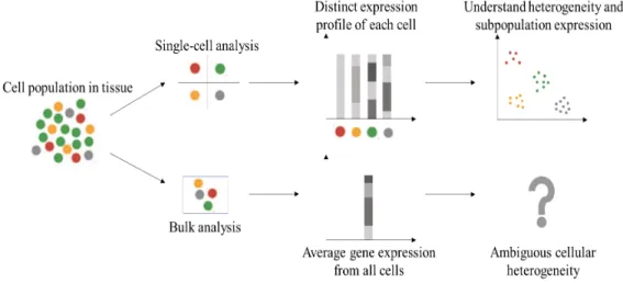
Traditionally, many biological experiments have been conducted on bulk-cell populations [1] with an assumption that cells in the same group share homo-geneous properties. However, some evidence [1–3] shows that heterogeneity can exist even within a small group of cells. The assumption based on homo-geneity of each cell group can distort averages and does not properly explain small but critical changes in individual cells. Each cell can have different biological properties such as cell size, gene expression level, RNA transcript, and bio-marker expression. These variations can be very important to answer previously unsolved questions in stem cell research, cancer biology, and im-munology. As shown in Figure 1.1, single-cell data analysis has contributed to understanding the various and important behaviors of individual cells [1–19].
Figure 1.1: Single-cell analysis can help us understand cellular-level heterogeneity and cell subpopulation expression profiles.
1.2
Single-cell Technologies
The recent development of single-cell technologies has made the analysis more reliable and reasonable. Cytometry is a cutting-edge technology that is used to analyze the optical characteristics of cells. It uses specifically fluorescent light to measure specific antigen using antibodies and DNA or RNA using nu-cleic acid-specific probes. Through these measurements, cytometry can find various cellular features and behaviors including cell size, cell morphology (structure and shape), DNA content, cell count and so on.
As a specific example, mass cytometry [4, 20] is a mass spectrometry that is based on inductively coupled plasma mass spectrometry. In this technique, isotopically pure elements are conjugated with antibodies, which are used for annotating cellular proteins. The nebulized cells are sent to argon plasma. In this process, the conjugated antibodies are ionized. Then, a mass spec-trometer analyzes the metal signals. The signals are detected and recorded as mass cytometry data having a specific format called FCS. Using this mass cytometry, we can measure up to 60 parameters at the same time for tens of thousands of individual cells.
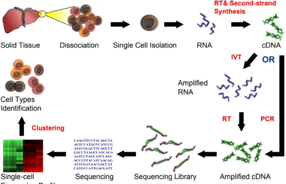
Another widely used single-cell technology is single-cell RNA sequencing (scRNA-seq) [21, 22]. This technique shown in Figure 1.2 is based on next generation sequencing technologies, and it provides the sequence informa-tion for individual cells including the funcinforma-tion of each cell in the micro-environment and high-resolution of cellar-level differences. Specifically, scRNA-seq quantifies the expression profile of each cell. By detecting rare cell types through clustering analyses, this technology can reveal the properties of the subpopulation structure from cell population heterogeneity. Interestingly, by detecting less-frequently discovered cells, scRNA-seq can find the copy-number distribution of the mRNA population. Using this technology, we can capture hundreds or thousands of parameters per cell.
1.3
Motivation and Related Work
Even though the advanced single-cell technologies can provide quality data, such data sets are still difficult to analyze. Traditionally, single-cell data are analyzed in a biaxial scatter plot for two variables at once [23]. However,
Figure 1.2: Single-cell RNA sequencing workflow. Source from Wikipedia (https://goo.gl/AYBEXF)
this method requires the order of dimension squared to represent all pairwise relationships between variables, which is computationally expensive. In ad-dition, scatter plots cannot capture multivariate relationships between more than two variables. Thus, new computational methods have been developed for analyzing single-cell data. For instance, SPADE [6] tries to find hierar-chies of high-dimensional single-cell data showing cellular heterogeneity by clustering of down-sampled cytometry data, constructing minimum span-ning trees, and up-sampling. However, this method considers not each cell itself but cell groups and their behaviors on average. X-shift [12] is recently developed to discover cell subsets and visualize them based on a weighted k-nearest neighbor density estimation.
Another approach to deal with the high-dimensionality of single-cell data is to use dimensionality reduction techniques. Some researchers applied prin-ciple component analysis (PCA) [24] to find low-dimensional projections of single-cell data [25, 26]. Although PCA is possibly the most popular method of dimensionality reduction, it is a linear projection method. Thus, it cannot capture nonlinear structures in single-cell data. In order to address this issue, advanced methods based on nonlinear dimensionality reduction have been
developed. Both viSNE [8] and ACCENSE [10] are based on an algorithm called t-Distributed Stochastic Neighbor Embedding (t-SNE) [27]. viSNE applies t-SNE to mass cytometry data and reveals biologically meaningful relationships from bone marrow and leukemia data. ACCENSE combines the results of t-SNE with kernel-based density estimation and finds subpop-ulations of given single-cell data sets. However, the runtime complexity of t-SNE is O(n2), and that of its accelerated version, Barnes-Hut-SNE [28], is O(nlogn) where n is the number of cells. Thus, both methods require ex-cessive computational time for large-scale single-cell data sets with hundreds of thousands or millions of cells.
Our method is proposed in order to mitigate the computational issue that is raised in the current state-of-the-art methods. We aim to efficiently deal with large-scale single-cell data and to accurately find heterogeneous sub-populations from single-cell data sets that contain many of different types of single cells.
1.4
Main Contributions
In this paper, we propose a scalable embedding-based visualization method for large-scale and high-dimensional single-cell data based on a new graph embedding algorithm, LargeVis [29]. The proposed method constructs a k-nearest neighbor (k-NN) network to find the structure of similarities be-tween high-dimensional single-cell data. This process is accelerated by an ap-proximate k-NN construction method based on random projection trees [30] and neighbor exploring [31]. And then, this approach embeds the high-dimensional single-cell data into a low-high-dimensional space (2D or 3D) while preserving the intrinsic structures between single-cell data points. To do this, we formulate an optimization problem. The utility function of the optimiza-tion is based on the idea from word2vec [32] and negative sampling [32]. The optimization is solved by distributed and parallel computation [33], so it can be easily scaled. The overall runtime complexity of our method is linear with regard to the number of cells, which is much faster than previous single-cell visualization tools such as viSNE [8] and ACCENSE [10]. Also, we show that the quality of our embedding is better in the context of cell subpopulation clustering compared to the embedding quality of viSNE.
1.5
Thesis Organization
This thesis is organized as follows. In Chapter 2, we introduce our proposed method and its algorithmic details. In Chapter 3, we explain the experimen-tal details such as what kinds of single-cell data we used, how to preprocess the data, and our implementation settings. In Chapter 4, we show the re-sults of visualization and compare the quality of our embedding methods with previous state-of-the-art approaches. In Chapter 5, our web-based in-teractive visualization system is introduced with some screen shot images. We conclude this thesis in Chapter 6.
CHAPTER 2
METHODS
2.1
Outline of Proposed Method
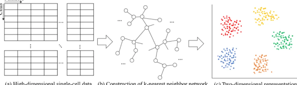
We propose a new approach for visualizing high-dimensional single-cell data via efficient dimensionality reduction based on LargeVis [29]. As shown in Figure 2.1, the algorithm consists of two steps: constructing an approxi-matek-NN network to find the similarity structure between high-dimensional single-cell data, and embedding the constructed network into a 2D or 3D space while preserving the high-dimensional structure in an easily visualized low-dimensional space. Pairwise similarity between single-cell data points is determined by the distance between them in their marker expression rep-resentation space. The core assumption is that numerical proximity in the marker space is proportional to cell similarity.
Figure 2.1: Outline of visualization of large-scale and high-dimensional single-cell data. (1) Construction of a k-nearest neighbor network and (2) embedding the network into a 2D space.
2.2
Notation
We denote a set of high-dimensional single-cell data as X = {xi | xi ∈ Rp, i ∈ [n], p > 3} where p is the dimension of measurements and n is the number of cells in the data; and the embedded representations of cells are denoted as Y ={yi |yi ∈R2orR3, i∈[n]} in a low-dimensional space.
2.3
Construction of
k
-nearest Neighbor Network
Constructing a k-nearest neighbor (k-NN) network is a very crucial step in many applications of machine learning such as a distance-based similarity search, manifold learning, and topological data analysis. Finding the exact k-NN network for large-scale single-cell data is time-consuming because it requires O(n2) time complexity to compute all pairwise distances between all cells in the data set. Approximate methods for constructing a k-NN network have been developed, all of which have a tradeoff between speed and accuracy. Common approaches include locality sensitivity hashing [34], neighbor exploring methods [31], and partitioning methods based on random projection trees [30], k-d trees [35] and k-means trees [35].
As suggested by LargeVis [29], we develop a fast method to construct an approximate k-NN network. We first partition the whole high-dimensional space into two subspaces and generate a tree having only a root node. A set of single cells in each partitioned subspace belongs to child nodes of the root node. Then, for the two subspaces that each set of single cells in the child nodes belongs to, we partition each subspace into two sub-subspaces and generate two child nodes for each child node of the root node. The single cells in each sub-subspace are assigned to each generated child node’s child node. By continuing to partition the space iteratively, we can build a tree that assigns a group of single cells belonging to partitioned small subspaces to its nodes. When the number of cells in a certain node is equal to or less than a predefined threshold, we stop the iterations. The single cells in each leaf node are considered to be candidates of approximate nearest neighbors. The generated tree is called a random projection tree.
By generating many random projection trees, we can increase the accuracy of the construction of a k-NN network, but it is time-consuming. Instead of
building many random projection trees, we use a neighbor search method in order to enhance both the accuracy and the efficiency. Specifically, we search the neighbor j of the neighbor of each node i assuming that its neighbor’s neighbor is likely to be its neighbor also [36]. If the number of neighbors of node i is less than k, the method pushes some searched neighbor’s neighbor j into the set of nearest neighbors of the node i. By iterating this proce-dure, we can improve the accuracy of the construction and finally find our approximate k-NN network. Regarding the accuracy of the k-NN network construction, people can refer to the paper of LargeVis [29], which dealt with several benchmark tests for the accuracy that is influenced by the accuracy of the k-NN construction. The construction process has linear time complexity because we build only a few random projection trees and because searching a certain node’s neighbor’s neighbor requires just a few iterations.
We then calculate the weight of each pairwise edge that represents the similarity structure of the constructed network by the Gaussian kernel, which was also used by t-SNE [27, 28]. The conditional probability that the edge from data xi toxj is observed is first computed by:
pj|i =
exp(−kxi−xjk2/2σi2)
P
(i,k)∈Eexp(−kxi−xkk2/2σi2) pi|i = 0,
(2.1)
where the parameterσi is determined by setting the perplexity, andE is the set of all edges in the k-NN network. To make the network symmetric, the weights are defined as:
wij =
pj|i+pi|j
2n , (2.2)
where n is the number of input data. Since the number kn is much smaller than the number of all pairs (n2), the constructed k-NN network is sparse.
The sparsity of thek-NN network can make us computewij within linear time complexity. Through the steps, our method can find the similarity structure of high-dimensional single-cell data within linear time complexity O(kn).
2.4
Network Embedding into a Low-dimensional Space
Embedding the constructed k-NN network is intended to preserve local and global network topology such that neighbors in the network are near each other in a low-dimensional space. First, for two nodesviandvj, LargeVis [29] defines the probability that they come from the same neighborhood, i.e. the probability that we can observe the edge between two nodes in the k-NN network as:
p(eij = 1 |yi, yj) = f(dist(yi, yj)), (2.3) where f is a transformation function to map the distance between yi and yj into a probability value.
The functionf satisfies the idea that when the distance between two low-dimensional points is small, the probability observing the connection between them is high. After considering some candidates like a multinomial logistic model and a sigmoid function, we chose f(x) = 1+1αx2 where α > 0 due
to its computationally simplicity. The selected function f does not require any normalization across the data set, thus only O(n) runtime is needed for objective evaluation and gradient calculation in the embedding optimization (see below). In addition, we can control the thickness of the tail of the function f by controlling α. When α becomes smaller, its tail gets thicker. When α= 1, f is Student’s t-distribution with degree of freedom one except a scaling factor 1/π.
On the other hand, t-SNE [27] uses the Gaussian kernel pij of Equation (2.1) and a t-distributed kernel qij =
(1+kyi−yjk2)−1
P
i6=k(1+kyi−ykk2)−1 to measure its
high-dimensional and low-high-dimensional similarity, respectively. By minimizing the Kullback-Leibler divergence between two similarities through gradient de-scent, t-SNE finds its low-dimensional embedding. The gradient of its cost function contains the normalization term ofqij. Computing the term requires O(n2). To avoid inefficiency, accelerated t-SNE [28] uses the Barnes-Hut
al-gorithm [37] and reduces its time complexity from O(n2) to O(nlogn). Two
versions of t-SNE are more expensive than our approach.
Like LargeVis [29], we chose Euclidean distance as a distance metric in a low-dimensional space because computing Euclidean distance between em-bedded single-cell data is simple. In addition, we can map each calculated distance to one of the various probability function values since the range of
Euclidean distance is [0,∞).
To embed our high-dimensional data, we define a log likelihood utility function in Equation (2.4) that considers both the probabilities of all edge connections E of the constructed k-NN network and the probabilities of all negative edges EC. Negative edges mean that pairwise single-cell connec-tions are not observed in the k-NN network. This idea originally comes from noise-contrastive estimation (NCE) [38], which considers estimation that dif-ferentiates its observed data from noise using nonlinear logistic regression. Using the idea of NCE, we want to discriminate the same types of cells from different types of cells. Specifically, by maximizing the first term of Equation (2.4), we can make similar single-cells become closer to each other in a low-dimensional space, and by maximizing the second part of Equation (2.4), we can make dissimilar single-cells move away from each other.
J = X
(i,j)∈E
wijlogp(eij = 1|yi, yj) +
X
(i,j)∈EC
γlog(1−p(eij = 1|yi, yj)) (2.4)
However, considering all negative edges is computationally expensive or even intractable when input data are very large. Thus, instead of using all negative edges, we use the idea of negative sampling [32]. This approach considers only a few samples drawn from a noise distribution. We assumed Pn(j)∼d
3/4
j as the noisy distribution wheredj is the degree of nodej, which was used in word2vec [32]. By lettingM be the number of negative samples, we can redefine the utility function as follows:
J = X
(i,j)∈E
wijlogp(eij = 1|yi, yj) + M
X
k=1
Ejk∼Pn(j)γlog(1−p(eijk = 1|yi, yjk))
(2.5) Then, we optimized Equation (2.5) by applying asynchronous stochastic gradient descent (ASGD) [33]. It is a powerful optimization technique which can be efficiently parallelized and can make our algorithm more scalable. ASGD can be used in this context because the network constructed by our first step is sparse and there are few memory access conflicts between the threads we used. The learning rate is determined by ρt= ρ(1−t/T) where T is the total number of edge samples [29], and the initial learning rate ρ0
is determined by considering the properties of input single-cell data. The time complexity of each SGD step of Equation (2.5) is O(M). For a large
number of data set, the number of SGD iterations is usually proportional to the number of the given data set, n. Thus, the time complexity of the optimization isO(M n), which is linear with respect to the number of samples.
2.5
Algorithms and Implementation
In this section, we summarize our two-step algorithm in the following boxes. Algorithm 1 First Step: Construction of k-NN networks
Input: High-dimensional single-cell dataX, number of trees (nT), number of neighbors (k), perplexity (P), and number of iterations (nIter)
Output: Approximatek-NN network
1: GeneratenT random projection trees
2: Find nearest neighbors
foreach single-cell in parallel:
Partition the high-dimensional space to build random projection trees for each cell’sk-NN Save the results in init knn() for individual cells
end
3: Explore neighbors
whilet< nIter
foreach cell in parallel:
Create a heap HEAPifor each celli
forj∈init knn(i):
forl∈init knn(j): Compute distance(i,l)
Push single-cellland distance(i,l) into HEAPiifcard(HEAPi)< k
Pop ifcard(HEAPi)≥k
end end
Put single-cells in HEAPiinto knn(i)
end
t++
end
Calculate pairwise distance between cells in the samek-NNs
4: Compute the probabilities in in Equation 2.1 and weights in Equation 2.2
Algorithm 2 Second Step: Embedding thek-NN networks
Input: Constructedk-NN from the first step, number of negative samples (M), Rho (ρ), Gamma (γ), and Alpha (α), number of edge samplesT, and number of iteration (nIter)
Output: Low-dimensional single-cell representationsY
1: Compute a gradient ofJin Equation 2.5 with respect to eachyi
2: Apply ASGD for each low-dimensional single-cell representation
whilet< nIter
foreach single-cell in parallel:
Compute adaptive learning rateρt=ρ(1−t/T)
Apply stochastic gradient ascentyi←yi+ρt∇yiJ
end end
The main algorithms are implemented using C++ to speed up, and it is also provided as a form of the R package. The web-based system (see Chapter 5) is developed using Python.
CHAPTER 3
EXPERIMENTS
3.1
Data and Data Preprocessing
We used mass cytometry data that are provided by X-shift [12]. They consist of 10 data sets that contain mice bone marrow samples stained with surface markers, and each of them has 51 parameters. Instead of using all of them, we used 39 surface marker expressions [12, 39] that were utilized for mass cytometry experiments of the immune system reference framework [39]. In addition, the data was processed through noise thresholding and asinh trans-formation, i.e. y = asinh(max (x−1, 0)/5) like X-shift [12] and viSNE [8] applied. The data sets also offer 24 gating annotations of each cell, which were used to distinguish cells in visualization and to compare clustering per-formance of viSNE and our method.
The 39 marker expressions are related to the following 39 antigens: Ter119, CD45.2, Ly6G, IgD, CD11c, F4/80, CD3, NKp46, CD23, CD34, CD115, CD19, PDCA-1, CD8α, Ly6C, CD4, CD11b, CD27, CD16/32, Siglee-F, Foxp3, B220, CD5, FcR1α, TCRγδ, CCR7, Sca1, CD49b, cKit, CD150, CD25, TCRb, CD43, CD64, CD138, CD103, IgM, CD44, and MHC II.
The 24 gating annotations of our single-cell data sets are as follows: B-cell Frac A-C (pro-B B-cells), Basophils, CD4 T B-cells, CD8 T B-cells, Common Lymphoid Progenitor (CLP), Common Myeloid Progenitors (CMP), Clas-sical Monocytes, Eosinophils, Granulocyte Monocyte Progenitors (GMP), Hematopoietic Stem Cell (HSC), IgD- IgM+ B cells, IgD+ IgM+ B cells, IgM- IgD- B-cells, Intermediate Monocytes, Megakaryocyte Erythroid Pro-genitors (MEP), Multi-Potent ProPro-genitors (MPP), Macrophages, Natural Killer (NK) cells, Natural Killer T (NKT) cells, Non-Classical Monocytes, Plasma Cells, gd T cells, mDCs, and pDCs.
3.2
Baselines
We compared our method with viSNE [8] because it is a state-of-the-art method of single-cell visualization based on nonlinear embedding like our approach. The original viSNE is based on a distributed implementation of t-SNE [27], and the authors released the software calledcyt. However, it is still difficult to deal with more than 100,000 single-cell data points due to their technical computational limit. The recent version of cyt employed Barnes-Hut-SNE [28] to speed up the method and make it scalable. We focused on the current version of viSNE for comparison.
We also compared PCA with our method. The results of PCA visualization were worse than those of viSNE and our method. They failed to distinguish cell subpopulations in most data sets. However, we did not consider it as our main baseline because it is a linear projection approach. Some of the results from PCA are shown in Chapter 5.
3.3
Experimental Setting
3.3.1
Parameter Tuning
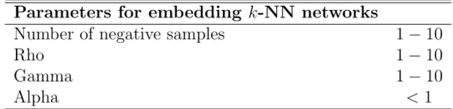
Before implementing viSNE [8] and our method, we need to set the parame-ters of each method. viSNE is based on Barnes-Hut-SNE [28], which has two parameters: perplexity and theta that controls the tradeoff between speed and accuracy. In our experiments, we set the two as 30 and 0.5, respectively, which were the values the authors of viSNE used. Our method allows for more control and therefore has more parameters: number of trees, number of neighbors, perplexity, number of negative samples, rho, gamma, and al-pha. We set the parameters considering our input data set. The first three parameters are related to constructing ak-NN network. The number of trees and neighbors can determine the shapes of ak-NN network, and perplexity is related to computing edge weights of Equation (2.2). The other parameters are related to network embedding. The number of negative samples is M of Equation (2.5), rho is the initial learning rate, gamma is the weight of negative edges, and alpha determines the thickness of the tail off. Table 3.1 and Table 3.2 show the parameters we tuned for our visualization.
Table 3.1: Parameters for constructing k-NN networks. Parameters for constructing k-NN networks
Number of trees 20−100
Number of neighbors 20−150
Perplexity 10−50
Table 3.2: Parameters for embedding the constructed k-NN networks. Parameters for embedding k-NN networks
Number of negative samples 1−10
Rho 1−10
Gamma 1−10
Alpha <1
3.3.2
Hardware Details
All experiments for measuring the computation time were performed on a machine with Intel Xeon E5-2650 CPUs running at 2.30GHz and 512GB memory. 40 threads were used, except in the experiments about the effec-tiveness of multiple threads.
CHAPTER 4
RESULTS
4.1
Visualization
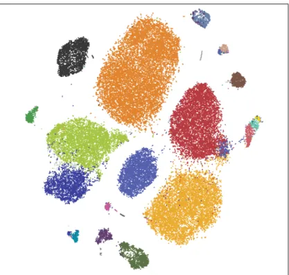
Figure 4.1 represents the visualization result for mice bone marrow replicate 7 data set [12]. Overall, the same type of cells forms a dense subset. The number of a certain class of cells such as hematopoietic stem cell (HSC) in the data set was so small that they were difficult to distinguish from other cell types and to find in our visualization. Except for these cells, we can clearly see that cells of the same type gather together and cells of different type move away from each other in a two-dimensional space.
We can also find some similar kinds of cells staying together in Figure 4.1. For example, similar cell types like Intermediate Monocytes (red) and Classical Monocytes (yellow) appear close to each other. Two types of B cells (purple and light green) also stay near with each other.
Figure 4.1: Visualization of our metho d for the data set whic h con tains mice b one marro w replicate 7.
In addition, we applied viSNE to the same data set. Figure 4.2 shows that viSNE can also represent cell subpopulation heterogeneity very well. Cells of the same type are grouped together and can be clearly distinguished from different types of cells. In the context of the shape of subpopulations in the visualization, our method tended to form denser and rounder clusters than viSNE but to have more randomly scattered samples. We also compared our method with other embedding methods such as PCA. Some examples of the PCA visualization are shown when we introduce our web-based interactive system (see Chapter 5).
Figure 4.2: Visualization of viSNE for the data set which contains mice bone marrow replicate 7.
4.2
Computation Time
One of the main goals of our method is to make visualization of high-dimensional single-cell data faster and more scalable. Thus, we compared the computation time of viSNE [8] and our method for various cases. In addition, to test the scalability and parallelizability, we measured the effec-tiveness of speedup with respect to the number of threads.
4.2.1
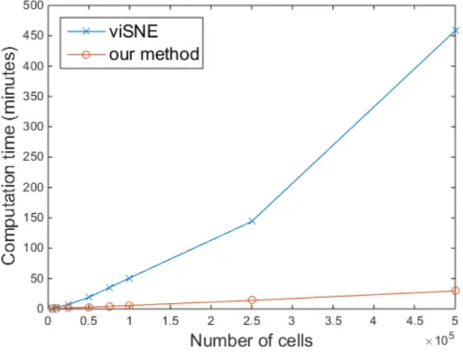
Time Comparison Depending on the Number of Data
To measure the computation time and evaluate the scalability with respect to the size of the data sets, we constructed 8 different single-cell data sets that contained 5,000, 10,000, 25,000, 50,000, 75,000, 100,000, 250,000, and 500,000 data points, respectively. For each data set, single-cell data points were uni-formly sampled from the union of 10 data sets (total number: 841,644). Each data set contained 39 parameters and was preprocessed by noise thresholding and asinh transformation before sampling. Figure 4.3 shows that our method was faster than viSNE for all 8 sampled data sets and our method is easier to make scalable. In addition, our method is still efficient beyond the technical limitation of viSNE, 100,000 samples.
Figure 4.3: Comparison of the computation time of viSNE and our method with respect to the number of single-cell data samples.
4.2.2
Computation Time Comparison for Each Step
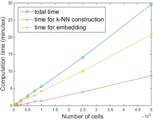
The total computation time of our method consists of two parts: one is for constructing a k-NN network and the other is for embedding the network. In
Figure 4.4, we represent how much time is needed for each step. We can show that the second step, embedding, requires more computational burden. The gap between two steps is widening when the number of single-cells increases.
Figure 4.4: Separate analysis of the computation time for constructing a k-NN network and for embedding the network with regard to the number of single-cell data samples.
4.2.3
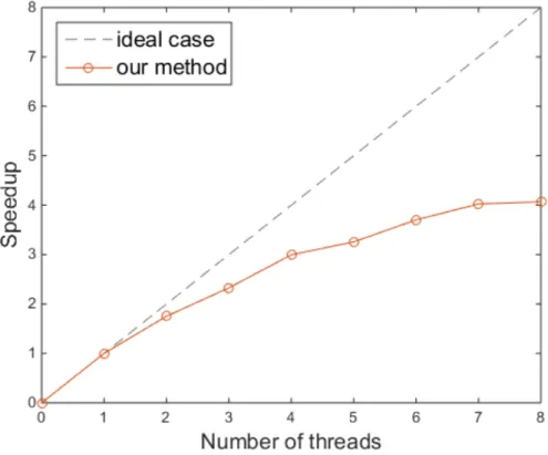
Effectiveness of Parallelization
In addition, we tested the parallelization of our method in the multi-core setting. Since our method uses asynchronous stochastic gradient descent (ASGD) [33] for training, it can be implemented in parallel by using multiple threads and be easily accelerated. We measured the computation time of our method when dealing with the union of all 10 single-cell data sets with respect to the number of threads. By increasing the number of threads from 1 to 8, we measured the effectiveness of the multiple threads for our method. When we used 8 threads simultaneously, the speedup rate was 4.1 times faster than the single thread implementation, which is shown in Figure 4.5. The results
show that our method can be effectively parallelized and can be made more scalable through a multi-core system.
Figure 4.5: Effectiveness of the multiple threads for speedup of our method.
4.3
Clustering
In this section, we compared the quality of embedding by comparing the performance of clustering. In our experiments, we first applied one of the off-the-shelf clustering algorithms, k-means clustering [24], to the vectorized single-cell data points embedded by viSNE [8] and by our method. Next, we measured the performance of clustering using hand-gated annotations of each cell. Specifically, we followed the process of X-shift [12], which compares the clustering results and hand-gated populations and calculates F1-measures.
4.3.1
Evaluation of Clustering
In detail, contingency matrix C was obtained for each cluster using hand-gated annotations. The element Cij of the matrix is the number of cells in the ith cluster belonging to the jth population. Based onCij values, we can compute precisionP and recallR: Pij =Cij/P
kCik andRij =Cij/
P
kCkj. By combining two matrices, the F1-measure matrix can be obtained asFij = 2PijRij/(Pij +Rij).
As the number of clusters changed from 2 to 100, we computed F1-measures for each cluster. The F1-measures were used to find a one-to-one assign-ment between hand-gated population and clusters using the Hungarian al-gorithm [40], which maximized the sum of F1-measures. This process was applied to our 10 data sets, and we obtained an average F1-measure sum. As another performance measure, we obtained maximum F1-measures for each data set across all the clusters and took a median.
4.3.2
Performance of Clustering
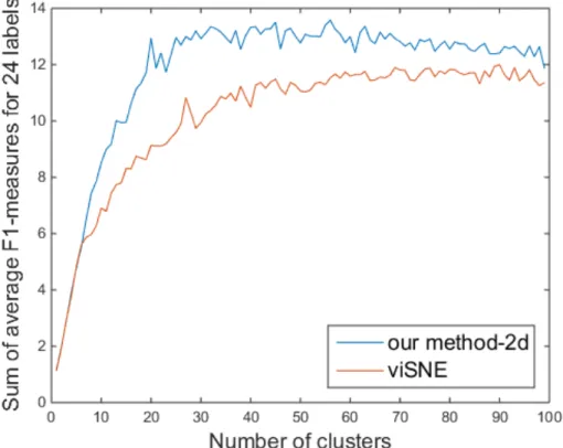
As the input of clustering, we used the two-dimensional vectors obtained by viSNE [8] and our method. We compared an average F1-measure sum of both methods and a median of maximum F1-measures. Figure 4.6 shows that the clustering performance of our method is better than that of viSNE across all the clusters with respect to an average F1-measure sum. In addition, we compared a median of maximum F1-measures of viSNE and our method. Our two-dimensional embedding obtained 14.68 while viSNE obtained 13.23 as its median. Our method also outperformed viSNE for this evaluation metric.
Figure 4.6: Comparison of the clustering performance of viSNE and our method when using two-dimensional vectors with respect to the number of clusters.
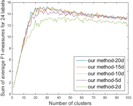
Since our method is developed mainly for visualization, two- or three-dimensional vectors are usually used as a result of embedding. However, the algorithm can embed high-dimensional single-cell data into an arbitrary low-dimensional space other than a two- or three-low-dimensional space. The vectors embedded in a higher-dimensional space than a space for visualization can lose less intrinsic information that original high-dimensional single-cell data have. These higher-dimensional embedded vectors can be used to enhance the performance of clustering. Thus, we tested clustering performances of our embedding using 5-, 10-, 15- and 20-dimensional representations obtained by our method.
As expected, Figure 4.7 shows that the performance of clustering was im-proved when we used the vectors with higher dimensions than two. The performances as we used 10-, 15-, and 20-dimensional vectors are similar to each other and better than the performance as we used two- or 5-dimensional vectors. This empirically shows that our low-dimensional representations can
be used for purposes other than visualization, such as classification.
Figure 4.7: Comparison of the clustering performance of viSNE and our method when using two-dimensional vectors with respect to the number of clusters.
CHAPTER 5
WEB-BASED INTERACTIVE
VISUALIZATION
To better aid analysis, we also introduce an interactive web browser based vi-sualization tool featured in Figures 5.1 and 5.2. It allows researchers to exam-ine their own data quickly by enabling functionality like mouse-over, zoom, pan, brushing, and linking on the embedded data. Users can color data by quantities of marker values as well as qualitative gate information. One can select arbitrary groups of single-cell data points, tag them, and save them for downstream analysis. We provide code, documentation, and video demon-strations to reproduce experiments and apply our methods to new single-cell data through the link (https://github.com/juhokim/SVHD-Single-Cell). All code is made available under an MIT license.
Figure 5.1 shows the comparison between different visualization methods by using two parallel plots and the reproduced results of our method using the web-based visualization system. The left figure is the visualization result of PCA, which cannot properly distinguish different cell subpopulations while the right figure, our reproduced visualization (the same result as the Figure 4.1.), works well.
Figure 5.1: Compare different visualization methods and reproduce visualization results based on our web-based tool.
plot depicts the result of our proposed method, and the middle plot is a PCA projection of the data. The right plot describes embedded expressions of a specific marker with respect to a certain projection. Color assignment and data selection labeling are also available through widgets at the bottom left. Some data statistics and the table to the right show all provided marker data and meta data regarding the single-cell data.
Figure 5.2: Our web-based system can compare the results from different embeddings and show visualization statistics.
CHAPTER 6
CONCLUSION
In this thesis, we introduced a new visualization method for large-scale and high-dimensional single-cell data based on LargeVis [29], which consists of two parts: constructing an approximate k-NN network and embedding the constructed network into a low-dimensional space. Since both steps have lin-ear time complexity, our method is scalable and suitable for analyzing large-scale single-cell data sets with hundreds of thousands or even millions of cells. Specifically, our experiment results showed that the proposed method is much faster than viSNE [8], a state-of-the-art single-cell visualization method. In addition, through the experiments with clustering, we showed that the qual-ity of our embedding is better than that of viSNE on cell identqual-ity mapping with respect to F1-measures. We also provide a web based interactive vi-sualization tool and all necessary code and documentation to extend this approach to new data.
REFERENCES
[1] O. Stegle, S. A. Teichmann, and J. C. Marioni, “Computational and analytical challenges in single-cell transcriptomics,”Nature Reviews Ge-netics, vol. 16, no. 3, pp. 133–145, Mar. 2015.
[2] F. Buettner, K. N. Natarajan, F. P. Casale, V. Proserpio, A. Scial-done, F. J. Theis, S. A. Teichmann, J. C. Marioni, and O. Stegle, “Computational analysis of cell-to-cell heterogeneity in single-cell RNA-sequencing data reveals hidden subpopulations of cells,”Nature Biotech-nology, vol. 33, no. 2, pp. 155–160, Jan. 2015.
[3] C. Trapnell, D. Cacchiarelli, J. Grimsby, P. Pokharel, S. Li, M. Morse, N. J. Lennon, K. J. Livak, T. S. Mikkelsen, and J. L. Rinn, “The dynam-ics and regulators of cell fate decisions are revealed by pseudotemporal ordering of single cells,” Nature Biotechnology, vol. 32, no. 4, pp. 381– 386, Mar. 2014.
[4] O. Ornatsky, D. Bandura, V. Baranov, M. Nitz, M. A. Winnik, and S. Tanner, “Highly multiparametric analysis by mass cytometry,” Jour-nal of Immunological Methods, vol. 361, no. 1, pp. 1–20, Sep. 2010. [5] S. C. Bendall, E. F. Simonds, P. Qiu, E.-a. D. Amir, P. O. Krutzik,
R. Finck, R. V. Bruggner, R. Melamed, A. Trejo, O. I. Ornatsky, R. S. Balderas, S. K. Plevritis, K. Sachs, D. Pe’er, S. D. Tanner, and G. P. Nolan, “Single-Cell Mass Cytometry of Differential Immune and Drug Responses Across a Human Hematopoietic Continuum,” Science, vol. 332, no. 6030, pp. 687–696, May 2011.
[6] P. Qiu, E. F. Simonds, S. C. Bendall, K. D. Gibbs Jr, R. V. Bruggner, M. D. Linderman, K. Sachs, G. P. Nolan, and S. K. Plevritis, “Ex-tracting a cellular hierarchy from high-dimensional cytometry data with SPADE,” Nature Biotechnology, vol. 29, no. 10, pp. 886–891, Oct. 2011. [7] S. C. Bendall, G. P. Nolan, M. Roederer, and P. K. Chattopadhyay, “A deep profiler’s guide to cytometry,” Trends in Immunology, vol. 33, no. 7, pp. 323–332, July 2012.
[8] E.-A. D. Amir, K. L. Davis, M. D. Tadmor, E. F. Simonds, J. H. Levine, S. C. Bendall, D. K. Shenfeld, S. Krishnaswamy, G. P. Nolan, and D. Pe’er, “viSNE enables visualization of high dimensional single-cell data and reveals phenotypic heterogeneity of leukemia,”Nature Biotech-nology, vol. 31, no. 6, pp. 545–552, May 2013.
[9] S. C. Bendall, K. L. Davis, E.-a. D. Amir, M. D. Tadmor, E. F. Simonds, T. J. Chen, D. K. Shenfeld, G. P. Nolan, and D. Pe’er, “Single-Cell Tra-jectory Detection Uncovers Progression and Regulatory Coordination in Human B Cell Development,” Cell, vol. 157, no. 3, pp. 714–725, Apr. 2014.
[10] K. Shekhar, P. Brodin, M. M. Davis, and A. K. Chakraborty, “Au-tomatic Classification of Cellular Expression by Nonlinear Stochastic Embedding (ACCENSE),”Proceedings of the National Academy of Sci-ences, vol. 111, no. 1, pp. 202–207, Jan. 2014.
[11] M. Setty, M. D. Tadmor, S. Reich-Zeliger, O. Angel, T. M. Salame, P. Kathail, K. Choi, S. Bendall, N. Friedman, and D. Pe’er, “Wishbone identifies bifurcating developmental trajectories from single-cell data,”
Nature Biotechnology, vol. 34, no. 6, pp. 637–645, May 2016.
[12] N. Samusik, Z. Good, M. H. Spitzer, K. L. Davis, and G. P. Nolan, “Automated mapping of phenotype space with single-cell data,” Nature Methods, vol. 13, no. 6, pp. 493–496, May 2016.
[13] B. Anchang, T. D. P. Hart, S. C. Bendall, P. Qiu, Z. Bjornson, M. Lin-derman, G. P. Nolan, and S. K. Plevritis, “Visualization and cellular hierarchy inference of single-cell data using SPADE,” Nature Protocols, vol. 11, no. 7, pp. 1264–1279, June 2016.
[14] A. P. Patel, I. Tirosh, J. J. Trombetta, A. K. Shalek, S. M. Gillespie, H. Wakimoto, D. P. Cahill, B. V. Nahed, W. T. Curry, R. L. Martuza, D. N. Louis, O. Rozenblatt-Rosen, M. L. Suv, A. Regev, and B. E. Bernstein, “Single-cell RNA-seq highlights intratumoral heterogeneity in primary glioblastoma,” Science, vol. 344, no. 6190, pp. 1396–1401, June 2014.
[15] Q. Deng, D. Ramskld, B. Reinius, and R. Sandberg, “Single-Cell RNA-Seq Reveals Dynamic, Random Monoallelic Gene Expression in Mam-malian Cells,” Science, vol. 343, no. 6167, pp. 193–196, Jan. 2014. [16] E. Porpiglia, N. Samusik, A. T. V. Ho, B. D. Cosgrove, T. Mai, K. L.
Davis, A. Jager, G. P. Nolan, S. C. Bendall, W. J. Fantl, and H. M. Blau, “High-resolution myogenic lineage mapping by single-cell mass cytometry,” Nature Cell Biology, vol. 19, no. 5, pp. 558–567, Apr. 2017.
[17] B. Wang, J. Zhu, E. Pierson, D. Ramazzotti, and S. Batzoglou, “Visu-alization and analysis of single-cell RNA-seq data by kernel-based simi-larity learning,” Nature Methods, vol. 14, no. 4, pp. 414–416, Mar. 2017. [18] D. J. McCarthy, K. R. Campbell, A. T. L. Lun, and Q. F. Wills, “Scater: pre-processing, quality control, normalization and visualization of single-cell RNA-seq data in R,” Bioinformatics, vol. 33, no. 8, pp. 1179–1186, Apr. 2017.
[19] F. Buettner, N. Pratanwanich, D. J. McCarthy, J. C. Marioni, and O. Stegle, “f-scLVM: scalable and versatile factor analysis for single-cell RNA-seq,” Genome Biology, vol. 18, pp. 212, Nov. 2017.
[20] D. R. Bandura, V. I. Baranov, O. I. Ornatsky, A. Antonov, R. Kinach, X. Lou, S. Pavlov, S. Vorobiev, J. E. Dick, and S. D. Tanner, “Mass Cy-tometry: Technique for Real Time Single Cell Multitarget Immunoassay Based on Inductively Coupled Plasma Time-of-Flight Mass Spectrome-try,” Analytical Chemistry, vol. 81, no. 16, pp. 6813–6822, Aug. 2009. [21] F. Tang, C. Barbacioru, Y. Wang, E. Nordman, C. Lee, N. Xu, X. Wang,
J. Bodeau, B. B. Tuch, A. Siddiqui, K. Lao, and M. A. Surani, “mRNA-Seq whole-transcriptome analysis of a single cell,” Nature Methods, vol. 6, no. 5, pp. 6813–6822, Apr. 2009.
[22] C. Trapnell, “Defining cell types and states with single-cell genomics,”
Genome Research, vol. 25, no. 10, pp. 1491–1498, Oct. 2015.
[23] L. A. Herzenberg, J. Tung, W. A. Moore, L. A. Herzenberg, and D. R. Parks, “Interpreting flow cytometry data: a guide for the perplexed,”
Nature Immunology, vol. 7, no. 7, pp. 681–685, July 2006.
[24] C. Bishop, Pattern Recognition and Machine Learning. Springer, 2006. [25] H. C. Fan, G. K. Fu, and S. P. A. Fodor, “Combinatorial labeling of single cells for gene expression cytometry,” Science, vol. 347, no. 6222, Feb. 2015.
[26] D. A. Lawson, N. R. Bhakta, K. Kessenbrock, K. D. Prummel, Y. Yu, K. Takai, A. Zhou, H. Eyob, S. Balakrishnan, C.-Y. Wang, P. Yaswen, A. Goga, and Z. Werb, “Single-cell analysis reveals a stem-cell program in human metastatic breast cancer cells,” Nature, vol. 526, no. 7571, pp. 131–135, Oct. 2015.
[27] L. J. P. van der Maaten and G. Hinton, “Visualizing Data using t-SNE,”
Journal of Machine Learning Research, vol. 9, pp. 2579–2605, Nov. 2008. [28] L. J. P. van der Maaten, “Accelerating t-SNE Using Tree-based Algo-rithms,”Journal of Machine Learning Research, vol. 15, pp. 3221–3245, Jan. 2014.
[29] J. Tang, J. Liu, M. Zhang, and Q. Mei, “Visualizing Large-scale and High-dimensional Data,” in Proceedings of the 25th International Con-ference on World Wide Web, 2016, pp. 287–297.
[30] S. Dasgupta and Y. Freund, “Random Projection Trees and Low Dimen-sional Manifolds,” in Proceedings of the Fortieth Annual ACM Sympo-sium on Theory of Computing, 2008, pp. 537–546.
[31] W. Dong, M. Charikar, and K. Li, “Efficient K-nearest Neighbor Graph Construction for Generic Similarity Measures,” in Proceedings of the 20th International Conference on World Wide Web, 2011, pp. 577–586. [32] T. Mikolov, I. Sutskever, K. Chen, G. Corrado, and J. Dean, “Dis-tributed Representations of Words and Phrases and Their Composi-tionality,” inProceedings of the 26th International Conference on Neural Information Processing Systems, 2013, pp. 3111–3119.
[33] B. Recht, C. Re, S. J. Wright, and F. Niu, “HOGWILD!: A Lock-free Approach to Parallelizing Stochastic Gradient Descent,” in Proceedings of the 24th International Conference on Neural Information Processing Systems, 2011, pp. 693–701.
[34] M. Datar, N. Immorlica, P. Indyk, and V. S. Mirrokni, “Locality-sensitive Hashing Scheme Based on P-stable Distributions,” in Proceed-ings of the Twentieth Annual Symposium on Computational Geometry, 2004, pp. 253–262.
[35] M. Muja and D. G. Lowe, “Scalable Nearest Neighbor Algorithms for High Dimensional Data,” IEEE Transactions on Pattern Analysis and Machine Intelligence, vol. 36, no. 11, pp. 2227–2240, 2014.
[36] J. Tang, M. Qu, M. Wang, M. Zhang, J. Yan, and Q. Mei, “LINE: Large-scale Information Network Embedding,” inProceedings of the 24th International Conference on World Wide Web, 2015, pp. 1067–1077. [37] J. Barnes and P. Hut, “A hierarchical O(NlogN) force-calculation
al-gorithm,” Nature, vol. 324, no. 6096, pp. 446–449, Dec. 1986.
[38] M. U. Gutmann and A. Hyv¨arinen, “Noise-contrastive estimation of un-normalized statistical models, with applications to natural image statis-tics,”Journal of Machine Learning Research, vol. 13, no. 1, pp. 307–361, Feb. 2012.
[39] M. H. Spitzer, P. F. Gherardini, G. K. Fragiadakis, N. Bhattacharya, R. T. Yuan, A. N. Hotson, R. Finck, Y. Carmi, E. R. Zunder, W. J. Fantl, S. C. Bendall, E. G. Engleman, and G. P. Nolan, “An interactive reference framework for modeling a dynamic immune system,” Science, vol. 349, no. 6244, July 2015.
[40] J. Munkres, “Algorithms for the Assignment and Transportation Prob-lems,” Journal of the Society for Industrial and Applied Mathematics, vol. 5, no. 1, pp. 32–38, Mar. 1957.