What Makes a Test Score? The Respective Contributions of Pupils, Schools, and Peers in Achievement in English Primary Education

IZA DP No. 3866

What Makes a Test Score?

The Respective Contributions of Pupils, Schools, and

Peers in Achievement in English Primary Education

Francis Kramarz

Stephen Machin

Amine Ouazad

What Makes a Test Score?

The Respective Contributions of Pupils,

Schools, and Peers in Achievement in

English Primary Education

Francis Kramarz

CREST, CEPR, IFAU and IZA

Stephen Machin

University College London, CEE, CEP, CEPR and IZA

Amine Ouazad

INSEAD, CEE, CEP and CREST

Discussion Paper No. 3866

December 2008

Anyopinions expressed here are those of the author(s) and not those of IZA. Research published in this series may include views on policy, but the institute itself takes no institutional policy positions. The Institute for the Study of Labor (IZA) in Bonn is a local and virtual international research center and a place of communication between science, politics and business. IZA is an independent nonprofit organization supported by Deutsche Post World Net. The center is associated with the University of Bonn and offers a stimulating research environment through its international network, workshops and conferences, data service, project support, research visits and doctoral program. IZA engages in (i) original and internationally competitive research in all fields of labor economics, (ii) development of policy concepts, and (iii) dissemination of research results and concepts to the interested public. IZA Discussion Papers often represent preliminary work and are circulated to encourage discussion.

IZA Discussion Paper No. 3866 December 2008

ABSTRACT

What Makes a Test Score?

The Respective Contributions of Pupils, Schools, and

Peers in Achievement in English Primary Education

This study develops an analytical framework for evaluating the respective contributions of pupils, peers, and school quality in affecting educational achievement. We implement this framework using rich data from England that matches pupils to their primary schools. The dataset records all English pupils and their test scores in Key Stage 1 (age 7) and Key Stage 2 (age 11) national examinations. The quality of the data source, coupled with our econometric techniques, allows us to assess the respective importance of different educational inputs. We can distinguish school effects, that affect all pupils irrespective of their year and grade of study, from school-grade-year effects. Identification of pupil effects separately from these school-grade-year effects is achieved because students are mobile across schools. Peer effects are identified assuming variations in school-grade-year group composition in adjacent years are exogenous. We estimate three different specifications, the most general allowing Key Stage 2 results to be affected by the Key Stage 1 school(-grade-year) at which the pupil studied. We discuss the validity of our various exogeneity assumptions. Estimation results show statistically significant pupil ability, school and peer effects. Our analysis suggests the following ranking: pupils' ability and background are more important than school time-invariant inputs. Peer effects are significant, but small.

JEL Classification: I21

Keywords: education, peer effects, school effects, school quality

Corresponding author: Amine Ouazad INSEAD Boulevard de Constance 77300 Fontainebleau France E-mail: amine.ouazad@insead.edu

We would like to thank audiences of various seminars and conferences. In particular, Marc Gurgand, Eric Maurin, Thomas Piketty, Jesse Rothstein suggested helpful improvements. Previous versions of this paper were presented at the May 2006 COST meeting, the Jamboree of the European Doctoral Program, the Lunch Seminar of Paris-Jourdan Sciences Economiques, the Crest internal seminar, the 2006 IZA prize in labor economics conference, the summer research program at Boston College, the networks seminar at Cornell University, the IFAU Seminar at Uppsala University, and the 2008 Annual Meeting of the Society of Labor Economists. The authors acknowledge financial and computing support from the Centre for Economic Performance, the Centre for the Economics of Education, CREST-INSEE, INSEAD, and the Economics of Education and Education Policy in Europe (EEEPE)

1

Introduction

A key question for education policy is which of the many educational inputs - including social background, schools, peers and teachers - really make a difference? Accurately determing an answer is crucial to good decision-making in education. Indeed, in the real world context of limited funding there is a trade-off between a range of education policies like targeting pupils, targeting schools, promoting desegregation, implementing tracking, hiring and promoting good teachers. Choosing between alternative policy strategies very clearly requires some knowledge on the relative impact of schools, pupil abilities, family background and peers on educational achievement. If schools make a difference then changing school inputs, management and teaching practices can enhance educational performance. If, on the other hand, peers are more important, segregation may be the number one issue to tackle. Finally, if pupils’ ability or background - more generally pupil-specific issues - are the principal determinants of achievement, policies targeting low achieving pupils may have the highest potential to narrow achievement gaps between children.

However, there remains no real consensus on what reallymakes a difference despite these issues being hotly debated for a long time (Summers and Wolfe, 1977). This is partly because the questions of how to identify these different effects are very challenging from an empirical viewpoint. This said, there are some stylised facts that emerge from different strands of the literature. For example, scholars in the sociology of education have long argued that, apart from students’ ability and background, peers are the most important determinant of test scores. This dates back at least as far as the Coleman (1966). InThe Concept of Equality of Educational Opportunity(1969), Coleman asserts that:

[...] those inputs characteristics of schools that are most alike for Negroes and whites have least effect on their achievement. The magnitudes of differences between schools attended by Negroes and those attented by whites were as follows: least, facilities and curriculum; next, teacher quality; and greatest, educational backgrounds of fellow stu-dents. The order of importance of these inputs on the achievement of Negro students is precisely the same: facilities and curriculum least, teacher quality next, and backgrounds of fellow students, most.

Following the Coleman report, a series of desegregation programs were initiated – notably busing programs. Furthermore the report sparked a significant research venture on the effects of peers, school quality and pupil backgrounds on achievement (Coleman, 1975; Clotfelter, 1999; Guryan, 2001).

However, a number of papers by economists have challenged some of the key findings from the report and the research literature it stimulated. A seminal paper (Manski, 1993) highlighted the main problems of the baseline specification used by James Coleman. Selection bias is the most important one: if we observe good pupils together, are they good because they are together or are they together because they are good? Students may be partly selected on unobservable

character-effect of peers’ behaviour from the character-effect of peers’ characteristics. The other significant observation is that the econometrician needs to address the issue of simultaneity bias since students influence each other simultaneously. Hoxby (2000a) has estimated the overall effect of race and gender com-position on Texas primary school pupils. She finds significant and large peer-effects. In the context of the Boston METCO desegregation program, Angrist and Lang (2002) estimate the effect of mi-nority students on test scores. Their estimated effects are modest and short-lived. Gould, Lavy and Paserman (2004) assess the impact of immigrants on Israeli pupils. Even though the average effects report are not statistically significant, they do find that low-achieving pupils are more sensitive to their peers.

Another strand of the literature has focused on the relationship between school quality and achievement. Typically school quality has been proxied by various observable indicators like the teacher-pupil ratio, teacher education, teacher experience, teacher salary or expenditures per pupil. Overall, despite it being a controversial and contested issue, the link between school resources and test scores appears to be relatively weak (Hanushek, 1986; Hanushek, 2003; Krueger, 2003). The ‘school effectiveness’ research, carried out mostly by educationalists, comes to a similar conclusion: schools matter, but not by anywhere near as much as non-school factors like the home environment (Mortimore, Sammons, Stoll, Lewis and Ecob, 1988; Stiefel, Schwartz, Rubenstein and Zabel, 2005; Teddlie and Reynolds, 1999; West and Pennell, 2003). In the British context, Levacic and Vignoles (2002) mention that the impact of school resources is small and very sensitive to misspecification. Dearden, Ferri and Meghir (2002) suggest that, while the pupil-teacher ratio has no significant impact, attending selective schools improves both attainment and wages.

In this area Hanushek (1986) has stated

‘Schools differ dramatically in quality, but not for the rudimentary factors that many researchers (and policy makers) have looked to for explanation of these differences.’ (Hanushek, 1986)

In a recent paper, Rivkin, Hanushek and Kain (2005) indeed argue that test scores are the sum of student, school and teacher effects. Since these are potentially unobservable, they strongly argue that analysis should therefore not solely rely on observable characteristics for the estimation of school and teacher effectiveness. However, they do not try to identify all the different components of their favored specification.

Like the innovative Hanushek, Rivkin and Kain work, the focus of our paper is rather different to the peer group and school quality work that tends to focus on a single issue. Rather we attempt to measure the relative contributions of pupils, schools and peers without restricting our analysis to observable proxies for peers’ characteristics or school quality. To do so we set up an empirical framework which enables us to jointly estimate time-varying school fixed effects (school-grade-year effects) and pupil fixed effects. The former are then decomposed into an observable time-varying part (the social composition) and an unobservable school effect.

Our estimation strategy combines ideas from the literature using matched worker-firm data (Abowd, Kramarz and Margolis, 1999) and from work in the economics of education (e.g. Hoxby,

2000a). Our data has pupils matched to the schools they attend over time. Therefore, following Abowd et al. (1999), pupil and school effects are identified using school switchers, assuming in particular that mobility decisions are not motivated by time-varying pupil-specific shocks. Following Hoxby (2000a), we argue that variations in the average quality of pupils within a school across consecutive years are essentially idiosyncratic, because demographics change randomly from year to year around a central tendency. From a methodological standpoint, our paper goes further than the previous literature in at least two important dimensions: (i) it assesses the relative contribution of peers, school quality and pupils’ ability and background using a single equation; and (ii) it estimates the overall effect of peers without relying on specific peer characteristics.

We implement the empirical framework using an extremely rich administrative database on English pupils in state schools. We use three cohorts of English pupils in state schools.1 The dataset follows all pupils from primary to secondary education. England also has a national curriculum with an associated national testing schedule. The outcomes we consider are national test scores (Key Stage 1, taken in Year 2 at age 6/7, and Key Stage 2, taken at the end of primary school in Year 6 at age 10/11). The grades achieved at the end of these Key Stages are particularly important instruments for both parents and the English education authorities. In particular, government uses them to set targets and parents can freely read about them in performance league tables, published on the web or in the popular press.

Our estimation results show pupil heterogeneity to be a more important determinant of achieve-ment than school quality, even though both inputs are statistically significant. Peer effects are mostly small, but also significant. We assess the robustness of our assumptions in a number of ways and examine the mobility patterns in the data, with particular care placed on the reasons for pupil mobility (importantly distiguishing between compulsory moves due to the structure of the English school system and non-compulsory moves). These robustness tests largely confirm that conditioning on person effects and on school-grade-year effects is a reasonable strategy.

The finding that pupil effects matter most is, of course, important in the light of research arguing that early interventions (often pre-school) yield higher educational achievement returns (Heckman and Masterov, 2007). If such policies aimed at dampening down achievement gaps on entry (or early on) in primary school do indeed work best then our findings suggest that this is likely to have an important impact on subsequent gaps and inequalities in educational achievement that occur throughout the compulsory school years. But our findings also show there to be important, albeit smaller, contributions of peers and schools to the variance of pupil achievement and therefore that educational differences do evolve during children’s school careers. Evidently this matters for the design of education policies at different stages of compulsory schooling.

The outline of the rest of the paper is as follows. Section 2 presents the various specifications we consider, as well as the estimation strategy we implement for each specification. In each case, discussion of the specification is related to relevant papers in the associated literature. Section

1

The data are census data on pupils in state schools - this comprises the vast majority of English school children. Only around 7 percent receive their education outside of the state sector in private schools (and the percentage is even lower in the primary schooling stage we study).

3 introduces the reader to the specific English policy context and describes the dataset. Section 4 analyzes the regression results. Section 5 discusses the robustness of the estimation, examines mobility patterns and gives some public policy implications of the results. Section 6 concludes.

2

The Econometric Framework

2.1 Specifications

In this section we introduce the various econometric models from which we extract estimates of the relative importance of different educational inputs. The plan is to empirically implement them in the context of primary school children in England, although of course our approach would (broadly) carry over to other institutional settings.

The compulsory school careers of English children are organised into four Key Stages: Key Stages 1 and 2 which take place in primary school; and Key Stages 3 and 4 in secondary school. Our focus is on primary schools where Key Stage 1 examinations are taken at age 6/7 (grade 2) and Key Stage 2 examinations at the end of primary school at age 10/11 (grade 6).2

To begin note that, as inter alia Rivkin et al. (2005) and Todd and Wolpin (2003) point out, academic achievement at any point in a pupil’s education is a cumulative function of endowments (ability and family background), of school quality, and of the environment (community, in particu-lar). This implies that: (i) test scores are a function of these educational inputs; (ii) these inputs can vary over time; and (iii) educational production functions should include the whole history of inputs that shaped each pupil’s experience. The current section presents four different specifications that incorporate some or all of these features, as depicted below:

yi,f,t=xi,f,tβ+θi+ψJ(i,t)+εi,f,t (SE)

yi,f,t=xi,f,tβ+θi+ϕJ(i,t),g(i,t),t+εi,f,t (SGYE)

yi,f,t=xi,f,tβ+θi+ϕJ(i,t),g(i,t),t+λϕJ(i,t−1),g(i,t−1),t−1+εi,f,t (PSGYE)

And the last specification,

yi,f,t=xi,f,tβ+ (1 +λ(t−1))·θi+ϕJ(i,t),g(i,t),t+λϕJ(i,t−1),g(i,t−1),t−1+εi,f,t (PIE)

In each of these specifications, there are two Key Stage periodst= 1,2,idenotes the N pupils withi= 1, . . . , N;j denotes theJ schools withj = 1, . . . , J. yi,f,tis the test score of pupiliat time

t in examination topic f. J(i, t) denotes the school pupil iattended at time t and g(i, t) denotes the grade in which pupil iattends in yeart.

2_{Ideally, we would like to estimate the model up to key stage 4, but we would need to follow at least two cohorts} from key stage 1 to key stage 4 and currently the dataset follows only one cohort all the way through school careers. Future releases of the National Pupil Database will include multiple cohorts from key stage 1 to key stage 3 and above.

The first specification (SE) is the same as that analysed in the worker-firm study of Abowd et al. (1999). In (SE) the test score is decomposed into a pupil effect θi, a school effectψJ(i,t),xi,f,tβ is the effect of the K time-varying covariates, and εi,f,t the residual3. The covariates are controls for cohorts, years and exam subjects. The main advantage of specification (SE) is its simplicity. However, it does not take into account the fact that school-specific inputs can vary over time. For instance, teachers may be different from one year to the other and the student body of the school changes. To take into account this feature, specification (SGYE) therefore generalises this by positing that achievement is the sum of a student effect and a school-grade-year effect.

Specifications (SE) and (SGYE) remain restrictive in that they assume the only input that affects outcomes at different stages of the educational curriculum is pupil ability. So, for example, the quality of the teachers or the environment at the initial stage does not affect future outcomes. It is likely however that some features of the school (or school-grade-year) that a pupil attended in the past (Key Stage 1, date t−1) have an impact on test scores at datet. This feature is captured in Specification (PSGYE) which states that test scores are the sum of a student effect, the current school-grade-year effect and the past school-grade-year effect discounted by λ. Because we do not observe grades before Key Stage 1, we constrain the initial past school-grade-year effect to be equal to zero, ϕj,g,0 = 0. At this initial date, the school-grade-year effect and the pupil effect θ cannot

be separately identified given the data. Notice that, in the same fashion as in value-added models, this specification constrains the current and past effect of schools to be proportional (Todd and Wolpin, 2003).

Finally, there is one last issue remaining in specification (PSGYE), namely the child’s progress only depends on the school and not on his/her ability. The most general specification (PIE) allows progress of the child to depend both on the child’s ability and his/her past and current schools. It also allows us to assess the long run effect of schools on achievement. If λ is estimated to be nonzero, schools have an effect not only on current achievement but also on achievement in the next period (i.e. grade 6 at the end of Key Stage 2 in our study context).

2.2 Identification Hypotheses

The identification of specifications (SE), (SGYE), (PSGYE), (PIE) requires bothsufficient mobility

andexogeneous mobility, both of which are defined in this sub-section, in addition to the traditional exogeneity of the other covariates. In addition to this, we will assume that at least one of our specifications is correct. For instance, if the true model involves a pure match effect, namely an unobserved component specific to both the pupil and the school because, say, some schools are better suited to more able pupils, then our estimates would have no clear meaning. We need to rule this possibility out.4

3

Of course, in Abowd et al. (1999) the effects were firms (our schools) and workers (our pupils).

4_{Education is an interaction between teachers and students, between schools and students. It is therefore quite a} limitation of fixed effects models that they do not allow for complementarities between schools and students. This is very much ongoing research. Woodcock (2007) and Woodcock (2008) estimate a model of wage decomposition with worker, firm and match effects, at the cost of additional assumptions on the correlation structure between match

Notations: i, i0, i00 are pupils. j, j0, j00, j000 are schools or school-grade-years. Reading: iconnects schoolj and

schoolj0 because iattends schoolj in the first period, andiattends schoolj0 in the second period.

Figure 1: (a) Sufficient mobility – The mobility graph has only one connex component. (b) Mobility is not sufficient – The mobility graph has two connex components, {j, j0} and {j00, j000}.

Mobility is defined as sufficient when the mobility graph for pupils and schools is connected (Abowd et al., 1999; Abowd, Creecy and Kramarz, 2002). Two schools are connected if and only if at least one pupil has attended both schools in different years. The set of all these connections is the mobility graph, and we say that it is connected when it has only one connex component. This is illustrated in figure 1.

Moreover, exogeneity assumptions specific to our model with pupil and school effects are re-quired (Abowd et al., 1999; Abowd et al., 2002). A threat to identification arises if, for instance, unmeasured unemployment shocks affect mobility and have an effect (e.g. through reduced income) on outcomes (Hanushek and Rivkin, 2003). For this example, assume those families who experience an unemployment shock between the two periods are more likely (i) to make their child move to a bad school and (ii) to experience lower test scores due to their parents’ joblessness, then the difference between bad and good schools might be underestimated.

To better understand why sufficient and exogenous mobility are jointly needed, consider the set of pupils who attend schooljin period 1 and schoolj0 in period 2. This mobility is clearly necessary since these movements allow the identification of the relative effectiveness of school j with respect to schoolj0. Ignoring the effect of covariates for the sake of clarity, this gives:

E[∆yi,f|i, J(i,2) =j0, J(i,1) =j] = ψj0−ψ_j

+ E[∆εi,f|i, J(i,2) =j0, J(i,1) =j] (1) with ∆yi,f =yi,f,2−yi,f,1 and ∆εi,f =εi,f,2−εi,f,1. With exogenous mobility,E[∆εi,f|i, J(i,2) =

j0, J(i,1) =j] = 0, the last term of the sum drops. This is potentially where unemployment shocks, divorce, etc. could make trouble. Exogenous mobility rules this possibility out. Now, given this assumption, ifψj is identified then ψ0j is identified.

It is then easy to see that when the mobility graph has only one connex component, choosing one arbitrary school and one arbitrary pupil ıand setting their effects ψ andθı to zero identifies all school and pupil effects. A formal definition of the mobility graph and the identification of the model are detailed in appendix A.

So far our intuition has been built on the simplest specification SE. Introducing school-grade-year effects in specifications (SGYE) and (PSGYE) not only allows more flexibility in the measure-ment of school effectiveness, it also introduces more pupil mobility, since pupils necessarily change year-group between the two periods. In addition, because school-grade-year effects time-vary, the exogeneity assumptions are weaker than before. Model (SGYE) is a particular case of (PSGYE) in which the discounting factor is set to 0. Again, identification conditions are identical.

2.3 Identification of Peer Effects

Once we have estimated school-grade-year effects, we would also like to disentangle the effect of the social composition of the school-grade-year from the other inputs under plausible identifying conditions. Identification of such peer effects is challenging. The main issues are described in Manski (1993). First, students may be sorted partly based on unobservable characteristics – for instance, teachers and students may not be randomly matched. Second, students influence each other which means it is hard to disentangle the effect of one on the other; in other words, there is a simultaneity bias. And third, it is hard to identify the effect of peers’ characteristics from the effect of peers’ behaviour.

We assume, as in Hoxby (2000a) and Gould et al. (2004), that the year-to-year variations in school-grade-year composition are exogenous, essentially because of the randomness of the demo-graphics. For instance, in the case of ethnic peer effects, plus or minus one black caribbean student in a given year is probably an idiosyncratic variation. We therefore regress the school-grade-year effect on a school identifier and the composition of the school-grade-year.

ϕj,g,t =ψj + ˆE(z|j, g, t)γ+νj,g,t (2) For each school-grade-year j, g, t, ˆE(z|j, g, t) denotes the vector of average student characteristics, for instance the fraction of boys, the fraction of blacks, the fraction of free school meal students. This strategy is likely to capture most of the bias due to non-random sorting of students between schools, essentially assuming that there is no correlation between changes in school-grade-year composition and unobservable school inputs.

Formally, year-to-year variations in school-grade-year student composition should be exogenous conditional on the school-by-grade fixed effect. Variations in school-grade-year composition should

not be correlated with unobserved time-varying school characteristics.

E[νj,g,t=2−νj,g,t=1|Eˆ(z|j, g, t= 2)−Eˆ(z|j, g, t= 1)] = 0 (3)

ˆ

E(z|j, g, t = 2)−Eˆ(z|j, g, t = 1) is the year-to-year variation in school-grade-year composition.

νj,g,t=2−νj,g,t=1 represents unobserved time-varying shocks in school quality.

This hypothesis adresses the issue of the selection bias. The simultaneity bias is adressed through the use of a common school-grade-year effect for all students. Students “share” the same local public good, which includes peer-effects.

However we are not able to separately identify the effect of peers’ characteristics and the effect of peers’ behaviour. Thus the vector of social interactions γ captures both of these peer-effects. Thus in (6) γ is the reduced form peer-effect.

2.4 Decomposing Inequalities

The models we have specified allow us to decompose inequalities of test scores and test score gaps into components attributed to schools, peers and pupils’ ability and background. We can do this since test scores are the sum of the pupil effect, the year-group effect and the past year-group effect. In our KS2 and KS1 models, these can be written:

y2 = θ+ϕ2+λϕ1+ε2

y1 = θ+ϕ1+ε1

where indices have been dropped for the sake of clarity. Moreover, school-grade-year effects can be decomposed into a permanent school effect and the effect of school composition:

ϕ=ψ+zγ+ν

Inequalities of educational achievement can therefore be decomposed into inequalities of school quality, inequalities of pupil ability and background, and inequalities due to different social contexts, for instance stemming from varying patterns of segregation. In the first period:

V ar(y1) =Cov(y, θ) +Cov(y, ϕ1) +V ar(ε1)

The first term is the component due to pupils’ differences in ability and background. It is the sum of the heterogeneity in pupil ability and background, and the matching between pupil ability and school-grade-year quality, i.e. Cov(y, θ) =V ar(θ) +Cov(θ, ϕ). The same decompositon applies to school-grade-years,Cov(y, ϕ) =V ar(ϕ) +Cov(θ, ϕ). Hence, school-grade-year quality can widen inequalities in test scores if (i) school-grade-years are heterogeneous (ii) good pupils – high-θpupils – are matched with good school-grade-years. Matching good school-grade-years to low-θ pupils should reduce inequalities.

This match between good school-grade-years and low-θ pupils can take two routes: (i) by fos-tering desegregation, i.e. decreasing Cov(γz, θ); and/or (ii) by matching high-ψschools with low-θ

pupils.

2.5 Other Identification Methods Used in the Associated Literature

This section compares the identification strategy of this paper with the identification strategies that have been introduced in past literature. We first compare our models to the value-added models that are used in many papers on the measurement of school effectiveness. A seminal paper (Rivkin et al., 2005) uses this model to emphasize the importance of teacher effects on academic achievement. Finally, we compare the identification strategy of our paper to hierarchical linear models that have flourished in the educational literature.

i) Value Added Models

In value added models, the outcome variable is the progress of the pupil rather than the absolute test score. This basically corresponds to a dynamic panel data model in which the coefficient on the lagged outcome is constrained to be equal to 1, i.e. λ= 1 in specification PIE. The results of our estimations and of value added models are comparable.

A value added model would decompose the progress of the child into a child fixed effect, a school-grade-year effect and a residual.

∆yi,f,t=xi,f,t·β+θi+ϕJ(i,t),g(i,t),t+ui,f,t (4)

where ∆yi,f,t= yi,f,t−yi,f,t−1 is the progress of the child between two subsequent periods. Other

notations are as before. xi,f,tis a vector of time-varying controls. There are two differences between this model and specification PIE: (i) the value added model is more restrictive as it constrains the effect of past achievement on current achievement so that λ = 1, and (ii) the error structure in the value-added model is such that time varying unobservables can have long-term consequences on achievement. Indeed, the value-added specification can be rewritten as:

yi,f,t=xi,f,tβ+xi,f,t−1β+ 2·θi+ϕJ(i,t),g(i,t),t+ϕJ(i,t−1),g(i,t−1),t−1+ui,f,t+ui,f,t−1 (5)

This model is equivalent to specification PIE when λ= 1 and ui,f,t+ui,f,t−1 =εi,f,t. Thus value-added models are equivalent to our model with a decay rate of 1, up to the error structure. Point estimates should therefore be equal in both models. Our results reported below suggest that teacher effects are robust to a range of decay rates λ. Thus estimated effects from the value added model and our full model should be similar.

ii) Teacher Effects: Rivkin et al. (2005)

Rivkin et al. (2005) specify an educational production function in which student value-added is decomposed into a student effect, a school effect and a teacher effect. In our notation,

∆yi,f,t=θi+ψJ(i,t)+τT(i,f,t)+εi,f,t (6) where ∆yi,f,t is the gain in student achievement of studenti, in fieldf in yeart. This specification adds a teacher effect τT(i,f,t) where T(i, f, t) is the teacher of studentiin field f in year t. In their

paper, Rivkin et al do not identify all the effects, but rather use this specification as a blueprint and then estimate bounds for the variance of the teacher effects.

Specification (6) is remarkable in a number of ways. First, it does not include school-grade-year effects. Second, it includes teacher effects, which is an addition to specification (SE) of our paper. School effects ψJ(i,t) will not capture year-to-year variations of the student body, and the teacher

effect τT(i,f,t) is likely to include both time-varying teacher quality and year-to-year variations of

the student body that are correlated with changes in teacher quality.

iii) Metropolitan Area Fixed Effects: Hanushek and Rivkin (2003)

In Hanushek and Rivkin (2003), educational progress is decomposed into a family effect and a metropolitan area fixed effect.

∆yi,f,t=θi+θi,t+M SAM(i,t)+εi,f,t (7) where ∆yi,f,t is the gain in student achievement of student i in topic f in year t. M SAM(i,t)

is a metropolitan area fixed effect, where M(i, t) is the metropolitan area of student i in year t. Estimation is carried out on Texas data, which contains 27 MSAs.

Three features of specification (7) are noticeable: first, student effects can vary over time; second, school effects nor school-grade-year effects are present; and last, metropolitan area fixed effects do not vary over time. These elements have the following consequences. Student time-varying fixed effects are likely to capture other time time-varying inputs such as the metropolitan area social composition. Metropolitan area fixed effects are likely to capture public good quality and average school quality in the area, but not year-to-year variations of the social composition of the area.

iv) Hierarchical Models for the Analysis of School Effects

Empirical work in education has used hierarchical linear models in several papers, notably in Rau-denbush and Bryk (1986), Bryk and RauRau-denbush (1992), Goldstein (2002) or Rao and Sinharay (2006). These models identify individual effects, school effects and potentially teacher effects using only cross-sectional data. Despite its light data requirements, an important limitation of multilevel modelling is that they nest individual effects, school effects and other determinants of educational

achievement. Our model does not, since it uses pupil mobility to identify the effects. Multilevel models are written as a set of specifications at multiple levels, e.g. a student level equation and a school level equation. Equations are then combined to lead to a single specification.

Another drawback is that Raudenbush and Bryk (1986) and Bryk and Raudenbush (1992) specify

random effects and not fixed effects. The identification of random effects require the assumption of strict exogeneity, which implies that, for instance, school effects are orthogonal to covariates and to other random and/or fixed effects (Wooldridge, 2002, p257). It is likely that, for instance students with a high or a low effect go to particular schools, or that schools with a good intake are particular schools. Thus it is unlikely that the orthogonality between the effects and covariates is a realistic assumption.

2.6 Estimation Method

The estimation of the model presented in this section cannot proceed in the same way as usual Ordinary Least Squares estimation techniques. The number of right-hand side variables is the sum

J −1 +N+K of the number of school effects, pupil effects and the number of covariates.5 Usual packages try to invert the matrix of covariates which is time consuming and numerically unstable. Abowd et al. (2002) have therefore developed an iterative estimation technique to estimate the baseline fixed effects model of equation SE. However, specifications with past and current school or school-grade-year effects required new identification proofs and estimation techniques.

The estimation proceeds in the following way: first, it starts by computing the variance-covariance matrix of the model with dummies and covariates. This a large and sparse matrix. Second, starting with a first guess for fixed effects and coefficients – usually zero –, the procedure iterates by updating the approximate solution. The sequence of approximate solutions is obtained by the conjugate gradient algorithm, that converges to the true solution if and only if the variance covariance matrix is invertible; this requires that the mobility graph has one connex component and that the covariates are linearly independent. More about the conjugate gradient can be found in Dongarra, Duff, Sorensen and van der Vorst (1991). Details of the computation of the variance-covariance matrix are given in Appendix B and these computation techniques have given birth to a set of programs developed by the authors and are freely available on the website of the Cornell Institute for Social and Economic Research.

3

Dataset and Estimation Method

3.1 The English Educational Context

The English educational system currently combines market mechanisms (many of which were in-troduced in the Education Act of 1988) in different types of schools with a centralized assessment operating through a National Curriculum (Machin and Vignoles, 2005). Therefore it has the

ad-5

vantage of providing us with fairly different management and funding structures and, at the same time, national exam results for all students.

The assessment system features a National Curriculum which sets out a sequence of Key Stages through the years of compulsory schooling: in primary school Key Stage 1 (from ages 5 to 7) and Key Stage 2 (from ages 7 to 11); and in secondary school Key Stage 3 (from ages 11 to 14) and Key Stage 4 (from ages 14 to 16). At the end of each Key Stage, pupils are assessed in the core disciplines: Mathematics, English and Science (not for Key Stage 1). These tests are nationally set and anonymously marked by external graders.

The English primary schooling system is also characterised by a variety of different management structures and funding sources. Community schools and voluntarily controlled schools, which cater for more than half of the student body, are controlled by the Local Education Authority (LEA), of which there are 150 in England. In the case of community and voluntarily controlled schools, the LEA owns the buildings and employs the staff. On the other hand, in voluntary aided and foundation schools, teachers are employed by the school governing body and the LEA has no legal right to attend proceedings concerning the dismissal or appointment of staff.6 Funding also varies across school types. While most state schools are funded by the government, voluntary aided schools contribute around 10% of the total capital expenditure. These management and funding differences are likely to generate various kinds of incentives, and thus different educational outcomes for pupils.

3.2 The National Pupil Database

The National Pupil Database (NPD) is a comprehensive administrative register of all English pupils in state schools. Data is collected by the Department for Children, Schools and Families and it is mandatory for all state schools to provide accurate data on pupils, who are followed from year to year through a Pupil Matching Reference. Thus panel data can be built by stacking consecutive years of the National Pupil Database.

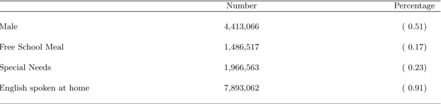
The dataset provides rich information on pupils’ characteristics: gender, free school meal status, special educational needs, and the ethnicity group. Pupils who receive free meals are the 15 to 20% poorest pupils. The ethnicity variable of our sample encodes the main ethnic groups: White, Black Caribbean, Other Black, Pakistani, African Black, Mixed background, Bangladeshi, Indian, Chinese, Other Background.7 It also provides some information on school structures and types (i.e. whether they are community schools, foundation schools, voluntary aided or voluntary controlled schools, and so forth).

Test scores in English, Maths and Science are available - the latter Science test only for Key Stage 2. These tests are externally set and marked. We have standardized test scores to a mean of 50 and a standard deviation of 10 to make results comparable from one level to the other and from year to year.

The structure of the panel data we have built from the NPD is shown in Table 1.

6_{Code of Practice on LEA Schools Relationships, DfES 2001} 7

Coding of the ethnicity variable has changed in the period we consider. It was therefore necessary to recode it in a time-consistent manner.

4

Main Results

We now come to the policy questions of the introduction: do schools matter? do peers matter? are different schooling structures important?

4.1 Pupil, School and School-Grade-Year Effects

Do schools matter? Over the years, this question has been extensively discussed in the sociological and educational literature as well as in recent papers in the economics of education (Rivkin et al., 2005). Our new method of estimating school-grade-year effects and individual effects specifications gives us a new opportunity to re-assess this important question, based upon the extremely rich English data we study.

The estimation of specifications SE to PIE yields pupil fixed effects, school-grade-year effects and school effects. School-grade-year effects are not available for the simple school effects model (specification SE). Some very clear stylized facts come out from considering the correlations and variances/covariances reported in Tables 4 and 5: (i) first of all, pupils are much more heterogenous than either school or school-grade-years effects (ii) individual effects explain a much larger share of the variance of test scores than school or school-grade-year effects.

The first key finding is of a higher variation of pupil fixed effects as compared to school-grade-year effects and school effects can be seen from the Tables, where the standard deviation of pupil effects is between 3.8 and 4.8 times larger than the standard deviation of school effects. Thus, perhaps not surprisingly, suggests that pupils are more heterogeneous than schools. The same finding, of a higher variation, is also true when comparing the standard deviation of pupil effects and the standard deviation of school-grade-year effects. Nevertheless, pupil fixed effects are less precisely estimated than school-grade-year effects or school effects. Indeed, at most five observations per child are available whereas on average 250 observations per school-grade-year are available. To address this potential issue, we look at the correlation between test scores and the school or school-grade-year effects. Individual effects are imprecisely estimated but this should actually lower the correlation between individual effects and test scores.8

The correlation between test scores and individual effects is seen to be between 0.79 and 0.83. This is between 5 and 6.7 times larger than the correlation between school effects and test scores. Indeed, the covariance Table 5 confirms the explanatory power of pupil effects to be much larger than the explanatory power of school effects. This is no surprise given the high correlation, the low variance of school effects and the much higher pupil heterogeneity.

Therefore these baseline results strongly suggest that pupil effects are a more important de-terminant of test scores than school effects. How can one interpret these pupil effects? From our perspective, it seems reasonable to think of them as picking up the whole range of educational ex-periences before age 7: this includes parental background, childcare and kindergarten. Considered in this way, the fact that pupil effects explain most of the variance of test scores is in line with some

of the important contributions to the recent economics of education research area (including, inter alia, Heckman and Masterov (2007), Currie (2001) and Garces, Thomas and Currie (2002)).

4.2 Pupil Effects: Disentangling Individual Effects From Peer Effects and School

Quality

Of course, pupil effects can be correlated with a range of individual characteristics (like ethnicity, gender, free school meal status, special needs and the child’s month of birth) and so an important research challenge is to try to disentangle them from other factors like peer effects and school quality. Doing so differs from an analysis of raw test scores since, under maintained assumptions, it looks at pupil effects free of peer effects and free of the correlation between school quality and observable characteristics.

From our analysis it is evident that pupil effects are reasonably well explained by observable characteristics. For example, the R-Squared from regressions of the fixed effects on observable char-acteristics is around 40% (Table 6). In these regressions, the estimated coefficients are remarkably robust to different specifications. Moreover, the results are in line with descriptive statistics on test scores. The pupil fixed effects of free school meal children are 40 to 41% of a standard deviation lower. Family disadvantage is important, with free school meal pupils being the 10 to 20% poorest children in England. Chinese pupils are the best performing pupils, with a fixed effect 16% of a standard deviation higher than white pupils. Interestingly, Indian pupils have a lower fixed effect than white pupils (6.4 to 7.8% of a standard deviation lower), whereas the test scores of Indian pupils are higher than the test scores of whites. This suggests that basic descriptive statistics do not disentangle the effect of ethnicity from the effect of peers and the effect of school quality. Finally, male pupils have a higher fixed effect, by 2.5 to 2.6% of a standard deviation. This is certainly due to the fact that regressions were carried out by pooling all subjects together. Boys in primary school are better at mathematics and science, whereas girls are better at English. There are therefore around three observations for which boys are better – maths in grades 2 and 6, science in grade 6 – and 2 observations for which girls are better – English in grades 2 and 69.

Table 6 confirms that pupil effects are well explained by observable characteristics, even if one is unable to offer a causal interpretation to the reported findings. The coefficients in Table 6 prove to be very consistent with basic descriptive statistics and, at the margin, this analysis allows us to disentangle pure individual effects from the social context working through peers and school quality.

4.3 Effects of Social Composition on School Quality

As discussed in Section 2.3, the effect of the gender, ethnic and social composition of the school on its quality can be identified under the assumption that year-to-year variations in school composition are exogenous(Hoxby, 2000a; Hoxby, 2000b; Lavy and Schlosser, 2007). Two stylized facts emerge from the covariances in Table 5 and from regressions of school-grade-year effects on school composition

9_{Another version of the tables, available upon request, discarded science test scores. Male fixed effects are then} not significantly higher.

and school effects reported in Table 7: (i) the covariance between school-grade-year effects and test scores is comparable to the covariance between school effects and test scores; and (ii) some of the peer effects are significant but small – effect of the fraction of boys, free meals and special needs. Overall, results suggest peer effects to be statistically significant, but relatively small in magnitude. Looking at the covariances in Table 5 shows the covariance between test scores and school effects to be very similar to the covariance between test scores and school-grade-year effects; 5.6 vs. 7.7 for the school-grade-year specification, 4.6 vs. 4.2 for the past and current school-grade-year specification, and 4.7 vs. 4.0 for the full-fledged specification. Since school-grade-year effects can be decomposed into the school effect and the effect of social composition, these figures imply that peer effects are likely to be less important than school quality.

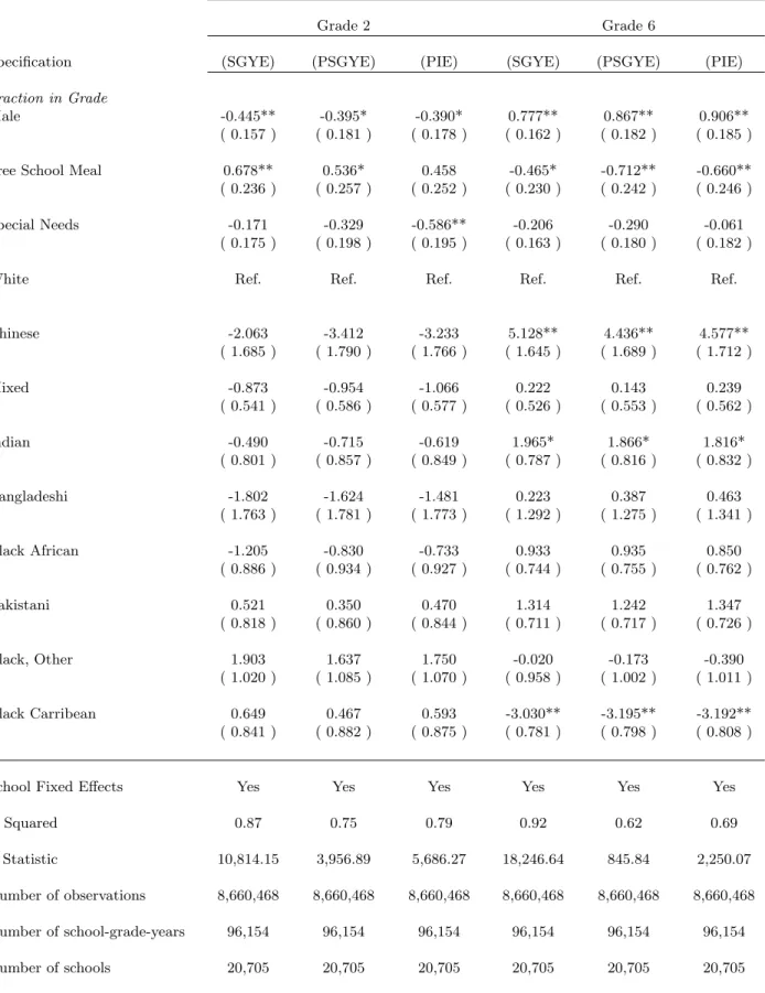
Table 7 shows estimates of the effect of the fraction of different social groups on school-grade-year effects, separately for grade 2 and grade 6. In grade 2, in the full-fledged specification, increasing the fraction of male students by 10% makes school-grade-year effects fall by 0.4% of a standard deviation10 (Table 7, column 3). This effect is robust to different specifications. In grade 6, the effect of the fraction of boys is positive, i.e. increasing the fraction of boys by 10 percentage points increases test scores by 0.9% of a standard deviation (Table 7, column 6). The difference between grade 2 and grade 6 gender composition effects is likely to be due to the fact that grade 2 exams are in English and Maths, whereas grade 6 exams are in English, Maths and Sciences. Boys are better than girls in both science and maths, but not better in English. This effect is robust to the inclusion of past school-grade-year effects and past individual effects in the baseline specification. Most papers in the literature find a negative effect of boys on achievement both in English and in Maths, e.g. Hoxby (2000a).

The fraction of free meal children has a detrimental effect on school-grade-year effects in grade 6; increasing the fraction of free meal children by 10 percentage points lowers school-grade-year effects by 0.7% of a standard deviation (Table 7, column 6).

In grade 6, ethnic composition has an effect on school quality. Chinese and Indian children exert a positive contextual effect, black caribbean children exert a negative contextual effect. The effects are large: increasing the fraction of chinese students by 10 percentage points increases fixed effects by 4.6% of a standard deviation (table 7, column 6). These results are in line with the intuition that being surrounded by high performing peers is good for your test scores; chinese children are at the top of the test score distribution, and black caribbean children are at the lower tail.

Special needs pupils have a negative impact on achievement under the identification assumption. Indeed, increasing the fraction of special needs students by 10% decreases school-grade-year effects by 6% of a standard deviation. Other effects are not significant in grade 2. The contextual effect of special needs students includes both the direct effect of interacting with special needs students and the effect that goes through teachers’ and principals’ behaviour (Todd and Wolpin, 2003). Section 5 will look more closely at probing the identification assumptions.

10

4.4 School Quality and School Structures

Are some schools better than other schools? Are schools that are organised under particular struc-tures better than others? This is an important question, even if school quality explains a small share of the variance of test scores, since there may be scope for improvement in the way schools are structured. As has already been noted, English schools can have a variety of different organizational structures. Some schools are able to hire and dismiss their staff, while in other schools the staff is recruited and dismissed by the Local Education Authority (table 3).

The regressions shown in Table 8 do indeed show significant differences by school type. There is evidence of beneficial effects of local recruitment of staff coupled with external control of the school board. Indeed, in both grade 2 and grade 6, voluntary controlled schools perform worse than community schools; like community schools, they cannot locally manage their human resources and do not own their assets. The main difference with community schools is that they are mostly Church of England schools.

Table 8 shows that voluntary aided schools, who can hire and dismiss staff locally, have a higher school fixed effect in grade 6, by 3 to 4 % of a standard deviation. The effect is not significant in grade 2 (table 8). Other types of schools can hire locally, e.g. foundation schools. These schools do not have a significantly higher school effect in grade 2 and grade 6. But the board of foundation schools is controlled by the Local Education Authority, whereas the board of voluntary controlled schools is mostly controlled by the foundation. Broadly speaking, schools with a high fixed effect recruit locally and the majority of their board is externally controlled by their foundation.

School management structures are not the whole story, though. The R-Squared of the regressions of school effects on school type dummies is small, being not more than 1%, a finding in line with the school effectiveness literature we cited earlier. There are therefore many other determinants of school quality that, unfortunately, are not observed in the dataset we utilise.

4.5 Longer Run Effects of School Quality and Peers

Specifications PSGYE and PIE allow for some persistence of the effect of school quality, since past school-grade-year effects are included in the determinants of test scores. In specification PIE, we allow for a potential effect of the pupil’s background on the progress of the child. The discounting factor therefore measures the long term effect of school quality and of pupil background on progress. These two features matter as long as λis nonzero.

λ is estimated by minimizing the sum of squared residuals. In specification PSGYE, which include past school-grade-year effects, the decay rate λ is imprecisely estimated. Table 9 shows the sum of squared residuals for a range of λs, from 0 to 0.9. For the 1998-2002 cohort and the 2000-2004 cohort, the optimal discounting factor is zero.11 For the cohort in-between, the optimal discounting factor is 0.1. But a likelihood ratio test and its associated χ2 statistic reveal that it is not possible to reject the hypothesis that λ is different from any value between 0 and 0.912. The

11

Due to the large number of computations, we decided to estimateλat a precision greater than 1/10. 12

good news though is that the school-grade-year effects and the pupil effects are robust to small variations of λaround zero.13

The discounting factor is much more precisely estimated in the last specification (table 9). The optimal discounting factor is 0 for the 1998-1999 cohort, 0.1 for the 1999-2000 cohort and 0 for the 2000-2004 cohort. Results indicate that on the whole the school-grade-year effect and individual effect specification (equation PSGYE) is not rejected and fits the data as well as the last two specifications. This is evidence that school quality and peer effects may have little long run effects. This is consistent with Hanushek (2003) and with the notion that, for instance, reductions of class size have small long term effects (Prais, 1996; Krueger, 1999). Similarly, Angrist and Lang (2002) suggest that peer effects in the Boston METCO program were short-lived.

4.6 Pupil Mobility

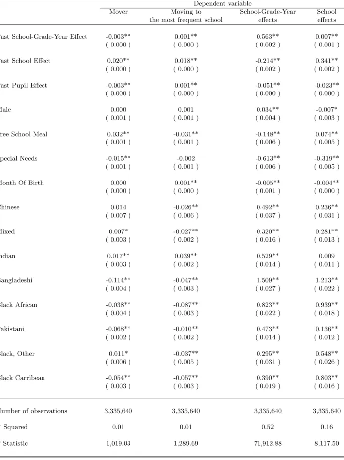
Table 10 offers an analysis of patterns of pupil mobility. At this stage, it does not aim at checking whether the identification assumptions required in our analysis are supported by the data. Rather, that analysis is deferred to the next section of the paper. Instead, at this juncture, we wish to provide some stylized facts about pupil mobility in English schools using the estimates of school and pupil effects.

The table shows two main patterns worthy of discussion. First of all, pupil mobility in primary school seems on the whole to be a feature of low performing pupils from low quality schools. Pupil effects are negatively correlated with next period school effects and school-grade-year effects. In-creasing the pupil effect by 10% of a standard deviation reduces the probability of moving by 0.3%. And increasing the pupil effect by 10% of a standard deviation is correlated with a 0.5 % fall of the next period school-grade-year and a 0.2% fall of the next period school effect. Free school meals are more likely to move (line 5 of table 10). They also move to particular schools, i.e. other schools than most pupils from their school. They move to lower quality school-grade-years (column 3). On the other hand, they move to schools with a higher school fixed effect. This means that they tend to go to schools with a worst peer group but better school quality.

The second main result is that disadvantaged ethnic backgrounds tend to move less than white children and movers from these ethnic backgrounds tend to go to better schools than white chil-dren. Bangladeshi pupils are 11.4% less likely to move than white chilchil-dren. Pakistani pupils are 6.8% less likely to move than white children and black caribbean children are 5.4% less likely to move. Bangladeshi especially tend to go to better schools, next period school-grade-year effects are higher by 15% of a standard deviation, school effects are higher by 12% of a standard deviation, conditionally on the school effect and school-grade-year effect of grade 2.

converges to aχ2 statistic (Hoel, 1962). 13

5

Robustness Checks and Further Discussion

In this section, we check present a number of robustness checks of our main finding, in particular focussing on whether our identification assumptions are supported by the data. The identification of school quality assumes at least sufficient mobility and exogenous mobility. The identification of peer effects moreover assumes that year-to-year variations in cohort composition are exogenous. We discuss these assumptions in the following subsections.

5.1 Do Children Move Enough to Generate Identification of the Model?

To separately identify pupil effects from school or school-grade-year effects, pupils have to move between schools. More precisely the mobility graph as defined in section 2.2 should have one connex component. Table 11 presents some basic statistics on mobility. Most pupils are followed from Key Stage 1 to Key Stage 2. A sizeable proportion (42%) of pupils also change school between grade 2 and grade 6. This is sufficient to generate only one mobility graph. The empirical question of importance of whether students who move are actually different from pupils who do not move is addressed in the following section.

5.2 Is Mobility Endogenous?

School quality and the effect of pupil background on achievement are estimated by comparing pupils’ test scores in different schools. It therefore requires that pupil mobility is not driven by unobserved shocks that affect test scores, such as divorce, unemployment, and other family events. We argue in this section that there is a credibly exogenous source of mobility. Indeed, some primary schools only cater for key stage 1 pupils. Mobility is compulsory in this case. It proves important that when the model is estimated on compulsory movers only, this paper’s results are not significantly affected.

i) Why Endogenous Mobility may be a Problem

We design a small, simple model to understand why endogenous mobility may be a problem. In this model, households experience unemployment shocks that are unobserved by the econometrician. When a household experiences an unemployment shock, children change school and their test scores are likely be lower.

The model is set up as follows. There are two periods. In each period, pupils’ parents can either be unemployedui,t = 1, or employedui,t = 0. Test scores are determined by the following equation:

yi,t = θi+ψJ(i,t)−δui,t+ηi,t (8)

(8) is a school effect model. We restrict ourselves to a model with school effects for expositional ease. yi,t is the test score of pupili in year t. ψj is the school effect of school j. δ is the adverse

effect of unemployment on test scores, and ui,t is a dummy for unemployment. ηi,t is a residual. Unemployment shocks ui,t, i= 1,2, t= 1,2, are unobserved and the econometrician estimates the following specification:

yi,t = ˆθi+ ˆψJ(i,t)+εi,t (9)

Assuming exogenous mobility, the estimated school effects ˆψj are estimated by OLS. To under-stand the relationship between the structural effects and the least squares estimates, let us write the specification in matrix form.

Y =Dθ+F ψ−δU +ε

withY the vector of test scores,D the design matrix for pupil effects,θ the vector of pupil effects,

F the design matrix for school effects,ψthe vector of school effects,U the vector of unemployment shocks and εthe residual.

The estimates are as follows:

ˆ

θ = θ−δ(D0MFD)−1D0MFU (10)

ˆ

ψ = ψ−δ(F0MDF)−1F0MDU (11)

where MD is the matrix that projects a vector on the vector space that is orthogonal to D. The same logic applies to MF.

Thus the estimates of the individual effects and the school effects are biased whenever the correlation between unemployment shocks and design matricesF orDis nonzero, that is, whenever mobility is endogenous. When unobserved unemployment shocks (i) drive pupils to particular schools and (ii) affect their test scores, the estimates of school effects and pupil effects are biased. ii) Compulsory Moves as an Exogenous Driving Force of Mobility

Compulsory movers are children who move between grade 2 and grade 6 because their key stage 1 school does not cater for key stage 2 children. This mobility is likely to be more exogenous than voluntary moves. However, there are three important conditions: (i) compulsory movers should not be significantly different from non compulsory movers; (ii) as compulsory mobility is expected by parents, we need to get evidence that key stage 1 only schools are not particular schools – either better or worse schools; (iii) compulsory mobility provides us with a exogenous reason to move, but it does not per se give an exogenous direction of mobility; children may still sort endogenously into schools.

Table 12 shows descriptive statistics for compulsory movers, noncompulsory movers and stayers. Genders, months of birth, languages and ethnicities are very similar between compulsory movers, noncompulsory movers and stayers. Differences between the three categories appear in the fraction

of special needs students and free school meals. The fraction of free school meal students is higher among noncompuslory movers than among compulsory movers, but it very similar between com-pulsory movers and stayers. On the whole, there are slight differences between the three categories of mobility.

We therefore performed the estimation of specifications SE and PSGYE on compulsory movers only14. Correlation tables (table 14) reveal that stylized facts are robust to the exclusion of noncom-pulsory movers: (i) pupil heterogeneity is bigger than school heterogeneity and school-grade-year heterogeneity (ii) the correlation between test scores and individual effects is bigger than the corre-lation between test scores and either school effects or school-grade-year effects.

Pupil heterogeneity is similar in table 4 and in table 14. School-grade-year or school hetero-geneity, while still smaller than pupil heterohetero-geneity, is bigger in the school effects specification with compulsory movers only (6.938 vs 1.941). This might be due to the smaller number of observa-tions in the estimation with compulsory movers only. School effects heterogeneity is comparable in the school-grade-year specification with and without noncompulsory movers. Stylized facts do not change when estimating regressions with compulsory movers only.

The last issue we need to address is whether the direction of mobility is likely to be an iden-tification issue. We define the most frequent school pupils go to. For each school j, the number of pupils who move from school j to school j0 is computed. The most frequent school pupils from school j go to in the next period is noted M(j). Among pupils who move, 63% move to the most frequent school (table 11). This is mainly made up of compulsory movers. Therefore compulsory movers mainly tend to go to the ’usual’ school, and the direction of their mobility is not likely to be mainly explained by individual unobserved time varying variables.

5.3 The Identification of Peer Effects: Are Year-to-Year Variations in Grade

Composition Exogenous?

The effect of grade composition on school quality is estimated by looking at how year-to-year variations affect school-grade-year effects. This actually requires that year-to-year variations in grade composition are not correlated with other changes in school inputs, such as changes in teacher quality and school funding. One way of addressing this identification issue is to compare year-to-year variations to truly random variations around school average composition.

Formally, if changes in grade composition are truly exogenous, they must be some random fluc-tuation around the average school composition. In a way identification relies on the idea that grade composition in a given year is a finite size approximation of the school’s equilibrium composition.

ˆ

E(z|j, g, t) =E(z|j, g) +uj,g,t (12)

Notations as before. ˆE(z|j, g, t) is the empirical school-grade-year composition in schoolj, gradeg

and yeart. This is a vector containing the percentage of each ethnicity, the percentage of boys, free

14

meals and special needs. E(z|j, g) is average school composition across the three cohorts. The size of the noise is approximately normal with variance aroundV ar E(z|j, g)/√nj,g,t.

The dataset only contains the empirical composition of grades. Therefore school average com-position is just an estimate of the true comcom-position.

ˆ

E(z|j, g) =E(z|j, g) +vj,g,t (13) with the size of the error term approximatelyV ar E(z|j, g)/√nj,g. Therefore, finally, ˆE(z|j, g, t) =

ˆ

E(z|j, g) +uj,g,t−vj,g,t.

Figure 2 compares the results of simulations to actual year-to-year variations in school-grade-year compositions. For boys, free meals and three important ethnic groups year-to-year variations are remarkably similar to random variations, as in Lavy and Schlosser (2007). This suggest that trends in school-grade-year composition are not likely to explain the results of peer effects regression. On the other hand, year-to-year varations in the fraction of special needs is bigger in the dataset than what would be expected if it were purely random. There may be trends in the fraction of special needs students in schools, which is likely to be due to evolving support for special needs students in English elementary schools. Broadly speaking, apart from special needs students, variations in gender and ethnic compositions are similar to random variations around average school composition.

5.4 What Can League Tables Tell Us?

The Education Reform Act 1988 set up the National Curriculum, which follows pupils through key stages, as we pointed out in section 3.1. Since the early 1990s league tables have been publicly available in England - for example, measures of performance at the end of each key stage are now disclosed on the BBC’s website and through local newspapers. This is a crucial element of transparency that is coupled with some leeway for school choice. Parents typically submit their first three choices to Local Education Authorities in the fall of the academic year before enrollment; most faith schools require a special application form.

Measures of performance are published in league tables. These league tables have become increasingly more sophisticated over time. They currently reveal three pieces of information: (i) the average test score at key stage examinations; (ii) the average value added of pupils in the school; value added is the difference between the pupil’s test score in the previous key stage and his current test score; finally, (iii) the average test score and value added in the local authority.

Are these elements informative about school effectiveness? The answer depends on the shape of the education production function. It turns out that, using our models, neither absolute test scores nor value added measures are good estimates of school effectiveness ϕ or ψ. In the full-fledged model with non-zero decay rate and past inputs, the average test score of a school is a mixture of school effectiveness, the average individual effect in the school and the average effectiveness of past schools. Indeed,

E[yi,f,t|j, g= 6, t] = (1 +λ)·E[θi|j, g= 6, t] +ϕj,g=6,t+λ·E[ϕj,g=2,t−4|j, g= 2, t−4] (14)

where notations are as before. t is the year, g = 6 says that we are considering test scores in grade 6. E[yi,f,2|j, g = 6, t] is the average test score in school j, grade g in grade 6. In two of the

three cohorts, the estimated decay rate is not different from zero. In this case, average past school effectiveness disappears but the average individual effect remains. Therefore, unless two schools have the same intake, the average test score is not informative about ϕ. Presumably this matters for issues of school accountability.

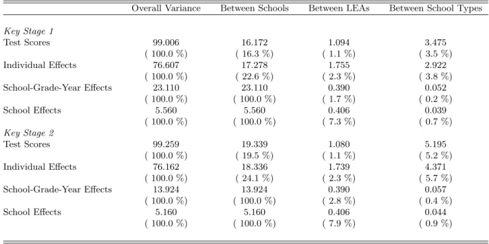
How important is the contribution of individual fixed effects to school average test scores? Table 15 shows the decomposition of the between-school variance of test scores into its components. Most of the variance of pupil effects is within schools (76%). There is however substantial between-school variance of the pupil effects (24% of the variance of pupil effects). More troubling, the between-school variance of individual effects is very close to the between-between-school variance of test scores. This suggests that average test scores are a flawed measure of school effectiveness, provided our specification is correct.

Value added measures are a means to get rid of these confounding effects. Average value added is:

E[∆yi,f|j, g= 6, t] =λ·E[θi|j, g= 6, t] +ϕj,g=6,t+ (λ−1)·E[ϕj,g=2,t−4|j, g= 2, t−4] (15)

where ∆yi,f = yi,f,2 −yi,f,1. E[∆yi,f|j, t] is average value added in school j, in a given year t. Again, λ is close to zero in most cohorts, so that average value added is free of the individual effects. However, average past school quality still enters the equation. It is a priori a problem since the variance of school effects in grade 2 is comparable to the variance of school effects in grade 6.

Overall, neither average test scores nor average value added measures are a good proxy for school effectiveness. It seems that more elaborate statistics are needed to truly help parents in accurately determining their school choice decisions. The findings of our paper suggest that an index which does not conflate pupil, school and peer effects and one that does not relate on value added could be superior. Of course, there is a trade-off between the complexity of our approach to generate measures and the ’simpler’ measures currently reported, but the estimates of school effects from our approach can be calibrated into the information set of those with an interest in which schools generate better performance for children.

Moreover, school effects are precisely estimated: the difference between the 60th percentile school effect and the 40th percentile school effect is significant in all specifications, with a standard error suggesting that our estimates could be used to differentiate school quality up to a percentile point.15 This is in stark contrast with Chay, McEwan and Urquiola (2005) and Bird, Cox, Farewell,

15

Goldstein, Holt and Smith (2005), which find that average test scores and value-added are essentially noisy measures.

5.5 Matching of Pupils to Schools

Results have shown that the most relevant specification is equation PSGYE. In this specification, schools are equally effective for all students, that is, there is no complementarity between pupils and schools. If the educational production function is truly specified as in specification PSGYE, the model does not predict any particular matching of pupil effects and school effects at equilibrium. Matching patterns are indeed determined by the complementarity between pupil effects and school effects, following Becker (1973)16. In such a world, the model predicts zero correlation between pupil effects and school-grade-year fixed effects.

However, some of the correlations between child effects and school effects in table 4 are negative. Does it mean that pupils with a high pupil effect are structurally matched with low school-grade-year effects? The correlation between estimated pupil effects and estimated school effects is actually downward biased and we perform simulations to estimate the magnitude of the bias, suggesting that the correlation is likely to be close to zero.

The correlation between estimated effects is downward biased. This has been pointed out in the context of worker-firm matched panel datasets (Abowd and Kramarz, 2004). To make this clear, let us decompose the correlation between child and school effects. This correlation can be written as the sum of the correlation between measurement errors and the true covariance between the effects.

Cov(ˆθ,ϕˆ) =Cov(ˆθ−θ,ϕˆ−ϕ) +Cov(ˆθ−θ, ϕ) +Cov( ˆϕ−ϕ, θ) +Cov(θ, ϕ)

whereθis the individual effect,ϕis the school-grade-year effect, ˆθis the estimated individual effect, ˆ

ϕis the estimated school-grade-year effect.

The estimation of Cov(θ, ϕ) therefore requires the estimation of Cov(ˆθ−θ, ϕ), Cov(ϕ,θˆ−θ),

Cov(ˆθ−θ,ϕˆ−ϕ). In general, the measurement errors of child and school effects are negatively correlated (Abowd and Kramarz, 2004). The intuition behind this result is that (i) pupils who change school get a better estimated effect but school effects are less precisely estimated (ii) pupils who do not change school have a less well estimated effect but their associated school effect is more precisely estimated.

Simulations can assess the order of magnitude of the downward bias of the correlation. We generate pupil effects who have a normal distribution with the same variance as the estimated pupil effects. We also generate school effects the same way. The point here is that pupil effects and school effects are uncorrelated. We then generate simulated test scores using the specification with past and current school-grade-year and individual effects.

used, with little difference on the size of standard errors. The differenceψP60−ψP40was 1.12 with a standard error of 0.057 in specification SGYE.

16_{This of course, assumes a particular form of preferences and special market conditions. The housing market should} be perfect, parents should know the educational production function as specified in equation PSGYE and the only reason for location decisions should be the level of test scores.