Similarity Based Reasoning Fuzzy
Systems and Universal Approximation
Sayantan Mandal and Balasubramaniam Jayaram
AbstractI
n this work, we show that fuzzy inference systems based on Similarity Based Reasoning (SBR) where the modification function is a fuzzy impli-cation is a universal approximator under suitable conditions on the other components of the fuzzy system.
Key words: Similarity Based Reasoning, Fuzzy implications, Universal ap-proximation.
1.1 Introduction
The termapproximate reasoning (AR) refers to methods and methodologies that enable reasoning with imprecise inputs to obtain meaningful outputs [?]. AR schemes involving fuzzy sets are one of the best known applications of fuzzy logic in the wider sense. Fuzzy Inference Systems (FIS) have many de-grees of freedom, viz., the underlying fuzzy partition of the input and output spaces, the fuzzy logic operations employed, the fuzzification and defuzzifi-cation mechanism used, etc. This freedom gives rise to a variety of FIS with differing capabilities. One of the important factors considered while employ-ing an FIS is its approximation capability. Many studies have appeared on this topic and due to space constraints, we only refer the readers to the following exceptional review on this topic [?] and the references therein.
In this work, we consider a Similarity Based Reasoning (SBR) FIS where similarity between the inputs and the antecedents is used to subsequently Department of Mathematics,
Indian Institute of Technology Hyderabad, Yeddumailaram-502205, INDIA
e-mail: ma10p002@iith.ac.in, jbala@iith.ac.in
modify the consequents to obtain a final output. Such inference schemes are also known as plausible reasoning scheme [?]. After detailing the inference mechanism in an SBR, we show that when the modification functions are modeled based on fuzzy implications, under suitable conditions on the other components of an SBR, the FIS based on SBR does become a universal approximator, i.e., can approximate a continuous function over a compact set to arbitrary accuracy. Also we deal only with single variable functions, alternately where the rule base consists of Single Input Single Output (SISO) rules.
1.2 Preliminaries
We assume that the reader is familiar with the classical results concerning fuzzy set theory and basic fuzzy logic connectives, but to make this work more self-contained, we introduce some notations, concepts and results employed in the rest of the work.
1.2.1 Fuzzy Sets
IfX is a non-empty set then we denote byF(X) the fuzzy power set ofX, i.e.,F(X) ={A|A:X →[0,1]}.
Definition 1.A fuzzy setAis said to be
• normal if there exists anx∈X such thatA(x) = 1,
• convexifXis a linear space and for anyλ∈[0,1],x, y∈X,A(λx+(1−λ)y)≥
min{A(x), A(y)}.
Definition 2.For anA∈ F(X), theSupport,Height,Kernel andCeiling of
A are denoted, respectively, as Supp A, HgtA, Ker A and CeilA and are defined as:
SuppA={x∈X|A(x)>0},
HgtA= sup{A(x)|x∈X} ,
KerA={x∈X|A(x) = 1},
CeilA={x∈X|A(x) = HgtA} .
Ais said to be bounded if Supp Ais a bounded set. Note that for a normal fuzzy set Ker A= CeilA.
We denote the space of fuzzy sets which are bounded, normal, convex and continuous asFBN CC(X). ClearlyFBN CC(X)⊆ F(X).
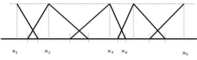
Fig. 1.1 An Illustrative Example for 13-type partition in Definition??
.
Definition 3.Let P be an arbitrary collection of fuzzy sets ofX, i.e,P =
{Ak}nk=1⊆ F(X).P is said to form afuzzy partition onX if
X ⊆
n
[
k=1
SuppAk .
In literature, a partitionP ofX as defined above is also called acomplete partition.
Definition 4.A fuzzy partitionP ={Ak}nk=1⊆ F(X) is said to be
• consistent ifAk(x) = 1 thenAj(x) = 0 for any j6=k.
• Ruspini partitionif
n
X
k=1
Ak(x) = 1 for everyx∈ X.
Definition 5.Let{xk}nk=1be a classical partition ofX, i.e.,X = n−2
[
k=1
[xk, xk+1)∪
[xn−1, xn]. IfP ={Ak}nk=1 be a fuzzy partition of the spaceX in such a way
that
• eachAk is normal atxk∈X, i.e.,Ak(xk) = 1,
• Supp Ak = xk−1+ xk−xk−1 3 , xk+1− xk+1−xk 3 for k = 2, . . . , n−1, while SuppA1=x1, x2−x2−3x1 and SuppAn = xn−1+xn−3xn−1, xn i , we call this type of partition as 1
3-type partition.
1.2.2 Defuzzification
Often there is a need to convert a fuzzy set to a crisp value, a process which is called Defuzzification. This process of defuzzification can be seen as a map-ping g : F(X) −→ X. There are many types of defuzzification techniques available in the literature, see [?] for a good overview. In this work, we use the following defuzzifier extensively.
Example 1.For an A∈ F(X), theFirst of Maxima (FOM) defuzzifier gives as output the smallest of all those values inX with the highest membership value, which can be mathematically expressed as
FOM(A) = min{x|A(x) = max
w A(w)}. (1.1)
Similarly theLast of Maxima (LOM) defuzzifier is defined as LOM(A) = max{x|A(x) = max
w A(w)}. (1.2)
1.2.3 Fuzzy Logic Connectives
Definition 6 ([?]). A binary operationT: [0,1]2→[0,1] is called at-norm,
if it is increasing in both variables, commutative, associative and has 1 as the neutral element.
Definition 7 ([?]).A functionI: [0,1]2→[0,1] is called afuzzy implication
if it is decreasing in the first variable, increasing in the second variable and
I(0,0) = 1,I(1,1) = 1,I(1,0) = 0. The set of all fuzzy implications will be denoted byI.
Definition 8 ([?]). A fuzzy implicationI: [0,1]2→[0,1] is said to
• satisfy the ordering property, if
I(x, y) = 1⇐⇒x≤y , x, y∈[0,1]. (OP)
• be a positive fuzzy implication ifI(x, y)>0, for allx, y∈(0,1).
1.3 Fuzzy Inference Mechanism
Given two non-empty classical sets X, Y ( R, a fuzzy Single Input Single
Output (SISO) IF-THEN rule is of the form:
where ˜x, ˜y are the linguistic variables and A ∈ F(X), B ∈ F(Y) are the linguistic values taken by the linguistic variables. A knowledge base consists of a collection of such rules. Hence, we consider a rule base ofn SISO rules which is of the form:
IFx˜is Ai THENy˜isBi , (1.4)
where ˜x, ˜yandAi ∈ F(X), Bi∈ F(Y), i= 1,2, . . . nare as mentioned above.
As an example, consider the rule
IFTemperature isHigh THENFanspeed isMedium.
HereTemperatureandFanspeed are the linguistic variables andHigh,Medium
are the linguistic values taken by the linguistic variables in a suitable domain. Now given a single SISO rule (??) or a rule base (??) and given any input ” ˜x
isA0” , the main objective of an inference mechanism is to findB0 such that ” ˜y is B0 ”. Many types of inference mechanisms are available to us in [?],
[?], [?], etc. Here we consider only the case of Similarity Based Reasoning.
1.4 Similarity Based Reasoning (SBR)
Consider the fuzzy if-then rule (??). Let the given input be ˜xisA0. Inference in Similarity Based Reasoning (SBR) schemes in AR is based on the calcu-lation of a measure of compatibility or similarity M(A, A0) of the input A0
to the antecedent Aof the rule, and the use of a modification functionJ to modify the consequent B, according to the value ofM(A, A0).
Some of the well known examples of SBR are Compatibility Modification Inference (CMI) [?], ”Approximate Analogical Reasoning Scheme” (AARS) in [?] and ”Consequent Dilation Rule” (CDR) in [?], Smets and Magrez [?], Chen [?], etc. In this section, we detail the typical inferencing mechanism in SBR, but only in the case of SISO fuzzy rule bases.
1.4.1 Matching function M
Given two fuzzy sets, say A, A0, on the same domain, a matching function
M compares them to get a degree of similarity, which is expressed as a real in the [0,1] interval. We refer toM as the Matching Function in the sequel. Formally,M :F(X)× F(X)→[0,1].
Example 2.LetXbe a non-empty set andA, A0∈ F(X). Below we list a few of the matching functions employed in the literature.
• Zadeh [?]: MZ(A, A0) = max
x∈Xmin(A(x), A
• Magrez - Smets [?]: Given a fuzzy negationN,
MM(A, A0) = max
x∈Xmin(N(A(x)), A
0(x)).
• Measure of Subsethood [?]: For anI∈ F I,
MS(A, A0) = min
x∈XI(A
0(x), A(x)).
Definition 9.Let F∗ ⊆ F(X) be an arbitrary collection (not necessarily a
fuzzy partition) of fuzzy sets on X. M is said to be consistent with F∗ if
for anyA∈ F∗,
M(A, A) = 1. (MCF)
Definition 10.LetP = {Ak}nk=1 ⊆ F
∗ be the given fuzzy partition of X.
LetA0∈ F∗.M is said to beconsistent with P (andF∗) if
n
X
k=1
M(A0, Ak)≤1. (MCP)
Definition 11.The matching functionM is said to be Strongif
KerA⊆KerB or Ker B⊆KerA=⇒M(A, B) = 1 (MS)
Example 3.Let X ( R be any bounded interval andF∗=F
BN CC(X). For
a given fuzzy partition P = {Ak}nk=1 ⊆ FBN CC(X) , we define a maching
function as, MP(Ak, A0) = Area(A0∩Ak) Area(A0) , A 0∈ F BN CC(X). (1.5)
ClearlyM satisfies (??), (??) and (??).
Example 4.Let X ( R be any bounded interval. Let the antecedent fuzzy
sets{Ak}nk=1=PX ⊆ F∗(X) partition the input spaceX such that it forms
a partition of the type defined in Definition??.
Now, if x0 ∈ X is the input letA0 ∈ F(X) be the fuzzified input such thatA0 attains normality atx0, i.e.,A0(x0) = 1. Then the matching function defined asM(A0, A) =A(x0) for anyA∈ F(X) has the property (??).
1.4.2 Modification Function
J
Let A0 be the fuzzy input and s = M(A, A0) ∈ [0,1], a measure of the compatibility ofA0 toA.
The modification function J is again a function from [0,1]2 to [0,1] and, given the rule (??), modifies B ∈ F(Y) to B0 ∈ F(Y) based on s, i.e., the
consequent in SBR, using the modification functionJ, is given by
B0(y) =J(s, B(y)) =J(M(A, A0), B(y)), y∈Y.
In AARS [?] the following modification operators have been used: (i) JML(s, B) =B0(x) = min{1, B(x)/s} , x∈X;
(ii) JMVR(s, B) =B0(x) =s·B(x), x∈X.
In CMI [?] and CDR [?] J is taken to be a fuzzy implication operator. In fact,JML(s, B) =IGG(s, B), whereIGG is the Goguen implication [?].
1.4.3 Aggregation Function
G
In the case of multiple rules
Ri: IF ˜xisAi THEN ˜yisBi, i= 1,2, . . . , m,
we infer the final output by aggregating over the rules, using an associative operatorG: [0,1]2→[0,1] as follows: B0(y) =Gmi=1 J M(Ai, A0), Bi(y) , y∈Y. (1.6)
Usually,Gis at-norm,t-conorm or a uninorm [?].
1.5 Fuzzy Systems
F
based on SBR
An SBR fuzzy inference system can be represented by the hexatuple F =
{R(Ai, Bj), f, M, J, G, g} where
• Ris the fuzzy if-then rule base formed from the fuzzy partitions{Ai},{Bj}
onX, Y, respectively,
• f :X −→ F(X) is called the fuzzification mapping that maps an element
x∈X to a fuzzy set ofF(X),
• M is matching function,
• J is modification function,
• Gis aggregation function, and
• g:F(Y)→Y is any defuzzifier, that converts the output fuzzy set to a crisp valuey∈Y.
We considerFwith the following assumptions on the different components /
1.5.1 The Fuzzy Partitions
A
i, B
jLet X, Y ( R be arbitrary but fixed and let F∗(Z) = F
BN CC(Z), where
Z =X orY.
Let the antecedent fuzzy sets{Ak}nk=1=PX ⊆ F∗(X) partition the input
space X such that it forms a partition of the type defined in Definition??, which also implies it is complete.
Similarly, let the consequent fuzzy sets {Bj}mj=1 = PY ⊆ F∗(Y) form a
complete and Ruspini partition of the output spaceY.
1.5.2 The Fuzzified Input
A
0Let us consider a fuzzificationf :X −→ F∗(X) that mapsx0 ∈X to a fuzzy
set ofA0∈ F∗(X) =F
BN CC(X) such that
Supp (f(x0) =A0)∩SuppAk6=∅,
for someAk ∈ PX. Moreover it is assumed thatA0 intersects only two of the
adjacent fuzzy setsAk i.e, SuppA0∩ SuppAk 6=∅if and only ifk=m, m+1
for somem∈Nn−1.
Note that it is with this fuzzified input A0 the antecedentsAi of the
dif-ferent rules are matched against.
Example 5.Let {xk}nk=1 be a crisp partition ofX. Let{Ak}nk=1 partitioning
the input spaceX be such thatAk ∈ PX and forms a fuzzy partition of the
type defined in Definition??. Then if we take
| SuppA0| ≤ 1 3 · l min i=1 n |xi+1−xi| o ,
thenA0 intersects atmost two of the adjacent fuzzy setsAk.
1.5.3 The Operations
M, J, G
We choose a matching function M such that M is Consistent w.r.to the partitionPX given in Section??, i.eM satisfies both (??) and (??).
We choose the modification function J to be a fuzzy implication, i.e.,
J ∈ F I. For notational convenience we will denote it by ” −→ ” in the sequel.
1.5.4 The Fuzzy Output
B
0With the above assumptions, the output fuzzy setB0 for a given crisp input
x0 (or fuzzy inputA0) takes the form as given in the following lemma: Lemma 1.With the operations of of the SBR FIS (??)as in Sections??
-?? the fuzzy output of the SBR FIS (??), for a given inputx0 ∈X is given by
B0(y) =T[sm−→Bm(y), sm+1−→Bm+1(y)] , (1.7) wheresm=M(A0, Am)andsm+1=M(A0, Am+1).
Proof. With the above operationsM, J, Gthe fuzzy output for a given input
x0∈X is given by (??) as follows: B0(y) =T M(A0, A1)−→B1(y)), M(A0, A2)−→B2(y), . . . , . . . , M(A0, An)−→Bn(y) .
We can write the above as
B0(y) =Tkn=1[M(A0, Ak)−→Bk(y)]. (1.8)
By the choice of our fuzzification based on our above notations on A0, Ak,
viz., that A0 intersects only two adjacent fuzzy sets among the {Ak}, say
Am, Am+1, we have thatM(A0, Ak) = 0 for allk6=m, m+ 1. Note also that
I(0, y) = 0−→y= 1 for anyy∈[0,1]. Now, the fuzzy outputB0(y) for any
y∈Y which is given by (??) becomes
B0(y) =Tkn=1[M(A0, Ak)−→Bk(y)], =ThTk6=m,m+1 M(A0, Ak)−→Bk(y) , M(A0, Am)−→Bm(y), M(A0, Am+1)−→Bm+1(y) i =ThM(A0, Am)−→Bm(y), M(A0, Am+1)−→Bm+1(y) i =T[sm−→Bm(y), sm+1−→Bm+1(y)] = (??).
1.5.5 The Defuzzified Output
g
(
x
0)
We have chosen the modification function J to be a fuzzy implication, i.e.,
J =I∈ F I. Assuming that the considered modification functionJ has (??), we define the defuzzification functiongappropriately so thatgis continuous. In the following, we discuss the explicit formulae for g. Note thatg is also known as the system function of the fuzzy systemF[?], [?].
1.6 SBR Fuzzy Systems and Universal Approximation
In this section, we show thatF={R(Ai, Bi), M, J, G, g}such that the fuzzypartitions {Ak},{Bk} and the operations M, J, G, g as given in Sections??
-?? are universal approximators, i.e., they can approximate any continuous function over a compact set to arbitrary accuracy.
Theorem 1.For any continuous function h: [a, b] → R over a closed
in-terval and an arbitrary given > 0, there is an SBR fuzzy system F =
{R(Ai, Bi), M, J, G, g} withM having the property (??) w.r.to PX ={Ai},
J having (??), G being a t-norm and g as given in (??) or (??) such that
max
x∈[a,b]
|h(x)−g(x)|< .
Proof. We prove this result in the following steps. Step I : Choosing the points of normality
Sincehis coninuous over a closed interval [a, b],his uniformly continuous on [a, b]. Thus for a given >0 there existsδ >0 such that
|w−w0|< δ=⇒ |h(w)−h(w0)|<
2 .
Step I (a): A Coarse Initial Partition
With the δ = δ() defined above and taking l = b−a δ
we now choose
wi∈X, i= 1,2, . . . l, such that|wi−wi+1|< δ.
Letzi =h(wi), the valuehtakes at the above chosenwi, fori= 1,2, . . . l.
We call these pointswiandzi the points of normality on the input space and
the output space respectively.
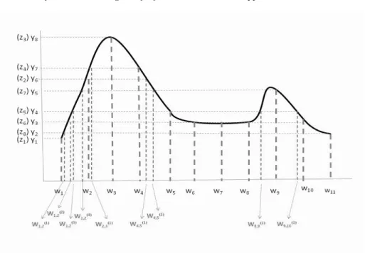
In Fig. ??, the pointsw1, w2, . . . , w11 and the points z1, z2, . . . z8 are the points of normality in the input and the output spaces, respectively.
Step I (b): Redundancy Removal and Reordering
Let us choose the distinctzi’s from the above and sort them in ascending
order. Letσ :Nl −→Nk denote the above permuation map such that zi =
uσ(i), fori= 1,2, . . . landuj, j= 1,2, . . . , k are in ascending order.
By rearranging the zi’s in ascending order and renaming them we have obtained: u1 =z1, u2 =z8, u3=z6, u4 =z5, u5 =z7, u6=z2, u7 =z4, u8 =
z3.
Step I (c): Refinement of the input space partition:
Thus for each i = 1,2, . . . , l we have h(wi) = zi = uσ(i). However, note
that consecutive points of normalitywi, wi+1 in the input space need not be
mapped to consecutive points of normalityuσ(i), uσ(i)+1or uσ(i), uσ(i)−1. In Fig.??,h(w1) =u1 andh(w2) =u6. Thus for the consecutive points
w1 andw2 the function values areu1 andu6, which are not consecutive.
To ensure the above, we further refine the input space partition. To this end, we refine every sub-interval [wi, wi+1], for i = 1,2, . . . l−1 as follows.
Note thath(wi+1) =uσ(i+1).
Fig. 1.2 An Illustrative Example forStep Iin the proof of Theorem??.
For everyi= 1,2, . . . l−1 do the following: (i) Ifuσ(i+1)=uσ(i)+1 oruσ(i)−1then we do nothing.
(ii) Let uσ(i+1) = uσ(i)+p, where p ≥ 2. For every u ∈ {uσ(i)+1, uσ(i)+2, . . . ,
uσ(i)+p−1} we find a pointv ∈[wi, wi+1] such thath(v) =u. Note that the
existence of such av∈[wi, wi+1] is guaranteed by the continuity - essentially
the ontoness - of the functionh. Ifu=uσ(i)+q, for some 1≤q≤p−1, then
we denote the pointv asw(i,iq)+1.
(iii) Similarly, let uσ(i+1) = uσ(i)−p, where p ≥ 2. For every u ∈ {uσ(i)−1,
uσ(i)−2, . . . , uσ(i)−p+1} we find a v ∈ [wi, wi+1] such that h(v) = u. Once
again, ifu=uσ(i)−q, for some 1≤q≤p−1, then we denotev asw (q) i,i+1. From Fig. ??, it can be seen that we have inserted points w1
1,2, w21,2, w13,2,
w4
1,2 ∈ [w1, w2]. Proceeding similarly, the following sub-intervals, shown in Fig.??, have been refined:[w2, w3],[w4, w5],[w8, w9]and[w9, w10].
Step I (d): Final Points of Normality:
Once the above process is done, we again rename the points of normality
w(i,iq)+1 in the input spaceX in ascending order asx1, x2, . . . , xn(n≥l) and
theuσ(i)’s of the the output space asy1, y2, . . . yk.
Step II : Construction of the Fuzzy Partitions
In the next step, we construct fuzzy sets on both the input and output spaces with the above obtained xi’s and yj’s as the points of normality, as
Step II(a): Fuzzy Partition on the input space We constructlfuzzy sets such that • eachAi is centered atxi, • SuppAi= xi−1+ xi−xi−1 3 , xi+1− xi+1−xi 3
fori= 2, . . . , l−1, while Supp
A1 = x1, x2−x2−3x1 and SuppAl= xl−1+ xl−xl−1 3 , xl i ,
• eachAi is normal atxi, i.e., Ai(xi) = 1,
• eachAi is a continuous convex fuzzy set,
• {Ai}li=1form a partition as defined in Definition??.
For instance, if each of the Ai’s (i = 2, . . . , l−1) is a triangular fuzzy set andA1, Al are half-triangular with all of them attaining normality atxi then clearly we can construct {Ai}li=1’s partitioning the input spaceX as in Def-inition ??and are continuous, convex, of finite support andAi(xi) = 1.
Step II(b): Fuzzy Partition on the output space
Now we have the output space partition points asy1, y2, . . . yk. We
parti-tion the output space such that B1, B2, . . . Bk form a Ruspini partition (as
above) withBj(yj) = 1, j= 1,2, . . . k.Here obviously,
|yj−yj−1|<
2, j= 1,2, . . . k.
Further, let the fuzzy sets {Bj}kj=1 be continuous, convex and of finite
support along the same lines as theAi’s above, i.e., SuppB1= [y1, y2), Supp
Bj = (yj−1, yj+1), j= 2,3, . . . k−1, SuppBk = (yk−1, yk].
Step III: Construction of thesmooth rule base We construct the rule base with lrules of the following form:
IFxisAi THENy isBi, i= 1,2, . . . l, (1.9)
where the consequentBiin thei-th rule is chosen such thati=jis the index
of that yj=h(xi), wherexi is the point at whichAi attains normality.
Note that, since h is continuous, by the above assignment of the rules, we have that rules whose antecedents are adjacent also have adjacent conse-quents, i.e., for anyi= 1,2, . . . l−1 we have SuppBi∩SuppBi+16=∅. Thus
the constructed rule base is smooth as defined in [?]. Step IV : Approximation capability of the output
Now we consider an SBR fuzzy system with Multiple SISO rules of the form (??). Letx0 ∈X be the given input. Clearly,x0 ∈[xm, xm+1] for some
m∈Nl. Now as in section??, we fuzzifyx0 in such a way that the fuzzified
inputA0 (withA0(x0) = 1) intersects atmost two of theAi’s, say,Am, Am+1. For instance, one could take A0 as in Example??.
B0(y) =T M(A0, Am)−→Bm(y), M(A0, Am+1)−→Bm+1(y) =Tsm−→Bm(y), sm+1−→Bm+1(y) ,
where sm = M(A0, Am) and sm+1 = M(A0, Am+1). Note that by our
as-sumption on M, we have thatsm+sm+1≤1.
The output fuzzy set B0 is given by (??). We consider the kernel of B0, i.e., KerB0={y:B0(y) = 1}. We choose the defuzzified outputy0 such that it belongs to KerB0.
Since T is a t-norm, we know that T(p, q) = 1 if and only ifp = 1 and
q= 1. Noting thatJ has (OP), i.e.,p−→q= 1⇔p≤qandsm+sm+1≤1,
we have KerB0 ={y:B0(y) = 1} ={y:sm−→Bm(y) = 1} \ {y:sm+1−→Bm+1(y) = 1} ={y:sm≤Bm(y)} \ {y:sm+1≤Bm+1(y)}.
Letαm= min{α:sm−→α= 1} and βm+1 = min{β:sm+1−→β = 1}.
SinceJ has (OP), clearlyαm=smandβm+1=sm+1.
By the continuity and convexity ofBm, Bm+1there existam, bm,am+1, bm+1
such that Bm(am) = Bm(bm) = sm and Bm+1(am+1) = Bm+1(bM=1) =
sm+1. By the monotonicity of the implication in the second variable, for every
y ∈[am, bm] we have thatsm →Bm(y) = 1 and for every y ∈[am+1, bm+1]
we have thatsm+1→Bm+1(y) = 1. Thus,
{y:sm≤Bm(y)}= [am, bm], and {y:sm+1≤Bm+1(y)}= [am+1, bm+1]. Hence, KerB0={y:B0(y) = 1}= [am, bm] \ [am+1, bm+1]. (1.10) Claim: KerB0= [a m+1, bm]6=∅.
Firstly, note that for anysm∈[0,1] by the normality ofBmwe have that
Bm(ym) = 1 and hence ym ∈ {y : sm ≤ Bm(y)} = ym ∈ [am, bm] 6= ∅.
Similarly, ym+1∈[am+1, bm+1]6=∅. it suffices to show thatam+1≤bmfrom
whence Ker B0= [am+1, bm].
Note that since m < m+ 1, ym < ym+1 and from am+1 ∈ SuppBm+1
we have that ym ≤ am+1 ≤ ym+1. Similarly, ym ≤ bm ≤ ym+1. Hence,
ym≤am+1, bm≤ym+1.
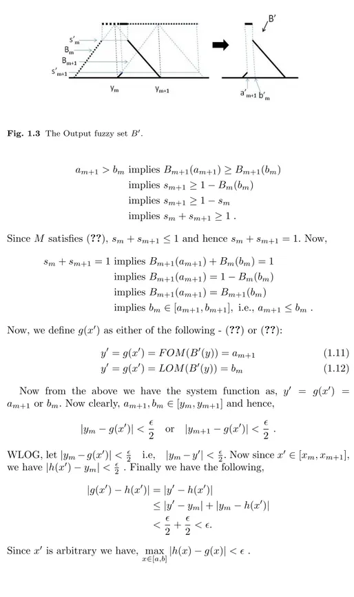
Fig. 1.3 The Output fuzzy setB0.
am+1> bm impliesBm+1(am+1)≥Bm+1(bm)
impliessm+1≥1−Bm(bm)
impliessm+1≥1−sm
impliessm+sm+1≥1.
SinceM satisfies (??),sm+sm+1≤1 and hencesm+sm+1= 1. Now,
sm+sm+1= 1 impliesBm+1(am+1) +Bm(bm) = 1
impliesBm+1(am+1) = 1−Bm(bm)
impliesBm+1(am+1) =Bm+1(bm)
impliesbm∈[am+1, bm+1], i.e.,am+1≤bm.
Now, we define g(x0) as either of the following - (??) or (??):
y0=g(x0) =F OM(B0(y)) =am+1 (1.11)
y0=g(x0) =LOM(B0(y)) =bm (1.12)
Now from the above we have the system function as, y0 = g(x0) = am+1 orbm.Now clearly,am+1, bm∈[ym, ym+1] and hence,
|ym−g(x0)|<
2 or |ym+1−g(x
0)|<
2 .
WLOG, let|ym−g(x0)|< 2 i.e, |ym−y0|< 2.Now sincex0 ∈[xm, xm+1],
we have |h(x0)−ym|< 2 .Finally we have the following,
|g(x0)−h(x0)|=|y0−h(x0)| ≤ |y0−y m|+|ym−h(x0)| < 2+ 2 < . Sincex0 is arbitrary we have, max
Remark 1.Note that withg as in (??) or (??) and sinceM satisfies (??), if
x0=xk ∈X we haveM(A0, Ak) = 1 and we obtainB0 =Bk, i.e.,g(x0) =yk
and the interpolativity of the inference is preserved.
References
1. D. Driankov, H. Hellendoorn, M. Reinfrank, An introduction to fuzzy control (2nd ed.), Springer-Verlag, London, UK, UK, 1996.
2. D. Tikk, L. T. K´oczy, T. D. Gedeon, A survey on universal approximation and its limits in soft computing techniques, Int. J. Approx. Reasoning 33 (2) (2003) 185–202. 3. D. Dubois, H. Prade, The generalized modus ponens under sup-min composition: a the-oretical study, in: Approximate Reasoning in Expert Systems, Elsevier/North-Holland. 4. S. Roychowdhury, W. Pedrycz, A survey of defuzzification strategies, International
Journal of Intelligent Systems 16 (6) (2001) 679–695.
5. E. P. Klement, R. Mesiar, E. Pap, Triangular Norms, Vol. 8 of Trends in Logic, Kluwer Academic Publishers, Dordrecht, 2000.
6. M. Baczy´nski, B. Jayaram, Fuzzy Implications, Vol. 231 of Studies in Fuzziness and Soft Computing, Springer, 2008.
7. W. Bandler, L. J. Kohout, Semantics of implication operators and fuzzy relational products, International Journal of Man-Machine Studies 12 (1) (1980) 89 – 116. 8. L. A. Zadeh, Outline of a new approach to the analysis of complex systems and decision
processes, IEEE Transactions on Systems, Man and Cybernetics.
9. P. Magrez, P. Smets, Fuzzy modus ponens: A new model suitable for appli-cations in knowledge-based systems, Int. J. Intell. Syst. 4 (2) (1989) 181–200. doi:10.1002/int.4550040205.
10. V. Cross, T. Sudkamp, Fuzzy implication and compatibility modification, in: Fuzzy Systems, 1993., Second IEEE International Conference on, 1993, pp. 219–224 vol.1. 11. I. Turksen, Z. Zhong, An approximate analogical reasoning approach based on
simi-larity measures, IEEE Transactions on Systems, Man and Cybernetics.
12. N. N. Morsi, A. A. Fahmy, On generalized modus ponens with multiple rules and a residuated implication, Fuzzy Sets and Systems 129 (2) (2002) 267 – 274.
13. S.-M. Chen, A new approach to handling fuzzy decision-making problems, in: Multiple-Valued Logic, 1988., Proceedings of the Eighteenth International Symposium on, 1988. 14. L. A. Zadeh, The concept of a linguistic variable and its application to approximate
reasoning-III, Information Sciences 9 (1975) 43–80.
15. Y.-M. Li, Z.-K. Shi, Z.-H. Li, Approximation theory of fuzzy systems based upon genuine many-valued implications: SISO cases, Fuzzy Sets Syst. 130 (2002) 147–157. 16. Y.-M. Li, Z.-K. Shi, Z.-H. Li, Approximation theory of fuzzy systems based upon
genuine many-valued implications: MIMO cases, Fuzzy Sets Syst. 130 (2002) 159–174. 17. M. ˇStˇepniˇcka, B. D. Baets, Monotonicity of implicative fuzzy models, in: FUZZ-IEEE 2010, IEEE International Conference on Fuzzy Systems, Barcelona, Spain, 18-23 July, 2010, Proceedings, 2010, pp. 1–7.