Big Data Optimization in Machine Learning

(1)

Lehigh University

Lehigh Preserve

Theses and Dissertations

2016

Big Data Optimization in Machine Learning

Xiaocheng Tang

Lehigh University

Follow this and additional works at:http://preserve.lehigh.edu/etd Part of theIndustrial Engineering Commons

Recommended Citation

Tang, Xiaocheng, "Big Data Optimization in Machine Learning" (2016).Theses and Dissertations. 2837.

(2)

Big Data Optimization in Machine Learning

by

Xiaocheng Tang

A Dissertation

Presented to the Graduate Committee of Lehigh University

in Candidacy for the Degree of Doctor of Philosophy

in

Industrial Engineering

Randomized Derivative-Free Optimization

of Noisy Functions

by

Ruobing Chen

Presented to the Graduate and Research Committee of Lehigh University

in Candidacy for the Degree of Doctor of Philosophy

in

Industrial and Systems Engineering

Lehigh University January 20, 2015

Lehigh University January, 2016

(3)

(4)

Approval of the Doctoral Committee

Big Data Optimization in Machine Learning

Xiaocheng Tang

Approved and recommended for acceptance as a dissertation in partial fulfillment of the requirements for the degree of Doctor of Philosophy.

Date

Dissertation Advisor

Committee Members:

Dr. Katya Scheinberg, Committee Chair

Dr. Frank E. Curtis, Dissertation Advisor

Dr. Nader Motee, Dissertation Advisor

(5)

Dedication

(6)

Acknowledgments

First and foremost, I would like to express my greatest appreciation to my advisor and dissertation committee chair Dr. Katya Scheinberg who has provided me guidance and support ever since the beginning of my Ph.D. study. She is an amazing advisor and has always inspired me to reach for a higher level.

I would like to thank my committee members, Dr. Frank E. Curtis, Dr. Nader Motee and Dr. Jorge Nocedal. Their insightful comments and constructive advices have been invaluable. Without their guidance and persistent help, this dissertation would not have been possible.

I also wish to thank Peiyan who has been hugely supportive throughout the several years it has taken to finish this work.

And finally I would like to thank all my friends, professors and faculties at Lehigh, and everyone else who has helped me complete this dissertation. Without their con-tinued efforts and support, I would have not been able to bring my work to a successful completion.

(7)

List of Tables

2.1 Per Iteration Complexity . . . 25

3.1 Datasets statistics used in experiments. Dataset itp and ads have the same exact dimension, but are constructed differently – itp tar-gets users’ general interest and includes users’ activities from other category-related events besides ads view or ads click. . . 67

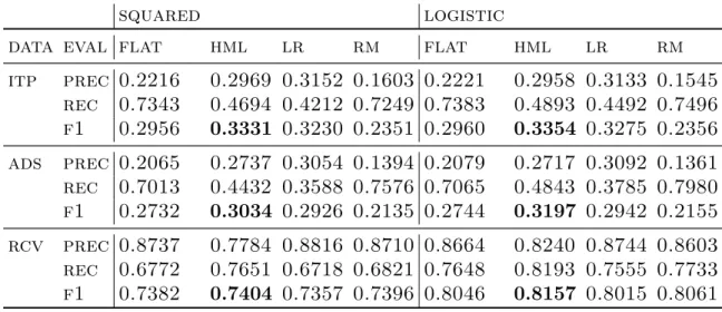
3.2 The comparison of FLAT, HML, Leaf Reduce (LR) and Root Map (RM) on all three datasets, with squared and logistic loss function, and evaluated by precision, recall and f1 score. . . 67

5.1 Row and column operations on LMatrix type M ∈ _Rn×m_{. Note that} while one memcpy ormemmoveon O(n) data has a complexity ofO(n), the constant in front of n can be much smaller than 1 (hence much faster than normaln flops), due to the use of cache optimizations and specialized processor instructions such as SIMD in those built-in library functions. . . 112

5.2 Data sets used in the experiments. . . 123

5.3 Compare the performance of different active-set strategies. . . 127

(11)

List of Figures

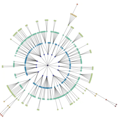
1.1 Visualization of taxonomy among labels in datasetads. . . 6

2.1 The hierarchy tree of the labels. . . 29

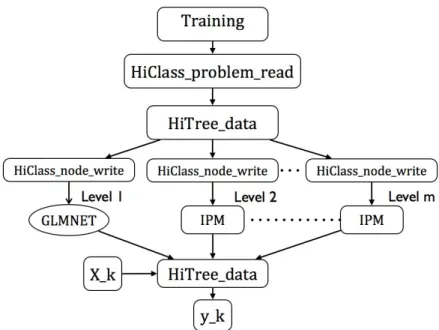
2.2 HiClass system flow chart . . . 32

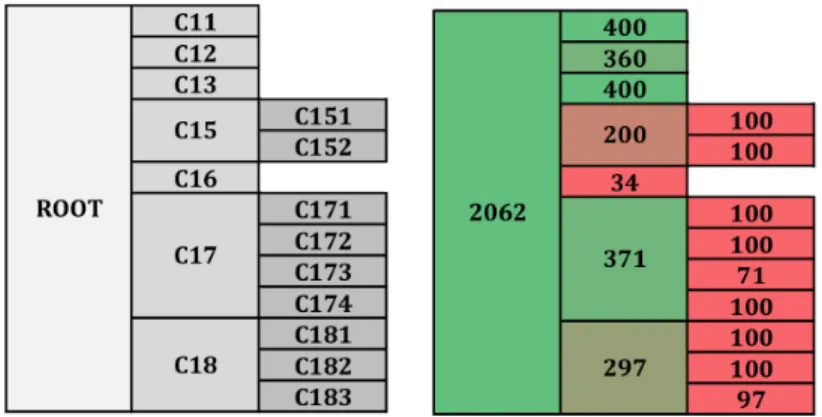
2.3 CCAT subtree . . . 34

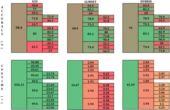
2.4 Performance comparison at each node between above mentioned algo-rithms. For HYBRID, we use GLMNET in the upper level and IPM at bottom. The number in the leftmost block of each table denotes the corresponding performance measure on the whole tree. For exam-ple, as shown by the rightmost upper table, 70% aggregate accuracy is achieved using the novel HYBRID method. . . 36

2.5 MCAT subtree . . . 37

2.6 Performance comparison at each node between above mentioned algo-rithms. . . 38

2.7 Illustration of Load Series Periodicity. . . 41

3.1 The tree structure is illustrated with blue rectangles as nodes and straight lines as edges. Groupsg are green translucent rectangles cov-ering nodes that are contained in the group. . . 61

(12)

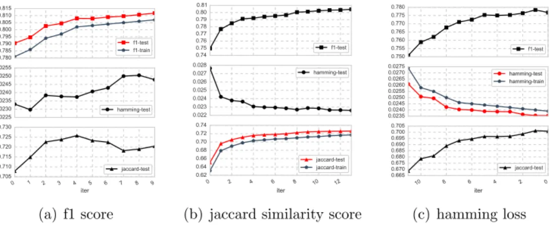
3.2 Testing and training performance under different metrics as learning objective on rcv dataset. Take (b) for example. HML equipped with jaccard similarity as the learning objective is applied on a training set of 3000 instances. Solutions after each iteration (the x-axis) of HML are recorded and later evaluated under all three metrics on the fullrcv

dataset (test set). The red curve denotes the objective values evaluated on the test set. In the same subplot along with the red curve are the objective values evaluated at different iterations on the training set. Other two subplots illustrate the same solutions evaluated by other

two metrics on the same test set. . . 68

5.1 Illustrate the dynamics of the four index sets (5.4.1) as x→x∗. Note how |Z1(x)| and |Z2(x)| start from the top and the bottom, respec-tively, and come together in the end, each containing (roughly) half the size of non-zero elements inx∗. Also note that |Z3(x)| vanishes at optimality. . . 126

5.2 Evolution of free sets in STD and GRDY-AD. Left: dataset mnist (p = 784, N = 1,000,000). Right: dataset gisette (p = 5000, N = 6000). The line plots are the size of free set against iterations and the bars denote the total sum of free set sizes over all iterations . . . 126

5.3 Study different inner loop termination criteria and its effect on algo-rithm performance. Time (top) and iterations (bottom) comparison for different l(k): log, linear, constant 5 and constant 200. . . 128

5.4 Consider linear functionl(k) = ak+b and study the effect ofaon run-ning time and iterations for different inner algorithm, i.e., coordinate descent (a) and proximal gradient (b). . . 129

5.5 Convergence plots on SICS (the y-axes on log scale). . . 135

5.6 RCD step count of LHAC on different SICS data sets. . . 136

5.7 Convergence plots on SLR (the y-axes on log scale). . . 137

(13)

Abstract

Modern machine learning practices at the interface of big data, distributed envi-ronment and complex learning objectives post great challenges to designing scalable optimization algorithms with theoretical guarantees. This thesis, built on the recent advances in randomized algorithms, concerns development of such methods in practice and the analysis of their theoretical implications in the context of large-scale struc-tured learning problems, such as regularized regression/classification, matrix com-pletion, hierarchical multi-label learning, etc. The first contribution of this work is thus a hybrid hierarchical learning system that achieve efficiency in a data-intensive environment. The intelligent decoding scheme inside the system further enhances the learning capacity by enabling a rich taxonomy representation to be induced in the label space. Important factors affecting the system scalability are studied and further generalized. This leads to the next contribution of the work – a globally con-vergent inexact proximal quasi-Newton framework and the novel global convergence rate analysis. This work constitutes the first global convergence rate result for an algorithm that uses randomized coordinate descent to inexactly optimize subprob-lems at each iteration. The analysis quantifies precisely the complexity structure of proximal Newton-type algorithms, which makes it possible to optimize based on that structure to reduce complexity. The final contribution of the work is a practical algo-rithm which enjoys global convergence guarantee from the framework. The algoalgo-rithm is memory- and communication-efficient and directly addresses the big data learning cases when both N (samples) and n (features) are large. We demonstrated that this general algorithm is very effective in practice and is competitive with state-of-the-art

(14)

(15)

Chapter 1

Introduction

The basic problem of interest in this work is the unconstrained minimization given by:

min

x∈_RnF(x)≡f(x) +g(x) (1.0.1) where f, g : _Rn _→

R are both convex functions such that f is twice differentiable,

with a bounded Hessian, andg is Lipschitz continuous, often non-smooth and in many applications has the following separable structure

g(x) =

J X

j=1

λjgj(xj) (1.0.2)

where each gj is a convex function; λ > 0 is a parameter; and xj ∈ Rnj denotes a

partition of the component ofx, e.g., the widely-used`1 regularization is obtained by

choosing gj =| · |, nj = 1,∀j.

Also known as composite optimization, problems of the form (1.0.1) have been the focus of much research lately at the interface of optimization and machine learn-ing. This form encompasses a variety of machine learning models, in which feature selection or structured learning is desired, e.g.,

• regularized logistic regression, where f computes the logistic loss on the given training set and the regularizerg can be group-`1/`2 depending on the problem.

(16)

• inverse covariance estimation, where f(X) = −log detX + tr(SX), resulting from maximum conditional log-likelihood estimation like logistic regression, with S as the sample covariance matrix; g(X) = P

i,jλij|Xij| is essential here

in order to successfully recover the zero entries in the final inverse covariance matrix.

• LASSO or group LASSO, wheref is a least-square function andg is either|| · ||1

or group `1 regularization depending on whether group sparsity is required.

• support vector machine, where f(w) = ||w||2

2 and g(w) is the Vapnik’s

-insensitive loss such that in the form (1.0.2)J is the sample size, each partition

nj = n includes the full vector w and each gj is the loss max(0,|yi −wxi| −)

for the i-th example (xi, yi) in the training set.

• matrix completion, where in one formulation that estimates a low-rank ma-trix X = LRT _, _f _{computes the least-square loss between the linear mapping}

A(LRT_{) and a given vector} _b_{, while} _g ₌_{|| · ||}2

F regularizes the low-rank factor

L and R.

1.1

Hybrid approach and derivative-free

optimiza-tion in structured learning

The above examples often present common difficulties to optimization algorithms due to their large scale. During the past decade most optimization effort aimed at these problems focused on development of efficient first-order methods, such as accelerated proximal gradient methods [1–3], block coordinate descent methods [4– 7] and alternating directions methods [8]. These methods enjoy low per-iteration complexity, but typically have slow local convergence rates. Their performance is often hampered by small step sizes. This, of course, has been known about first-oder methods for a long time, however, due to the very large size of these problems, second-order methods are often not a practical alternative. In particular, constructing and

(17)

storing a Hessian matrix, let alone inverting it, is prohibitively expensive for values of

n larger than 10000, which often makes the use of the Hessian in large-scale problems prohibitive, regardless of the benefits of fast local convergence rate.

Hybrid approach and top-down scheme A fairly straightforward way to

over-come the shortcomings of the two classes of methods is to adopt a hybrid approach. This is demonstrated in Chapter 2 where we propose a flexible classification system called HiClass for inducing hierarchical structure in the prediction results. It strikes a balance between the efficiency of first order methods and the accuracy enjoyed by second order methods. Hierarchical structure appears in many real-world recommen-dation and targeting systems. In display-ads targeting, for example, each user is associated with a set of labels such as sports, football, vehicles, luxury cars, etc., and each label contains ads campaign that this user is likely to interact with. It is often the case that the labels are not independent of each other, and that their interde-pendence can be characterized by a connected (tree) structure (see Figure 1.1), e.g., football is the child of sports. The task then is to assign each user with a set of labels that both appeal to the user and satisfy the underlying taxonomy. Overlooking such structure not only undermines the predictive performance (loss of information), but also makes the results hard to interpret, e.g., predicting that a user is interested in football but not in sports.

HiClass exploits the additional knowledge in the structure of the labels, and applies a recursive top-down approach: first discriminate the subsets of labels at the top level of the hierarchy before going down the next level to discern the labels (or sets of labels) in those subsets. This process is repeated until reaching the bottom level. The overall task is decoupled into a series of smaller ones, with each one defined for predicting membership to each class and trained independently with no attention to the hierarchy.

HiClass employs a scalable first-order optimization algorithm to train the high-level classifiers, and a fast second-order algorithm for the low-high-level classification prob-lems. The main aim of this hybrid approach is to alleviate the shortcomings of the

(18)

Figure 1.1: Visualization of taxonomy among labels in dataset ads.

two methods, i.e. lower accuracy of the first-order method and slower speed of the second-order method, by adjusting the algorithms to the training data sizes that vary from node to node.

It exploits a typical scenario in such top-down approach that size of the data becomes smaller at the lower levels of the hierarchy, as the classes become more spe-cific. Hence, using the same optimization method to solve the classification problems through the hierarchy without accounting for different data distribution can be ei-ther inefficient or inaccurate – with IPM we need to solve a sequence of large-scale Quadratic Programming (QP) problems that can quickly become intractable simply

(19)

because of the sheer size of data, and with first-order methods it can be painfully slow to reach the solution at nodes in the lower level where higher accuracy is often desirable.

Experiments on the text categorization data set RCV1-v2 show that HiClass achieves better predictive performance (30% more) than first-order method SCD [9] given the same timing budget, and scales to much larger data sets than second-order method IPM [10]. More details about this work are described in [11, 12], and [13] that appears in Learning and Intelligent Optimization Conference.

Structured optimization and parameter learning The problem with the

top-down scheme in HiClass is that it predicts the part of the label vector that correspond to the upper levels of the taxonomy first, without considering the lower levels. This clearly is a suboptimal approach because the optimization is not performed over the entire set of variables.

In this work we will introduce a two-stage hierarchical multi-label learning model that improves upon the top-down scheme to achieve a richer and more powerful hierarchical representation. The proposed model combines base learners of each label with an optimal decoding scheme which induces the hierarchical structure among the outputs of base learners by solving a convex optimization problem based on structured sparse learning.

Given a predictorW, computed during training, and a input vectorx, the product

W x is typically an unstructured dense vector. The true label vector, however, is not only sparse (with the non zeros in y denoting positive labels) but has to satisfy the hierarchical structure. In prior approaches a unstructured sparse vector has been recovered givenW x, for example, by using a sparsity inducting `1 norm.

In this work we make use of a particular variant of group-lasso penalty function [14], called hierarchical norm. This norm is constructed with a recursive group struc-ture based on the given taxonomy. Minimizing objective (1.0.1) equipped with the hierarchical norm, for instance, yields in variable x a particular sparse pattern that respects the underlying taxonomy.

(20)

Compared to other hierarchical inducing methods, the use of hierarchical norm turns out to be more powerful and enables a richer hierarchical representation on any input vector to be induced in a very efficient way. But to make it work well in practice is not easy and often requires carefully choosing the parameter/weight for each group. For `1-norm this is easily done using a grid search since it has only one parameter

determining the sparsity. But for hierarchical norm the number of parameters can be several hundreds, depending on the number of subtrees in a given taxonomy.

Hence the two-stage hierarchical model we propose chains the learning and in-ducing in a single pipeline where each can be efficiently approached. In particu-lar, we base the first-stage training on the multi-label Empirical Risk Minimization (ERM) framework [15] where various convex loss functions can be employed, i.e., least squares, logistic, or hinge loss. The output of the first problem is then used as the input of the second stage. The hierarchical weights are learned in the second stage by directly optimizing popular metrics such as f1, jaccard similarity score or hamming loss, while taking into account of both the classifiers and the encoded hi-erarchical information present in the training data. While the second problem still is a bi-level optimization problem, its dimension is now significantly reduced to the order of the number of labels that is well under 1000 in this work. In this work we approach the bi-level problem as a black-box optimization problem, which we solve using an efficient derivative-free optimization methods [16]. The details can be found in Section 3.4.

Finally, we demonstrate the model on large-scale real-world data sets from docu-ment classification, as well as ad targeting domains that involves two million users’ daily activities. The results demonstrate the potential of the proposed model.

(21)

1.2

Adaptive active-set and communication-efficient

coordinate descent

HiClass improves the efficiency and scalability of hierarchical classification by launch-ing different algorithms to optimize sparse logistic regression for different nodes of the hierarchy, thus overcoming the shortcomings of both first-order and second-order methods. The next question we ask is whether we can borrow from these ideas to im-prove the existing algorithms for sparse logistic regression, or any sparsity-inducing models with objective F (1.0.1) in general. The objective F in these settings are often constructed from a N by n data matrix that can present common difficulties to optimization algorithms due to the large scale of instances N or features n. Here we propose a fast, memory- and communication-efficient algorithm that employs a two-loop scheme designed to directly address such cases when both N and n are large and that combines first- and second-order information within one single optimization algorithm.

This two-loop scheme implements the global-convergent framework that is dis-cussed in Chapter 4 and is designed to separate the optimization procedures into two parts, the outer loop whose complexity depend on both n and N but can be easily distributed, and the inner loop that only relies on n but is sequential in nature. We further propose a self-adaptive active-set selection mechanism, which enhances the inner loop procedures such that the dependence on n can be replaced by dependence on the support/non-zero subspace of the optimal solution x∗. The improvement is significant for (5.1.1) when feature selection is desirable, i.e., the support ofx∗ is small although n is large. Finally, we show that establishing convergence rate guarantee of the active-set method is simple by applying the theory presented in Chapter 4 for a particular quadratic function Q constructed according to the active-set selection.

The algorithm proposed in this work is backed by convergence analysis presented in Chapter 4 yet outperforms popular methods recently proposed for sparse opti-mization [4, 17–19]. These methods explore the following special properties of the

(22)

sparse problems: at optimality many of the elements of x are expected to equal 0, hence methods which explore active set-like approaches can benefit from small sizes of subproblems. Whenever the subproblems are not small, these new methods ex-ploit the idea that the subproblems do not need to be solved accurately. In particular several successful methods employ coordinate descent to approximately solve the sub-problems. Other approaches to solve Lasso subproblem were considered in [19], but none generally outperform coordinate descent. [4] proposes a specialized GLMNET [5] implementation for sparse logistic regression, where coordinate descent method is applied to the unconstrained Lasso subproblem constructed using the Hessian off(x) – the smooth component of the objective F(x). Two main improvements increase efficiency of GLMNET for larger problems – exploitation of the special structure of the Hessian to reduce the complexity of each coordinate step so that it is linear in the number of training instances, and a two-level shrinking scheme proposed to focus the minimization on smaller subproblems. Similar ideas are used in [17] in a specialized algorithm called QUIC for sparse inverse covariance selection.

The algorithm we propose is communication-efficient such that, unlike QUIC and GLMNET, the inner coordinate descent does not endure extra communications even when the data is distributed across a network, is general purpose such that its effi-ciency does not rely on the Hessian structure, and is backed by theoretical analysis and convergence rates [20] yet outperforms the state-of-the-art specialized methods such as QUIC and GLMNET. As these two and other methods, mentioned above, we consider the following general framework:

• At each iterationF(x) is approximated, near the current iteratexk, by a convex quadratic function Q(x).

• Then an algorithm is applied to optimize (approximately) the function Q(x), to compute a trial point.

• The trial point is accepted as the new iterate if it satisfies some sufficient de-crease condition.

(23)

• Otherwise, a different model Q(x) may be computed, or a line search applied to compute a new trial point.

We make use of similar ideas as in [4] and [17], but further improve upon them to obtain efficient general schemes, which apply beyond the special cases of sparse logistic regression and covariance selection and for which convergence rates can be established. In particular, the active-set selection mechanism we propose consists of two phases, the greedy phase and the convergent phase, and the transition between phases is self-adaptive. In the greedy phase the mechanism adjusts the size of the active set adaptively, while in the convergent phase it includes all entries with dual constraint violations. Convergence can be established for the convergent phase by applying the theory in [20]. Compared to QUIC and GLMNET, this mechanism generates smaller inner problems through the process, as we demonstrate empirically. We employ a compact representation of LBFGS methods [21] to construct the functionQin our algorithm. While the use of LBFGS for (5.1.1) is not new, e.g., [22], to use it in the two-loop framework along with the active-set selection and coordinate descent is novel and has several implications both in theory and in practical algorithm design: 1) it separates the data from the inner solver such that the inner solver can be programmed in a generic way for a vector, the gradient, and two matrices G and

ˆ

G as we will see later, with no dependence on the actual form of function L(x); 2) data is solely handled in outer iterations which can also be programmed in a generic way while specifically optimized for how data is stored, e.g., in memory, on disk or across the network; 3) by carefully exploiting the low rank structure present in the compact representation of LBFGS the complexity of each coordinate descent step can be reduced to a constant! 4) the convergence of LBFGS with active-set selection and inexact subproblem minimization has not been analyzed before, but can be established, as we will see, by applying the theory in [20].

One of the key for the algorithm to be fast relies on efficiently computing compact LBFGS representation, which requires constantly performing mutating operations on large matrices. A naive implementation that allocates and frees new chunk of memory

(24)

every iteration can be several order slower due to increasing memory fragmentation, allocation overhead, and most importantly memory and cache inefficiency which can further slow down the coordinate descent process. In this work we discuss a mutable matrix type that is designed to exploit the specific mutating patterns present in LBFGS such that the mutating operations are done repeatedly on a single chunk of continuous memory, without consuming extra memory and with ultra-low latency.

1.3

Complexity of inexact proximal Newton

meth-ods and randomization

The algorithm proposed in Chapter 5 belongs to a class of wide range of algorithms called inexact proximal Newton-type methods. The convergence behaviors and overall complexity of inexact proximal Newton-type methods are further analyzed in Chapter 4. The contributions of this work are mainly twofolds:

1. We discuss theoretical properties of the above framework in terms of global convergence rates. In particular, we show that if we replace the line search by a prox-parameter update mechanism, we can derive sublinear global complexity result for the above methods under mild assumptions on Hessian approximation matrices, which can include diagonal, Newton and limited memory quasi-Newton approximations. We also provide the convergence rate for the case of inexact subproblem optimization. It turns out that standard global convergence analysis of proximal gradient methods (see [2, 23]) does not extend in a natural way to proximal quasi-Newton frameworks, hence we use a different technique derived for smooth optimization in [1, 24, 25], in a novel way, to obtain the global complexity result.

2. The heuristic of applying l(k) passes of coordinate descent to the subproblem is very useful in practice, but has not yet been theoretically justified, due to the lack of known complexity estimates. Here we use probabilistic complexity

(25)

bounds of randomized coordinate descent to show that this heuristic is indeed well justified theoretically. In particular, it guarantees the sufficiently rapid decrease of the error in the subproblems (with some probability) and hence allows for sublinear global convergence rate to hold for the entire algorithm (in expectation). This gives us the first complete global convergence rate result for the algorithmic schemes for practical (inexact) proximal Newton-type methods. Moreover, using the new analysis from [24–26] we are able to provide lower overall complexity bound than the one that follows from [23].

Let us elaborate a bit further on the new approaches and results developed in this chapter and discuss related prior work.

In [27] Byrd et al. propose that the methods in the framework described above should be referred to as sequential quadratic approximation (SQA) instead of proximal Newton methods. They reason that there is no proximal operator or proximal term involved in this framework. This is indeed the case, if a line search is used to ensure sufficient decrease. Here we propose to consider a prox term as a part of the quadratic approximation. Instead of a line search procedure, we update the prox term of our quadratic model, which allows us to extend global convergence bounds of proximal gradient methods to the case of proximal (quasi-)Newton methods. The criteria for accepting a new iteration is based on sufficient decrease condition (much like in trust region methods, and unlike that in proximal gradient methods). We show that our mechanism of updating the prox parameter, based on sufficient decrease condition, leads to an improvement in performance and robustness of the algorithm compared to the line search approach as well as enabling us to develop global convergence rates. Convergence results for the proximal Newton method have been shown in [28] and [27] (with the same sufficient decrease condition as ours, but applied within a line search). These papers also demonstrate super linear local convergence rate of the proximal Newton and a proximal quasi-Newton method. Thus it is confirmed in [27, 28] that using second order information is as beneficial for problems of the form (4.1.1) as it is for the smooth optimization problems. These results apply to our

(26)

framework when exact Hessian (or a quasi-Newton approximation) of f(x) is used to construct q(x) (and if the matrices have bounded eigenvalues). However, theory in [27, 28] does not provide global convergence rates for these methods, and just as in the case on smooth optimization, the super linear local convergence rates, generally, do not apply in the case of LBFGS Hessian approximations.

The convergence rate that we show is sub linear, which is generally the best that can be expected from a proximal (quasi-)Newton method with no assumptions on the accuracy of the Hessian approximations. Practical benefits of using LBFGS Hessian approximations is well known for smooth optimization [21] and have been exploited in many large scale applications. In this paper we demonstrate this benefit in the composite optimization setting (4.1.1). Some prior work showing benefit of limited memory quasi-Newton method in proximal setting include [29, 30]. We also emphasize in our theoretical analysis the potential gain over proximal gradient methods in terms of constants occurring in the convergence rate.

To prove the sub linear rate we borrow a technique from [24–26]. The technique used in [2] and [23] for the proof of convergence rates of the (inexact) proximal gradi-ent method do not seem to extend to general positive definite Hessian approximation matrix. In a related work [30] the authors analyze global convergence rates of an ac-celerated proximal quasi-Newton method, as an extension of FISTA method [2]. The convergence rate they obtain match that of accelerated proximal gradient methods, hence it is a faster rate than that of our method presented here. However, they have to impose much stricter conditions on the Hessian approximation matrix, in particular they require that the difference between any two consecutive Hessian approximations (i.e.,Hk−Hk+1) is positive semidefinite. This is actually in contradiction to FISTA’s

requirement that the prox parameter is never increased. Such a condition is very restrictive as is impractical. In this paper we briefly show how results in [2] and [23] can be extended under some (also possibly strong) assumptions of the Hessian approximations, to give a simple and natural convergence rate analysis. We then present an alternative analysis, which only requires the Hessian approximations to

(27)

have bounded eigenvalues. Moreover, the bounds on the subproblem optimization error in our analysis are looser than those in [23].

Finally, we use the complexity analysis of randomized coordinate descent in [31] to provide a simple and efficient stopping criterion for the subproblems and thus derive the total complexity of proximal (quasi-)Newton methods based on randomized coordinate descent to solve Lasso subproblems.

1.4

A brief outline of the thesis

The remainder of this thesis is organized as follows.

In Chapter 2 (see [11, 12], and [13]; joint work with Siemens Research) various applications of machine learning models are discussed, particularly for sparse logistic regression. Three specialized algorithm for optimizing large sparse logistic regression problem are analyzed and compared, and a hybrid classification system that incorpo-rates those methods is proposed for inducing hierarchical structure in classification results. In the last section the application of support vector machine and non-negative matrix factorization in time series forecasting is also described.

In Chapter 3 (joint work with Yahoo Labs, submitted to AAAI) we discuss a particular application of structured learning in large-scale online-ad targeting. We start by introducing the optimal decoding scheme and the hierarchical operator. The proposed learning algorithm and its complexity are discussed in Section 3.4. Other relevant hierarchical methods and their connections to the hierarchical operator are discussed in Section 3.5 and examples are given at the end of the section to illustrate the difference between those methods. Finally we present numerical experiments.

In Chapter 4 (submitted to Mathematical Programming Series A) we discuss the theoretical properties of the above introduced algorithmic framework in terms of global convergence rates. We start with the algorithmic framework. Then, we present some of the assumptions and discussions and convergence rate analysis based on [2] and [23]. We show the new convergence rate analysis using [24–26] for exact and

(28)

inexact version of our framework. We then extend the analysis for the cases where inexact solution to a subproblem is random and in particular to the randomized coordinate descent.

In Chapter 5 (a preliminary version of which appearing in NIPS workshop, sub-mitted to Mathematical Programming Series C) we present a fast, communication-and memory-efficient algorithm that implements the global-convergent framework proposed in Chapter 4. We begin with outlining the algorithm and defining basic terminologies. We then discuss: 1) compact LBFGS and its low-rank structure, pay-ing particular attention to the mutable matrix type; 2) active-set strategies and the convergence guarantee; and 3) different termination conditions for the inner loop and their implications on the global convergence performance. Finally, we present numer-ical studies of different active-set methods and termination conditions on algorithm running time.

(29)

Chapter 2

Machine Learning Applications of

Convex Optimization

2.1

Introduction

In the optimization literature the second order methods, such as the Interior Point Methods (IPM), are well known for their ability to solve QP problems to high ac-curacy. However, in applications like classifying web content and text documents in a hierarchical structure where large amounts of data exist at higher levels of the hierarchy, the use of IPMs may not be the most appropriate. This is because IPMs require the solution of a system of linear equations (i.e., the Newton system) at every iteration and, as a result, their performance can quickly deteriorate as the size of that system becomes very large.

The recent burst of research at the interface of optimization and machine learning has produced a large family of algorithms that require only the first-order (gradient) information and possibly work on a small subset of the training data in each iteration. Hence, the per-iteration work of these algorithms is small, making them suitable for training on large-scale data.

(30)

and the second order method in a hybrid approach for large scale hierarchical clas-sification. The sparse logistic regression model is first of all introduced and adapted to the optimization context. We then discuss and compare the complexity difference between two Coordinate Descent approaches [9, 32] and a variant of Interior-Point Method (IPM) [10], all of which are designed specifically for sparse logistic regression. The practical performance of the three algorithms are later compared in a hybrid hi-erarchical classification problem, which combines them in a top-down approach in order to achieve a good balance between efficiency and accuracy. We finally discuss the use of support vector machine and non-negative matrix factorization in time series forecasting problem. The efficient first order methods for solving the above problems are briefly described in the end.

2.2

Sparse Logistic Regression

The objective function of sparse logistic regression is given by min w F(w) =λ||w||1+ 1 N N X n=1 log(1 + exp(−yn·wTxn)) (2.2.1)

where the first component is a regularization term to select relevant features and enforce sparsity in the solution or classifier w, and the second term 1

N

PN

n=1log(1 +

exp(−yn·wTxn)) is the average logistic loss function. For each training pair {xn, yn},

the logistic loss function is expected to return a positive value (note that the return of the exponent equation inside the log function is always larger than 1), as a measure of whether the predicting label given by wTxn corresponds with the “true” label yn

assigned manually before training. Particularly, a different sign between wT_x n and

yn will force the value given by exp(−yn·wTxn) to quickly go much larger than 1,

resulting in a large loss as a whole; on the other hand, a similar sign, indicating a good prediction, will lead to a small loss by driving exp(−yn·wTxn) below 1 all the

way close to zero. By summing the logistic loss for each sample across the whole training set and dividing it by the cardinality of that set, we obtain the average

(31)

logistic loss defined on that training set, and by minimizing the average loss, we are able to obtain the classifier that guarantees to return the smallest error on the training set. A regularization term λ||w||1 is also added to the objective function such that it

controls the complexity of the classifier by selecting the most relevant features based on the current training set, which contains important information on how the features relate to each other in predicting the right labels.

Gradient and Hessian To compute the gradient and the Hessian of logistic loss,

without loss of generality, we reformulate the problem (5.7.1) as the following by squeezing λ and 1/N into one parameter C:

min w F(w) =||w||1+C N X n=1 log(1 + exp(−yn·wTxn)) (2.2.2)

Recall our loss functionLis given byL(w) = CPN

k=1l(w;xk, yk) =C

PN

k=1log(1+

exp(−yk·wTxk)) where N is the size of our sample points. The partial derivative of

L(w) with respect to wj can be thus calculated by

∂L ∂wj =C N X k=1 −1 1 +eykwTxkyk(xk)j =CG T Xj (2.2.3) where B=     G1 ... GN     ∈RN, Gk= −yk 1 +eykwTxk (2.2.4)

and Xj is the jth column of X as in

X=h X1 . . . Xp i =     xT 1 ... xT_N     ∈RN×p (2.2.5)

(32)

Hence, the gradient of L(w) can be written as ∇T_L₍_w_{) =} _C_GT_X_{. Similarly, from}

(2.2.3) we can obtain the second partial derivatives of L(w)

∂L ∂wj∂wi =C N X k=1 e−ykwTxk (1 +e−ykwTxk)2y 2 k(xk)j(xk)i (2.2.6) =C N X k=1 e−ykwTxk (1 +e−ykwTxk)2(xk)j(xk)i (2.2.7)

We can then obtain Hessian byB =CXT_DX _where_D_∈_RN×N _{is a diagonal matrix}

withDkk = e

−_ykwT_xk

(1+e−ykwT_xk₎2. So to compute the full Hessian matrixB, even if we assume

the matrixDis available to use after computing the gradient because the component

e−ykwTxk we need for_Dis also required for the gradient, it still takes_O(_N2_p)+_O(_{N p}2)

flops to finish the computations.

2.2.1

Optimization Algorithms

There are many algorithms tailored for solving sparse logistic regression. Here we are going to discuss three of them, two Coordinate Descent approaches [9, 32] and an Interior-Point Method (IPM) [10]. One of the main difference between those methods lies in the way they handle the second order information. Particularly, the first Coordinate Descent approach (CD1) we are proposing can be considered as a first order method using only gradient information; IPM is the pure second order method solving a Newton system at each step and the second Coordinate Descent approach (CD2) acts more like a quasi-Newton method where the per iteration complexity is cheap because the second order matrix, the actual Hessian in this case rather than the Hessian approximation, is handled efficiently and only matrix-vector multiplications are involved. Next we give an overview of each of the above mentioned algorithms.

An Interior-Point Method

To apply interior-point method to sparse logistic regression, we begin with transform-ing the standard unconstrained non-smooth formulation to one with linear smooth

(33)

constraints and smooth objective, as following min w,u L(w) +λ p X i=1 ui s.t. −ui ≤wi ≤ui, i= 1, ..., p (2.2.8) where L(w) = 1 N PN

k=1l(w;xk, yk) and λ is the average logistic loss function the

reg-ularization parameter. Note that at the optimality we must have ui =|wi|, in which

case the objective in (2.2.8) becomes the same as standard sparse logistic regression objective (5.1.1). Hence, we say problem (2.2.8) is equivalent to the standard for-mulation. After adding slack variables ¯si, si, we reformulate problem (2.2.8) into one

with only equality constraints. min w,u L(w) +λ p X i=1 ui−µ p X i=1 logs_i−µ p X i=1 log ¯si s.t. wi−ui+ ¯si = 0, −wi−ui +si = 0, i= 1, ..., p (2.2.9)

where the logarithmic barrier is added in the objective to force slack variables to stay positive without explicitly adding bound constraints, and µ >0 is a parameter defining thecentral path asµ→0. To solve problem (2.2.9) by interior-point method, we can iteratively apply Newton method to its optimality conditions for a sequence of barrier parameters such that the limit of the sequence goes to zero. Noticing that in the constraints we have ¯si = ui −wi and si = wi +ui, we substitute these

equalities into the objective, thus eliminating both the constraints and slack variables and obtaining the following unconstrained smooth convex problem

min w,u φµ(w, u) =L(w) +λ p X i=1 ui−µ p X i=1 log(u2_i −w2_i) whose optimality condition is simply its gradient equal to zero

(34)

In primal interior-point method, Newton method is used to solve (2.2.10) for a search direction and line search, often with backtracking, is used to determine the step length before we decrease µ and solve (2.2.10) again at the new iterate. That sequence of iterates we compute forms thecentral path, which eventually leads us to the optimality. The main cost of IPM lies in forming and solving the Newton system, which takes

O(N2_p_{) flops [10].}

Two Coordinate Descent Methods

Basic Idea Following the standard approach, we divide the objective in (5.1.1) into

two parts

min

w F(w) = g(w) +L(w), (2.2.11)

where g(w) = kwk1 is convex but non-differentiable and the second component

L(w) = CPN

k=1l(w;xk, yk) is both smooth and convex. With wk as the current

iteration, the problem is to calculate the directiondk to progress to our next iteration

wk+1

min

dk

F(wk+dk) =g(wk+dk) +L(wk+dk) (2.2.12)

Note that F is non-smooth because g is non-differentiable at zeros, so we cannot directly use gradient information ofF to calculate the direction. Instead, we consider the second-order approximation of L by Taylor expansion since L is twice differen-tiable: min dk q(dk) =L(wk) +∇TL(wk)dk+ (2.2.13) 1 2d T kHkdk+g(wk+dk)

To facilitate the discussion, we will ignore the constant for now and useLk, d, qk(d), gk(d)

instead of L(wk), dk, q(dk), g(wk+dk): min d qk(d) = ∇ T Lkd+ 1 2d T Hkd+gk(d) (2.2.14)

(35)

Let us now consider the coordinate step on (2.2.14). We start by randomly choosing a coordinate, sayj, to update. Letd=zej wherez is a scalar, andej is a vector with

the same dimension ofd. All coordinates of ej are zeros except coordinatej being 1.

Substituting d=zej into (2.2.14), we obtain

min zej qk(zej) =∇TLkzej+ 1 2ze T jHkzej+gk(zej) (2.2.15) since eT jHkej = (Hk)jj,∇TLkej = (∇TLk)j, and gk(zej) =|(wk)j +z|, (2.2.15) is in

fact a one-dimension quadratic problem: min z qk(zej) = (∇ T_L k)jz+ 1 2(Hk)jjz 2₊_|₍_w k)j +z| (2.2.16)

It is well known that (2.2.16) has a simple closed-form solution

z =          (∇T_L k)j+1 −(Hk)jj if (∇Lk)j + 1≤(Hk)jj(wk)j, (∇T_L k)j−1 −(Hk)jj if (∇Lk)j −1≥(Hk)jj(wk)j, −(wk)j otherwise. (2.2.17)

Finally, we calculate step length α based on the Armijo rule [33] in the line search procedure:

F(wk+αdk)−F(wk) (2.2.18)

≤σα((∇T_L

k)jz+|(wk)j+z| − |(wk)j|)

The First Order Variant (CD1) To avoid calculating (Hk)jj in (2.2.16), we

replace it with an upper bound β on the second derivative of the loss such that

β ≥(Hk)jj, ∀k and j (2.2.19)

and (2.2.16) now becomes min z qˆk(zej) = (∇ T Lk)jz+ 1 2βz 2 +|(wk)j +z|, (2.2.20)

(36)

which is an upper-bound function of qk(zej) because any z that leads to a decrease

of ˆq will inevitably follow by a decrease of q since

0≤qˆk(0)−qˆk(zej)≤qk(0)−qk(zej). (2.2.21)

Replacing the (Hk)jj in (2.2.17) by β, we obtain the closed-form solution of (2.2.20).

Consider the complexity of a full coordinate descent. Updating one coordinate of wk requires only constant time, so the main cost is updating ∇TLk, which takes

O(N) given that only one coordinate in wk is changed. Hence, the total complexity

is O(N p) to update all pcoordinates in wk.

The Second Order Variant (CD2) Unlike the above methods, which update

∇L and H as soon as one coordinate is updated, CD2 compute the optimal solution of (2.2.14) before updating the objective function. That is, iteratively applying co-ordinate descent update to (2.2.14) until it satisfies the optimality conditions. Each coordinate update z is computed by solving the following minimization problem

min z qk(ds+zej) (2.2.22) =[1 2(Hkds)j+ (∇ T_L k)j]z+ 1 2(Hk)jjz 2₊_|₍_w k)j+ (ds)j +z|

A closed-form solution of (2.2.22) can be obtained in a very similar fashion as (2.2.17). Following similar complexity analysis of CD1, we end up with the same O(N p) flops in order to apply a full coordinate descent in CD2. Note that to achieve that complexity, we need to take advantage of some careful arrangement and caching of the computations [32].

The computational complexity per iteration for each of the above three algorithms is summarized in Table 2.1.

(37)

IPM CD1 CD2

Flops O(pN2) O(pN) O(pN)

Table 2.1: Per Iteration Complexity

2.3

HiClass - An efficient Hierarchical

Classifica-tion system

Introduction Hierarchical classification is an extension to the multi-class

classifi-cation by taking into account the hierarchical structure of the labels. This structure is ignored in the standard, or flat multi-classification since each class is treated equally in a flat fashion. However, in many practical applications like classifying web con-tents [34] and text documents [35, 36], such hierarchical structure of the labels is particularly prevalent and labels can often be more appropriately understood as sets of labels with closely related labels grouped in the same set [37]. Thus labels from the same set are more difficult to discriminate than those from different sets, and it can be beneficial to train a classifier specifically for a set of labels in order to capture the subtle distinction between them. Based on this intuition, hierarchical classifica-tion exploits the addiclassifica-tional knowledge in the structure of the labels by applying a recursive top-down approach: first discriminate the subsets of labels at the top level of the hierarchy before going down the next level to discern the labels (or sets of labels) in those subsets. This process is repeated until reaching the bottom level. In this paper, we propose a highly flexible and efficient framework for hierarchical classification by combining the strengths of first-order and second-order optimization methods through the top-down approach.

Motivation The primary aim of our proposed framework, HiClass, is to provide a

flexible solution which is well balanced between efficiency and accuracy for hierarchical classification. We achieve this by adapting the use of second order information to the

(38)

number of data presented in different levels of the hierarchy. To train classifiers in hierarchical classification, we are faced with solving Quadratic Programming (QP) problems whose sizes depend on the number of training data. Nodes that exist at higher levels of the hierarchical tree usually contain many more data than the nodes at the lower levels of the tree. Using the same optimization method to solve the classification problems at different nodes of the tree would result in computational inefficiencies and inaccuracies.

A typical scenario in top-down-based hierarchical classification is that although there is a large amount of data at the high levels of the hierarchy, the size of the training sets are considerably smaller at the low levels, since the classes become much more specific [34–37].

The above observations have motivated us to apply an efficient and scalable first-order optimization algorithm to train the high-level classifiers, and an accurate second-order algorithm for the low-level classification problems. The main aim of this hybrid approach is to alleviate the shortcomings of the two methods, i.e. lower accuracy of the first-order method and slower speed of the second-order method, by adaptively adjusting the algorithms to the training data sizes that are dynamically changing from node to node. We remark that although first-order methods often are not able to solve a problem as accurately as methods using second-order informa-tion (e.g. IPM), the large amount of training data available at top-level nodes help compensate the lower accuracy in the solution.

Related Methods In many applications, such as text classifications and fault

de-tection, class labels are arranged as nodes in a tree to represent a given hierarchical relation. The traditional way to approach this kind of problem is to simply ignore the hierarchical structure and treat it as a multi-class classification problem. This allows us to take advantage of existing techniques such as multi-class Support Vector Machine (SVM) [38]. Several variants of this formulation have recently been proposed to take into account the extra information from the hierarchy of classes to improve the loss function [35, 39], but two major drawbacks still remain – inconsistencies in

(39)

child-parent relations are difficult to prevent and inaccuracy in solving the training problem results in an inferior generalization quality. Accordingly, several methods including the top-down procedure [34, 36, 40], the bottom-up procedure [41] and the Bayesian network [42] have been proposed.

In this paper, we focus on a novel hybrid approach for training different nodes in the hierarchy. We combine different optimization techniques in the hybrid approach in order to establish a good enough balance between efficiency and accuracy. We also decouple the problem into a series of classification problems defined for each class and train each one independently with no regard to the hierarchy to obtain the classifier that is responsible for predicting membership to that particular class by means of a binary or real-valued output. This provides us with an opportunity to tailor optimization techniques to each problem and solve them in parallel, thus avoiding directly optimizing a single problem that can be much more complex and difficult to even store in memory. From there we discuss the important use of second order information in our hybrid approach and explore ways to build it into our HiClass system.

2.3.1

The Hierarchical Classification Framework

Let X ⊂ Rp _{be the instance domain and let} _Y ₌ _{₁_{, ..., m}_} _{be the index set of}

categories. We are interested in categories arranged in a tree structure. Each category, or node, in that tree structure is denoted by a unique number i ∈ Y (0 for the root of the tree). ¯Y =Y ∪ {0} is the set of all the nodes in the tree. Every node i has a unique parent P(i), a set of children C(i) and siblings S(i). Let S+₍_i_{) =} _S₍_i₎_{∪ {}_i_}_.

Also let L be the set of leaf nodes with no children:

L={i∈ Y | C(i) =∅} (2.3.1)

A training set is given as {(xk, yk)}Nk=1 ∈ X × L. Note that every instance xk is

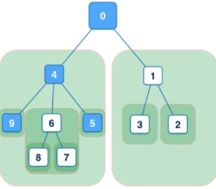
labeled asyk from leaf node setL instead ofY. One implication for this is illustrated

(40)

the root node if it is categorized to node 4. Let a path denotes a set of labels with parent-child relations, and for every instancexk, letPath(k) be thepath that includes

yk. Then in this case Path(k) will be {4,1,0} (remember 0 is the root node). If we

further assume that all the instances are categorized until it is found in one and only one leaf node, this leaf node alone is enough to represent the whole path an instance is attached with, which is why we assign every instance only one label yk. So in

previous example,yk is 4, the index of leaf node isxk classified to.

The challenge here is to learn a function f :X → Y that is efficient to train and easy to test. Assuming for each node i ∈ Y a vector wi ∈ Rp has been given, a

top-down procedure is utilized to classify an instance from the root to one leaf node [34, 36, 41, 42].

Algorithm 1: Top-Down Procedure for Classification

1 Inputs: {C(i)}m_i₌₁,{w_i}m_i₌₁, x_k 2 Outputs: i

3 LET i←0

4 while C(i) is not empty do

5 LET i = arg max

j∈C(i)

wT_jxk

What Algorithm 1 is trying to do is to assign one leaf node to every unknown instance. Given any node i an instance xk belongs to, Algorithm 1 classifies xk

among S+₍_i_{), updating} _i _{and repeating the procedure until} _i _{is a leaf node. In this}

way we decouple the problem into a series of multi-class classification problems at each level.

There are different methods to train multi-class classifiers, either one-versus-rest, one-versus-one or solving a single optimization problem [38]. In this paper, we have adopted the one-against-rest approach, where for each node i, a binary classification problem is solved independently to learn a classifier that is responsible for predicting the membership of an instance against S+₍_i_{). Let} _T₍_i_{) =}_{_k _| ₍_x

k, yk) whereP(i)⊂

(41)

Figure 2.1: The hierarchy tree of the labels.

we define for each node i∈Y¯ and k∈ T(i)

y_k(i) =    1 i∈ Path(k) −1 otherwise then the training set for node i would be

¯

X(i) = {(xk, y

(i)

k ) | k∈ T(i)} (2.3.2)

The procedures are schematized in Algorithm 2.

Algorithm 2: Independent Classifiers Training

1 Inputs: ¯Y,{(xk, yk)}Nk=1

2 Outputs: {w_i}m_i₌₁ 3 for i= 0→m do

4 Construct training set ¯X(i)

5 Training

6 Save w_i

2.3.2

A Novel Hybrid Approach

As motivated in Section 5.1, we want to build a hierarchical classification system that (1) provides scalability and portability, (2) imposes consistency in parent-child rela-tions, (3) reduces inaccuracy in training classifier for each node, (4) adapts tailored

(42)

models and algorithms to each node based on different conditions and requirements. While the first two points are addressed in Section 2.3 by introducing the top-down classifying procedure and independent training approach for each node, the last prob-lem that is essential to the system’s overall speed and accuracy is taken care of by our novel hybrid approach presented in this section. As mentioned in Section 2.3, in most hierarchical classification problems there are a large amount of data at the high levels of the class hierarchy, and the sizes the training sets are considerably smaller at the low levels as the classes become much more specific. The difference in problem sizes at nodes of different levels presents us with different challenges and emphases in solving the underlying optimization problem. In particular, for those nodes with large amount of data, a small generalization error of the model is inherently easy to obtain since more information is presented to the model. But the resulting optimiza-tion problem becomes very large and thus brings about computaoptimiza-tional difficulties. On the other hand, for those nodes with scarcity of data, it is relatively easy to solve the optimization problem but a more accurate solution is required to compensate for the lack of training information.

Regarding that, we present our novel hybrid approach, which combines the co-ordinate descent methods and the IPM algorithm in the hierarchical classification framework. Ideally we can use one algorithm from top to bottom if there exists such an algorithm that outperform others both in speed and accuracy. In fact this is what people have been using in practice most of the time, and Interior Point Methods (IPM) with its fast convergence rate makes such a good candidate, demonstrating satisfying performance as long as the size of the problem is small. However, the need to solve a Newton system markedly limits the scalability of IPM-based algorithm since the time and memory it takes to solve the Newton system at every iteration increases substantially as the problem size becomes large. Hence, we only use an IPM-based method as the problem becomes small enough, i.e. when we reach the bottom level of the hierarchy. For the top level of the hierarchy where the problem size is often much larger than that of bottom-level problems, in order to train the classifiers efficiently,

(43)

we consider the two variants of coordinate descent methods.

Software Architecture The HiClass system is the combination and

implementa-tion of what we have discussed in previous secimplementa-tions, including the hierarchical classifi-cation framework and our novel hybrid approach with the implementation of IPM by [10], the first order coordinate descent by [9] called SCD and the second order variant by [32] called GLMNET, to solve the hierarchical classification problems accurately and efficiently. The strength of our HiClass system is that it is designed to be highly modular and flexible. The core of the system consists of four basic modules:

1. Hierarchy TreeThe tree module implements the framework described in

Sec-tion 2.3 and forms the foundaSec-tion of the system.

2. Data ReaderThe reader module reads the data from text files of different

for-mats (e.g. LIBSVM or UCI) and stores it in matrix and vector data structures in the memory.

3. QP Writer The writer module transforms the raw data into the appropriate

matrices and vectors and writes them in the format required by different solvers as the input file.

4. Solver Engine The solver engine provides implementation for the algorithms

described above.

Figure 2.2 shows the general architecture of the software system. Given the training data sets and the hierarchical structure of the labels, HiClass problem read transfers those data in memory to HiTree data, which then distribute to every node a different training set (as defined in (2.3.2)) that are necessary for the solvers to compute the classifier of that node. HiClass node write interfaces with the data and the solvers that consists of GLMNET used in the top (first) level of the hierarchy along with IPM for the rest. Note that the process is easy to parallelize since every classifier for each node is trained independently, as illustrated in the figure.

(44)

Figure 2.2: HiClass system flow chart

2.3.3

Experiments

In this section, we first discuss the measure of performance we use in every node of hierarchy and we test the performance of HiClass on real-world data set.

The Evaluation Metrics

To evaluate the performance of the HiClass system, we use the micro-average F1

measure [43]. On a single category the Fβ is given by

Fβ =

(β2 _{+ 1)}_A

(β2_{+ 1)}_A₊_B₊_β2_C, (2.3.3)

where A is the number of documents a system correctly assigns to the category (true positives), B is the number of documents a system incorrectly assigns to the category (false positives), and C is the number of documents that belong to the category but which the system does not assign to the category (false negatives). Let β= 1.0, then

(45)

we have the harmonic mean of recall and precision: F1 = 2A 2A+B +C = 2RP R+P, (2.3.4)

where R is recall, i.e., A/(A+C), and P is precision, i.e., A/(A+B).

In our case, every category i will have its own Ai, Bi and Ci. There are two

methods, called macro-average and micro-average to combine those statistics into one measure in order to evaluate the general performance on the hierarchical structure. If we have category from 1 to l, then macro-average F1 is just the unweighted mean

of F-measure across all categories

macroF1 =

Pl

i=1(F1)i

l (2.3.5)

and micro-average F1 is given by

microF1 = 2Pl i=1Ai Pl i=12Ai+Bi+Ci (2.3.6) In fact, (2.3.6) can be simplified. Since Pl

i=1Ai+Ci =N where N is the number of

all test instances. But we also have Pl

i=1Ai+Bi =N. Therefore, l X i=1 2Ai+Bi+Ci = 2 l X i=1 (Ai +Ci) = 2N

so (2.3.6) is in fact the ratio of true positives and total number of instancesmicroF1 =

Pl

i=1Ai

N .

The RCV1 Dataset

The RCV1-v2/LYRL2004 is a text categorization test collection made available from Reuters Corpus Volume I (RCV1), an archive of over 800,000 manually categorized newswire stories [43]. Each RCV1-v2 document used in our experiment has been tokenized, stopworded, stemmed and represented by 47,236 features in a final form as ltc weighted vectors. Those RCV1 documents are categorized with respect to the

(46)

Topics, which were organized in four hierarchical groups: CCAT, ECAT, GCAT and MCAT.

The RCV1-v2 documents are split chronologically into a training set and test set, with 23,149 training documents and 781,265 test documents. For our experiments, we focus on CCAT and MCAT two subtrees. The ECAT and GCAT subtrees are not considered because the former has a similar tree structure with CCAT and the latter display a structure that is flat rather than organized hierarchically. During preprocessing, we discard those that are not associated with any those leaf nodes as well as those that are categorized to multiple ones, requiring that each document used in the experiments is categorized to exactly one leaf node of either CCAT or MCAT. Next we discuss details.

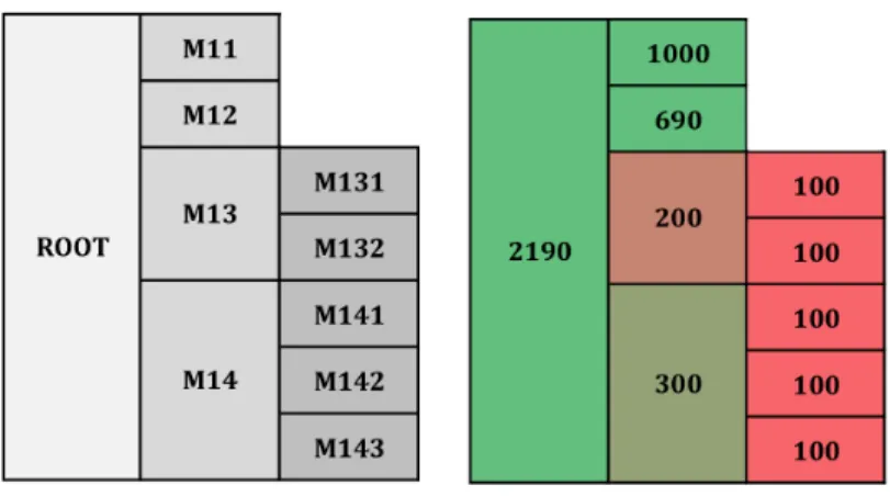
(a) CCAT hierarchical struc-ture. Each node in the tree is represented here as a block in the table. For example, C17 is the child of ROOT and has four children named from C171 to C174.

(b) The training data we use for classification at each node. The unbalanced data distribu-tion problem we mendistribu-tioned be-fore is obvious here, with abun-dant amount of data for upper nodes yet much less at ones in the bottom.

Figure 2.3: CCAT subtree

Experiments on the CCAT Subtree We trim the CCAT topic group for our

(47)

one child. Reserving the main structure of CCAT, we end up with topics organized in a tree illustrated in Figure 2.3(a). There are altogether 17 nodes including 13 leaf nodes, 3 internal nodes and 1 root. The number of training data for each topic

is illustrated in Figure 2.3(b) where the color shifts from green to red with more green denoting larger numbers. The total number is 2062 and most of them amass in the first hierarchy, which causes the previously mentioned unbalanced data dis-tribution problem. In the experiments, we run including our HYBRID method all four algorithms with the same stopping criteria and same regularization parameter. The accuracy (using micro-average F1 measure [43]) and cpu time are recorded for

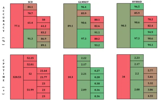
each node respectively and for the whole tree as well. The results are presented in Figure 2.4.

The first thing to note from Figure 2.4 is that the more second order information we take into consideration, the more accuracy we eventually achieve as expected, which can be seen by comparing the accuracy obtained by GLMNET, a second-order algorithm, with that of SCD which completely ignores the Hessian information. It can be seen that the first-order method SCD actually takes much longer than GLMNET to solve the problem, e.g., 556s compared with 17s. Having examined the detailed printouts of each algorithm, we find that even though SCD enjoys cheap per iteration cost, it takes SCD a lot more iterations than GLMNET to be able to satisfy the same stopping criteria, mostly due to the small step size SCD is forced to take each iteration. And the step size of SCD is inevitably small mainly because the lack of second order information forces it to build a globally upper bound model locally, which is thus a very loose bound with the minimizer too close to the current iterate. Hence, SCD progresses slowly, eventually resulting in expensive total computational cost even though each step only takes constant time.

On the other hand, GLMNET solves the problem very fast, e.g., nearly 35 times faster than SCD. The importance of curvature information can be further appreciated comparing the performance of GLMNET with that of SCD. Particularly, by incor-porating second order information into the algorithm, GLMNET is able to achieve

(48)

Figure 2.4: Performance comparison at each node between above mentioned algorithms. For HYBRID, we use GLMNET in the upper level and IPM at bottom. The number in the leftmost block of each table denotes the corresponding perfor-mance measure on the whole tree. For example, as shown by the rightmost upper table, 70% aggregate accuracy is achieved using the novel HYBRID method.

the fast convergence rate comparable to that of IPM; plus the cheap iteration cost similar to that of SCD, it is expected that GLMNET performs efficiently. However, GLMNET is not as accurate as IPM and although the inaccuracy can be somehow compensated by the abundance of training at the first hierarchy, the problem becomes more serious as it goes down the tree, e.g., almost 30% loss of accuracy in some cases. Finally, by combining different algorithms we obtain a HYBRID method that has better accuracy than GLMNET. It is expected that the time HYBRID takes is over 90% less than that spent by SCD, due to not only the use of GLMNET in the first hierarchy, but also the fact that IPM at the bottom performs efficiently with

(49)

limited amount of data as well. In fact, the saving can be much more when the data distribution is more severely unbalanced, in which case there are much more data in the first level and the number decreases dramatically at the bottom. As a result, the time IPM takes to solve the problem increases much faster than that of GLMNET, mainly due to IPM’s per iteration complexity growing quadratically with the number of training points. The advantage of using HYBRID will become more obvious in those cases. Another thing to note is the accuracy HYBRID achieves, which is the highest of all. Again, as we discussed, the use of IPM at the bottom improves the accuracy of GLMNET and the use of GLMNET at the upper level returns a slightly better accuracy than IPM because the ability of GLMNET to efficiently process large scale of data.

(a) MCAT hierarchical struc-ture.

(b) The training data we use for classification at each node.

Figure 2.5: MCAT subtree

Experiments on the MCAT Subtree The whole experiment setting is similar to

that of CCAT, except that this time we have a different hierarchical structure. The MCAT subtree contains altogether 9 nodes including 7 leaf nodes, 2 internal nodes and 1 root node, as illustrated in Figure 2.5(a). The number of training documents labelled under eachtopics is shown in Figure 2.5(b), from which we can see that over

(50)

75% of the data are accumulating on M11 and M12. We therefore expect that IPM will have a hard time at the first level where the data matrix has more than 2000 rows and 47326 columns. In fact, it does take IPM too long to solve the problem such that we can’t include the results in Figure 2.6. But we are still able to use IPM in the HYBRID method because the problem size at the bottom is at most 300, which is comfortably within the range of IPM.

Figure 2.6: Performance comparison at each node between