Efficien and Scalable Data Evolution with Column Oriented Databases

Efficien and Scalable Data Evolution with

Column Oriented Databases

Ziyang Liu

, Bin He

, Hui-I Hsiao

, Yi Chen

ziyang.liu@asu.edu, binhe@us.ibm.com, hhsiao@almaden.ibm.com, yi@asu.edu

ABSTRACT

Database evolution is the process of updating the schema of a database or data warehouse (schema evolution) and e-volving the data to the updated schema (data evolution). It is often desired or necessitated when changes occur to the data or the query workload, the initial schema was not carefully designed, or more knowledge of the database is known and a better schema is concluded. The Wikipedia database, for example, has had more than 170 versions in the past 5 years [8]. Unfortunately, although much research has been done on the schema evolution part, data evolu-tion has long been a prohibitively expensive process, which essentially evolves the data by executing SQL queries and re-constructing indexes. This prevents databases from being flexibly and frequently changed based on the need and forces schema designers, who cannot afford mistakes, to be high-ly cautious. Techniques that enable efficient data evolution will undoubtedly make life much easier.

In this paper, we study the efficiency of data evolution, and discuss the techniques for data evolution on column ori-ented databases, which store each attribute, rather than each tuple, contiguously. We show that column oriented databases have a better potential than traditional row ori-ented databases for supporting data evolution, and propose a novel data-level data evolution framework on column ori-ented databases. Our approach, as suggested by experimen-tal evaluations on real and synthetic data, is much more efficient than the query-level data evolution on both row and column oriented databases, which involves unnecessary access of irrelevant data, materializing intermediate results and re-constructing indexes.

Categories and Subject Descriptors

H.2.4 [Systems]: Relational databases

General Terms

Algorithms, Performance

Permission to make digital or hard copies of all or part of this work for personal or classroom use is granted without fee provided that copies are not made or distributed for profi or commercial advantage and that copies bear this notice and the full citation on the firs page. To copy otherwise, to republish, to post on servers or to redistribute to lists, requires prior specifi permission and/or a fee.

EDBT 2011, March 22–24, 2011, Uppsala, Sweden. Copyright 2011 ACM 978-1-4503-0528-0/11/0003 ...$10.00

Keywords

column oriented database, bitmap index, schema, data evo-lution

1. INTRODUCTION

Database evolution is the process of updating the schema of a database/data warehouse (schema evolution) and evolv-ing the data to the new schema (data evolution). The needs of database evolution arise frequently in modern databas-es [16, 15, 27, 29] and data warehousdatabas-es [10, 18] in both OLTP and OLAP applications due to emerging of new knowledge about data and/or changes in workload, and from both new application demand perspective and analytical experiments perspective. As observed by Curino et. al [16], “the serious problems encountered by traditional information system-s are now further exacerbated in web information system-sysystem-stemsystem-s and cooperative scientific databases where the frequency of schema changes has increased while tolerance for downtimes has nearly disappeared.”

For instance, the Ensembl Genetic DB has involved in over 400 schema changes in nine years [16]. Another ex-ample is a data warehouse containing raw data and derived data (analytical results on the raw data). Since there are more and more new analytical requirements nowadays, the derived data and their schema often become complex and frequently evolving. Even for a single analytical task, it is also often true that it may take some time to develop and ex-periment before being stabilized, which will generate many schemas during the process. Consider a patent database as an example. In the first round of building an annotator to extract chemical compounds from patents, we may extrac-t SMILES1 in the patents, chemical names and the corre-sponding usages. Later on, we may want to put SMILE and chemical name attributes into a separate table to reduce the redundant information [13].

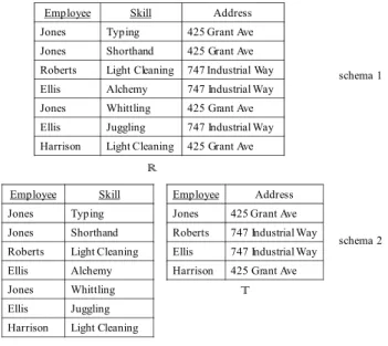
In general, a database evolution may be desired or neces-sitated when new information about the data and/or the workload emerges. In the remainder of this paper we use the tables in Figure 1 as a simplified example to illustrate the motivation and the proposed methodologies.

1. New Information about the Data. In a dynamic application scenario, new information about the da-ta may become available, which requires to update, add or remove attributes in a database, as well as re-organize the table structure. Consider tableRin

Employee Skill Address Jones Typing 425 Grant Ave Jones Shorthand 425 Grant Ave Roberts Light Cleaning 747 Industrial Way Ellis Alchemy 747 Industrial Way Jones Whittling 425 Grant Ave Ellis Juggling 747 Industrial Way Harrison Light Cleaning 425 Grant Ave

Employee Address Jones 425 Grant Ave Roberts 747 Industrial Way Ellis 747 Industrial Way Harrison 425 Grant Ave Employee Skill

Jones Typing Jones Shorthand Roberts Light Cleaning Ellis Alchemy Jones Whittling Ellis Juggling Harrison Light Cleaning

S

T R

schema 1

schema 2

Figure 1: Example of Database Evolution

ure 1. Suppose originally, it only has attributes Em-ployee and Skill. If later on the address information emerges, we would like to add anattributeAddressto

R. Furthermore, at the schema design time, the de-signer might have believed that each Employeehas a single Skill. When more data tuples are added, it is revealed that each employee may have multiple skill-s. Thus it is better to decompose R to two tables

S and T, as shown in schema 2, in order to preven-t dapreven-ta redundancy and updapreven-te anomaly. As we can see, updating the data content may reveal or invali-date functional dependencies that may not be known when the schema was originally designed, and thus re-quires schema changes.

2. New Information about the Workload. Query

and update workload of a database may vary from time to time. Different workloads may have different da-ta access patterns, and demand different schemas for optimized performance. Consider Figure 1 again, as-sume that the original workload is update intensive, for which Schema 2 is desirable. Later workload charac-teristics change and become query intensive, and most queries look for addresses given skills. Now Schema 1 becomes more suitable, as it avoids joins of two tables. A database evolution involves both updating the schema of a database and evolving the data to the new schema. Existing work on database evolution mainly studies schema evolution and its effects [15, 27, 11, 14, 20, 34, 37]. However, efficient algorithms to actually evolve the data to the new schema has yet to be developed. Currently data evolution is performed atquery-level, expressed and implemented by SQL queries [26]. As an example, the following SQL queries can be executed to evolve the data from R to S and T in Figure 1:

1. insert intoS select Employee, Skill fromR

2. insert intoTselect distinct Employee, Address

from R

Such a query-level data evolution framework is notorious-ly inefficient in terms of both time and space for two rea-sons. First, it has excessive data accesses; every (distinct) attribute value in every tuple is accessed. Second, after the query results are loaded into the new tables, indexes have to be built from scratch on the new table. This approach makes data evolution prohibitively expensive and even inapplica-ble, as to be shown in this paper and is also observed in [15]. The inflexibility of schema change on current database sys-tems not only results in degraded system performance over time, but forces schema designers to be highly cautious and thus severely limits the database usability [21].

In this paper, we study the problem of efficient data evolu-tion in designing an agile database system. Ideally, an agile data evolution should minimize data accesses; and it is also desirable if we can derive the new indexes from the original indexes, rather than constructing the indexes on the new table from scratch.

To minimize data accesses, we observe that when chang-ing the database schema, usually many columns in a table remain unchanged. For example, the columns in tableSin Figure 1 are exactly the same as the corresponding ones in

R, thus these columns are unchanged during the decompo-sition from R to S and T. As a result, a column-oriented database, or column store, becomes a natural choice for ef-ficient data evolution. In a column-oriented database, each column, rather than each row, is stored continuously on the storage. Column stores usually outperforms row stores for OLAP workloads, and studies have shown that column s-tores fit OLTP applications as well [6, 33].

However, performing a query-level data evolution on a column oriented database is still very expensive. First, we need to generate query results, during which the columns need to be assembled into tuples; second, result tuples need to be disassembled into columns; at last, each column of the results needs to be re-compressed and stored. These steps incur high costs, as to be shown in Section 5.

To address these issues, we propose a framework of data-level data evolution on column oriented databases, which achieves storage to storage data evolution without involv-ing queries. A system of our data level approach has been demonstrated in VLDB ’10 [25]. We support various opera-tions of schema changes, among which two important ones, decomposing a table and merging tables, are the focus of this paper. We design algorithms that exploit the char-acteristics of column oriented storage to optimize the data evolution process for better efficiency and scalability. Our approach only accesses the portion of the data that is af-fected by the data evolution, and has the unique advantages of avoiding SQL query execution and data decompression and compression. We report a comprehensive study of the proposed data evolution algorithms on column oriented s-torages, compared with the traditional query-level data evo-lution. Experiments show that data-level data evolution on column oriented databases can be orders of magnitude faster than query-level data evolution on both row and column ori-ented storages for the same data and schemas. Besides, it is observed that our approach is more scalable, while the per-formance of query-level data evolution deteriorates quickly when the data become large. Our results bring a new per-spective to help users make choices between column orient-ed storage and row orientorient-ed storage, considering both query processing and database evolution needs. Due to the

advan-tage in data evolution, column stores may get an edge over row stores even for OLTP workloads in certain applications.

Our contributions in this paper are summarized as: 1. This is, to the best of our knowledge, the first study

of data evolution on column oriented storages, and the first on designing algorithms for efficient data-level evolution, in contrast to the traditional query-level da-ta evolution. Our techniques make dada-tabase evolution a more feasible option. Furthermore, our results bring a new perspective to help users make choices between column oriented storage and row oriented storage, con-sidering both query processing and database evolution needs.

2. We propose a novel data-level data evolution frame-work that exploits column oriented storages. This ap-proach only accesses the portion of the data that is affected by the data evolution, and has the unique ad-vantages of avoiding SQL query execution, indexes re-construction from the query result, and data decom-pression and comdecom-pression.

3. We have performed comprehensive experiments to e-valuate our approach, and compared it with traditional query-level data evolution, which show that our ap-proach achieves remarkable improvement in efficiency and scalability.

The following sections of this paper are structured as: Sec-tion 2 introduces necessary backgrounds on column orient-ed databases and the types of schema changes. Then we present the algorithms for two important types of schema change: decomposition (Section 3) and merging (Section 4). We report the results of experimental evaluations to test the efficiency of data evolution in Section 5. Section 6 discusses related works and Section 7 concludes the paper.

2. PRELIMINARIES

2.1 Column Oriented Databases

Unlike traditional DBMSs which store tuples contiguous-ly, column oriented databases store each column together. Column store improves the efficiency of answering queries, as most queries only access a subset of the columns, and therefore storing each column contiguously avoids loading unnecessary data into memory. In addition, as values in a column are often duplicate and/or similar, compression and/or encoding technologies can be applied in column s-tores to reduce the storage size and I/O time.

Studies show that column store is suitable for read-mostly queries typically seen in OLAP workloads, and it is a good choice for many other application scenarios, e.g., databases with wide tables and sparse tables [3], vertically partitioned RDF data [4], etc. In these applications, schema evolution is common. For instance, in OLAP applications, a warehouse may add/delete dimensions. When new data or workload emerges, a warehouse may want to evolve a dimension from star schema to snowflake schema (or verse visa), which is exactly the decomposition (or merging) operations studied in this paper. This paper proposes novel techniques that efficiently support schema evolution in column stores.

Bitmap is the most common encoding scheme used in col-umn stores [5]. The state-of-the-art bitmap compression

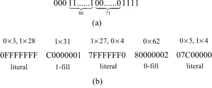
86 71 000 11...100...01111 (a) 0 3, 1 28× × 0FFFFFFF literal 1 31× C0000001 1-fill 7FFFFFF0 literal 1 27, 0 4× × 07C00000 literal 0 5, 1 4× × (b) 80000002 0-fill 0 62×

Figure 2: WAH Compression of Bitmap

methods and encoding strategies have made bitmap index-es widely applicable. Modern bitmap indexindex-es can be ap-plied on all types of attributes (e.g., high-cardinality cate-gorical attributes [35], numeric attributes [28] and text at-tributes [32]). Studies show that a compressed bitmap index occupies less space than the raw data and provides better query performance for equal queries [36], range queries [35], and keyword queries [32]. Besides, [36] shows that with proper compression, bitmaps perform well for columns with cardinality up to 55% of the number of rows, indicating that they can be widely adopted. Nowadays, bitmap indexing is supported in many commercial database systems (e.g, Or-acle, Sybase, Informix), and is often the default (or only) indexing option in column-oriented database systems (e.g., Vertica, CStore, LucidDB), especially for applications with read-mostly or append-only data, such as OLAP applica-tions and data warehouses. In this paper we assume that, unless an attribute (also referred to as a column) is a pri-mary key, it is compressed using bitmap encoding.2

Various compression methods for bitmaps have been pro-posed. Among those, Word-Aligned Hybrid (WAH) [36], Position List Word Aligned Hybrid [17] and Byte-aligned Bitmap Code (BBC) [9] can be applied to any column and be used in query processing without decompression. We adop-t Word-Aligned Hybrid (WAH) adop-to compress adop-the biadop-tmaps in our implementation. In contrast, run length compres-sion [33] can be used only for sorted columns.

WAH organizes the bits in a vector by words. A word can be either a literal word or a fill word, distinguished by the highest bit: 0 for literal word, 1 for fill word. Let L denote the word length in a machine. A literal word encodes

L−1 bits, literally. A fill word is either a 0-fill or a 1-fill, depending on the second highest bit, 0 for 0-fill and 1 for 1-fill. LetN be the integer denoted by the remainingL−2 bits, then a fill word represents (L−1)×N consecutive 0s or 1s. For example, the bitmap vector shown in Figure 2(a) is WAH-compressed into the one in Figure 2(b).

In order to find the corresponding vector in a bitmap given a value in a column, we use a hash table for each column to map from each value to the position of the vector. The number of entries in the hash table is the number of distinct values in the column. We also build an offset index similar to the one in [33] for each bitmap to find the value in a column given a position.

2_{Other compression schemes are sometimes used for special}

columns, such as run length encoding for sorted column-s. In this paper we focus on the general case with bitmap encodings for all non-key attributes. Supporting other com-pression/encoding schemes is one of our future works.

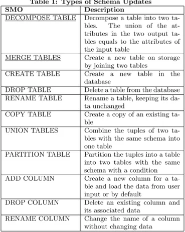
Table 1: Types of Schema Updates

SMO Description

DECOMPOSE TABLE Decompose a table into two ta-bles. The union of the at-tributes in the two output ta-bles equals to the attributes of the input table

MERGE TABLES Create a new table on storage by joining two tables

CREATE TABLE Create a new table in the database

DROP TABLE Delete a table from the database RENAME TABLE Rename a table, keeping its

da-ta unchanged

COPY TABLE Create a copy of an existing ta-ble

UNION TABLES Combine the tuples of two ta-bles with the same schema into one table

PARTITION TABLE Partition the tuples into a table into two tables with the same schema with a condition ADD COLUMN Create a new column for a

ta-ble and load the data from user input or by default

DROP COLUMN Delete an existing column and its associated data

RENAME COLUMN Change the name of a column without changing data

2.2 Schema Updates

We support all the Schema Modification Operators (S-MO) introduced in [15], which are listed in Table 1. Create, Drop, and Rename Table operations incur mainly schema level operations and are straightforward. Copy, Union and Partition Table operations require data movement, but no data change. Thus existing approaches for data movemen-t can be applied. For column level SMO, especially Add Column and Drop Column, column oriented databases have obvious advantages, as data in other columns do not need to be accessed. In this paper, we discuss Decompose and Merge in details. We will propose algorithms for efficient de-composition and merging, and show empirically that these operations are much more efficient on column stores than on row stores.

Decomposition.This operation decomposes a table into two tables. As an example, see Figure 1. TableRis decom-posed into two tables (SandT). We assume that a decompo-sition is lossless [31], since only a lossless-join decompodecompo-sition ensures that the original table can be reconstructed based on the decomposed tables. In a lossless-join decomposition of table Rinto S and T, the common attributes of S and

Tmust include a candidate key of either S or T, or both. Decomposing a table into multiple tables can be done by recursively executing this operation.

Merging. It joins two tables to form a new table, such asSandTin Figure 1 intoR. Merging multiple tables can be done by recursively executing this operation.

Next, we will discuss the data-level evolution algorithms for decomposition and merging respectively in Section 3 and Section 4.

3. DECOMPOSING A TABLE

In this section we discuss the details of lossless-join de-composition. We useRto denote the original table, andS,

Tto denote the two output tables.

We start by introducing two critical properties of a lossless-join decomposition which will be exploited by our algorithm-s:

Property 1: In a lossless-join decomposition which decom-poses a table into two, at least one of the two output tables has the same number of rows as the input table.

Property 2: For an output table with a different number of rows as the input table, its non-key attributes have func-tional dependency on its key attributes in the original table. Now we prove these two properties. Without loss of gen-erality, let Rdenote the input table and S, T the output tables. By the definition of lossless-join decomposition, the common attributes ofSandTmust include a candidate key of either Sor T. Suppose the common attributes, denoted byAc, are a candidate key ofT. Then if we join S andT, since they join onAcand each tuple ofThas a unique value ofA_c, each tuple inScan have at most one matching tuple inT. Therefore,Shas the same number of rows as the input tableR, and property 1 holds. Furthermore, since the join is essentially extending each ofT’s key value withS’s matching non-key attributes, thus for any ofT’s key values inR, the corresponding T’s non-key values should be the same, and thus Property 2 holds.

Property 1 can be effectively utilized by column oriented databases. Since each column is stored separately, the un-changed output table can be created right away using the existing columns inRwithout any data operation. Column-store makes it possible to only access the data that is neces-sary to change in data evolution, and thus save computation time.

3.1 Algorithm Overview

In our algorithm description below, let the set of attributes in R,S,T be (A1, · · ·, Ak, Ak+1, · · ·, An), (A1, · · ·, Ak,

Ak+1,· · ·,Ap), and (A1,· · ·,Ak,Ap+1,· · ·,An) respective-ly. Assume that the common attributes ofSandT,A1,· · ·,

Ak, comprise the key ofT, which meansSis the unchanged

output table.

Intuitively, to generateT, we can take the following steps: 1) For each distinct value v of T’s key attributes A1, · · ·,

Ak, we locate a tuple position in Rthat contains v. The result of this step is a list of tuple positions in R, one for each distinct value ofT’s key attributes.

Eachvpresents a list ofkvalues fromT’s key attributes. Because of Property 2, all tuples inRwith the samevhave the same values onAp+1,· · ·,An. We thus can choose any one of these tuples and do not need to access all of them. 2) Given the position list, we can directly generate new bitmaps ofT’s attributes from their corresponding bitmaps inR. That is, for each attribute, we can shrink their bitmap inRby only taking the bits specified in the position list. We name such an operation as “bitmap filtering”.

During this process, the hash and offset index for each of

T’s attributes are also updated. After we shrink each vec-tor using the bitmap filtering operation, we insert an entry to the corresponding hash table for the attribute, recording

the position of the shrunk vector. For each position in the position list, we access the offset index of the original at-tribute (inR) to retrieve the attribute value, and insert an entry accordingly to the corresponding offset index for the attribute inT.

The pseudo-code for the above two steps is presented in Algorithm 1. Step one is realized by calling adistinction

function, which is to be described in Section 3.2. It returns

keyvalues, which records the distinct values ofA1,· · ·, Ak, andkeypos, storing one position of each of these values inR. The positions inkeyposare then sorted to support efficient search in step two.

Example 3.1. In Figure 1, the key of table T is a sin-gle attributeEmployee. We first compute its distinct values stored in keyvalues, which are Jones, Roberts, Ellis and

Harrison. We also find one position of each of them in R stored inkeypos, which are, for example, rows 1, 3, 4 and 7 respectively.

In step two (lines 3-9 of Algorithm 1), WhenT only has one key attributeA1 (i.e., k = 1), it is unnecessary to s-tore A1 with a bitmap structure as each A1’s value only occurs once. We thus simply output the distinct values in

keyvalues(line 4). For other cases and non-key attributes, we conduct the “bitmap filtering” operation for each at-tribute. The details of thefilteringoperation is described in Section 3.3. It is easy to see that, since we deal with one attribute at a time in step two, the number of attributes to be processed does not bring a memory constraint for our algorithm.

Algorithm 1Decomposing a Table

Decompose₍R_(A1,· · ·_{, An), k, p)}

Output: T(A₁,· · ·, A_k, A_p+1,· · ·, A_n)

1: keyvalues, keypos=distinction(R, A1,· · ·, A_k)

2: sortkeypos 3: ifk= 1then 4: A₁=output(keyvalues) 5: else 6: fori= 1 tokdo 7: A_i=filtering(Ai, keypos) 8: fori=p+ 1 tondo 9: A_i=filtering(A_i, keypos)

Example _{3.2. In the running example, table}T _{has a} s-ingle key attribute: Employee. According to line 4 of Algo-rithm 1, columnEmployeein table Tconsists of the values inkeyvalues, which areJones, Roberts, EllisandHarrison. Given the list of positions keypos = {1,3,4,7}, in or-der to generate column Address in the output table T, we need to perform a filtering operation on columnAddressin R. There are two vectors for this attribute, corresponding to

425 Grant Aveand747 Industrial Way. Their vectors in the bitmap are 1100101 and 0011010 respectively. We retrieve the values of the two vectors at positions 1, 3, 4 and 7. For

425 Grant Ave, the values are 1001, and for 747 Industri-al Way the values are 0110. Therefore, the new bitmap of

Addressconsists of two vectors, 1001 and 0110.

Next we discuss the two procedures involved in a decom-position,distinctionandfiltering, in details.

3.2 Distinction

We start with the easier case – distinction on a single attribute, such as attributeEmployeein Figure 1. Since the attribute on whichdistinctionis performed is not the key of tableR, it is encoded as a bitmap structure.

Algorithm 2Distinction on a Single AttributeA

Distinction_{(Bitmap of AttributeA)} Output: keyvalues, keypos

1: keyvalues=∅

2: keypos=∅

3: foreach distinct valuevofAdo

4: vec=v’s vector inA’s bitmap

5: elapsed= 0

6: fori= 1 tovec.sizedo

7: if vec[i] is a literal wordthen

8: j= position of the first seen 1-value bit invec[i]

9: keypos=keypos∪ {elapsed+j}

10: keyvalues=keyvalues∪ {v}

11: break

12: else ifvec[i] is a 1-fill wordthen

13: keypos=keypos∪ {elapsed+ 1}

14: keyvalues=keyvalues∪ {v}

15: break

16: else

17: N= the number of 0s encoded invec[i]

18: elapsed+=N

19: returnkeyvalues,keypos

Algorithm 2 presents the steps for distinction on a single column, denoted asA. Recall thatA’s bitmap has a vector for each of A’s distinct values, and therefore the bitmap directly gives the distinct values ofA. To find the position of each distinct value, we traverseA’s value→vector position hash; for each ofA’s distinct valuev, we locate the position ofv’s vector (line 4), and then find the position of the first “1” in the vector (lines 6-18), which is the position of the first occurrence of v in column A (recall that actually the position of any other “1” can be used). The position of the first “1” in each vector is stored in array keypos and the distinct values inkeyvalues.

To find the position of the first “1” for each distinct value, we can simply scan each vector. We notice that in a bitmap compressed using WAH, the first “1” of any vector always appears in the first two words, unless the table has more than 31×230 (≈ 30 billion) rows (assuming the machine word length is 32), which is rarely seen. Therefore in the majority of cases, we do not need to access the entire bitmap of a column at all. Instead, we can additionally record the first two words of each vector in the bitmap in a separate file, called the snapshotof the bitmap. When we perform distinction on this column, this file can be used instead of the bitmap itself to find the position of the first “1” in each vector. The snapshot file is tiny compared to the bitmap, as regardless of the length of the bitmap vector, in a snapshot each vector has only two words.

When there are more than one key attribute, we cannot directly get distinct values from the bitmap, as the bitmap is constructed on a per attribute basis. There are two ways to deal with this case. The first method is to combine bitmaps of multiple attributes. Consider two attributes A and B, each encoded as a bitmap. For each value vA of A and

vB ofB, if we perform an AND operation on their vectors,

the resulting vector indicates the position wherevA andvB

vector ofA and B and keep the non-zero vectors, we can get the distinct values of (A, B) and their positions with similar process of Algorithm 2. It is easy to generalize this method on three or more attributes. This approach works well ifAandBhave a small number of distinct values, as its processing time is proportional to the product of the number ofA’s distinct values and the number ofB’s distinct values. As an alternative, we can also scan the offset index of the involved columns to access each row of these columns, and use hashing to recognize each distinct values during the scan.

3.3 Filtering

The filtering operation generates a new bitmap of an at-tribute given its original bitmap and a list of positions,

keypos. Each vector in the new bitmap only contains rows specified bykeyposin the original bitmap, and thus this op-eration can be considered as “filtering” the original bitmap.

Algorithm 3Filtering a Bitmap Based on a List of Posi-tions

Filtering(Bitmap and offset index for AttributeA,keypos) Output: the filtered bitmaptgtBitmap, the new hashtgtHash and offset indextgtOffset

1: foreach vectorvecofA’s bitmapdo

2: vec= an empty vector

3: elapsed= 0

4: currpos= 1

5: fori= 1 tovec.sizedo

6: ifvec[i] is a literal wordthen

7: elapsed+= 31

8: whilecurrpos≤keypos.sizeandkeypos[currpos]≤ elapseddo

9: add the (keypos[currpos]−elapsed)th bit ofvec[i] tovec

10: encode the new added bits in the vector vec if necessary using WAH encoding

11: currpos++

12: else

13: elapsed+= the number of 0s (1s) encoded invec[i]

14: endpos= use a binary search to find the largest po-sition inkeypossatisfyingkeypos[endpos]≤elapsed

15: add (endpos−currpos+ 1) 0s (1s) to the vectorvec

16: encode the new added bits in the vector vec if nec-essary using WAH encoding

17: currpos=endpos+ 1

18: add the vectorvec totgtBitmap

19: add the position oftgtBitmaptotgtHash

20: fori= 1 tokeypos.sizedo

21: value= the value ofAat rowkeypos[i]

22: add entry (i, value) intotgtOffset

23: returntgtBitmap

The algorithm for the filtering operation is shown in Al-gorithm 3. For each vectorvecof attribute A, we traverse the list of positionskeypos. Specifically, for each wordvec[i] invec, if it is a 0-fill or a 1-fill word, we directly jump from the current position inkeyposto the largest position that is still in the range ofvec[i]. This can be done using a bi-nary search sincekeyposis sorted. All positions in between are either 0 if vec[i] is a 0-fill, and 1 otherwise. Suppose we jumpedppositions, then we can directly insert p0s (or 1s) into the corresponding vectorvec in the target bitmap (lines 13-15). Ifvec[i] is a literal word, we traversekeypos, and for each position in the range ofvec[i], we test whether the value is 0 or 1 in that position invec[i], and insert one bit of 0 or 1 into the target vectorvec(lines 6-11). In both cases, we check the recently added bits and compress them

using WAH encoding if possible (line 10 and line 16). In this way, a target bitmap is efficiently built. The hash table for the target bitmap is constructed by inserting an entry after a vector has been built (line 19). The offset index for the target bitmap is constructed by inserting an entry for each position inkeypos(lines 20-22).

4. MERGING TWO TABLES

In this section we discuss efficient evolution techniques for another important type of data evolution – merging. Since merging more than two tables can be done by recursively merging two tables at a time, we focus on the discussion of merging two tables.

Similar as a decomposition, a merging operation can be performed on a row oriented database by running SQL joins. However, for the same reason as decomposition, the process-ing time of such a query level data evolution can be huge and prohibitive for big tables. This is true for both row and column stores. In this section, we present techniques for utilizing the storage scheme of column stores to perform data-level evolution which avoids materializing query results and decompressing the bitmap encodings. Without loss of generality, we use S (A1, · · ·, A_k, A_k+1, · · ·, A_m),T (A1,

· · ·,Ak,Am+1,· · ·,An) to denote the two input tables, and our goal is to mergeSandTinto tableR(A1,· · ·,An).

Note that a merging essentially creates a new table by joining two tables. From the perspective of data evolution, we can classify mergings into three scenarios: 1) Both input tables can be reused for merging, 2) Only one input table can be reused for merging, and 3) Neither input table can be reused for merging.

In scenario 1, the two input tables have the same primary key attributes and their join attributes contain these key attributes. This is a trivial situation for column-store, as the generated tableRcan simply reuse the existing column storages ofSandT.

Our focus in this section is thus to discuss algorithms for the other two scenarios. For scenario 2, the join attributes of the two input tables comprise the key of one input table, and thus the other input table’s columns are reusable. For example, tablesSandTin Figure 1 merge into tableR. Em-ployeeis the only common attribute ofSandT, which is the key ofT. As we can see, the columns in S can be directly used as the corresponding columns in R. We refer to this case askey-foreign key based mergingand present the algo-rithm to specifically deal with this scenario in Section 4.1. Section 4.2 presents a general algorithm to cope with any scenarios and is mainly used for scenario 3.

4.1 Key-Foreign Key Based Merging

In the key-foreign key based merging, instead of generat-ing all columns in R, we can reuse the columns in S (i.e.,

A1,· · ·,A_m) and only generate n−mcolumnsA_m+1,· · ·,

An for R. The new bitmap of each Ai (m+1≤ i≤n) in

Rcan be obtained by deploying the bitmap ofAiin Tand the bitmap of the key attributes in S. The example below shows how the new bitmap generation works.

Example _{4.1. We again use Figure 1 as our running} ex-ample, in which we merge S and T into R. In this case, S and Thave a single join attribute Employee (i.e., k=1), which is also the key of S. When we buildR, the bitmap-s, hash tables and offset indexes of attributesEmployeeand

Skillcan reuse the ones ofS, and only those ofAddressneed to be generated.

The bitmap vector of425 Grant AveinT is 1001, which means this address should appear in rows ofRwith employ-ee nameJonesorHarrison. Since the vectors ofJonesand

Harrison are 1100100 and 0000001 (in both S and R) re-spectively, the new bitmap vector of425 Grant Aveis thus 1100100 OR 0000001 = 1100101. Similarly, the new bitmap vector of address747 Industrial Wayis the vector ofRoberts

OR the vector ofEllis= 0010000 OR 0001010 = 0011010.

As the example above shows, to generate a new bitmap vector of a valueuinR, intuitively, we should examineu’s bitmap vector inTto find the key values co-occurred with

u, and then combine the bitmap vectors of these key values inSwith an OR operation.

However, such an approach needs to find the key values for each vector of each attributeAi (k+1≤i≤m). Con-sequently, doing so for each valueurequires the key values inTto be randomly accessed, which is not efficient. There-fore, instead of scanning each vector of each attribute, we can sequentially scan each attribute value of each tuple in

T, which can generate the same result.

Algorithm 4Key-Foreign Key Based Merging

merging(S(A₁,· · ·, A_k, A_k+1,· · ·, A_m), T(A1,· · ·, A_k, Am+1,· · ·, An))

Output: The bitmaps, hash tables and offset indexes of Am+1,· · ·, AninR

1: R_S= number of rows inS

2: R_T= number of rows inT

3: fori= 1 toRTdo

4: v₁,· · ·,v_k= the values of key attributesA₁,· · ·, A_kofT in rowi

5: u1, · · ·, un−m = the values of non-key attributes A_m+1,· · ·, A_nofTin rowi

6: vec=findvector(v1,· · ·,v_k,S)

7: forj= 1 ton−mdo

8: if uj has not been seen before in the bitmap ofAj+m

then

9: setvecas the bitmap vector ofAj+mfor valueuj

10: insert an entry forvecinto the hash table ofA_j+m

11: insert an entry for each position of “1” invecinto the offset index ofA_j+m

12: else

13: vec= the current vector ofAj+mfor valueuj

14: vec=vecORvec

15: insert an entry for each position of “0” invecand “1” invecinto the offset index ofA_j+m

16: replace the bitmap vector ofAj+mfor valueujwith vec

Algorithm 4 presents our merging algorithm by realizing the idea just discussed. Line 3 shows the sequential scan of

T. For each row during the scan, procedurefindvectoris called to find the vector of the key value of this row in table

S(line 6). The details of thefindvectorprocedure will be discussed later. After calling findvector, we generate the bitmap vectors for values of non-key attributes (lines 7-16). We check, for each value, whether its bitmap vector exists (line 8). If not, we can directly output the bitmap vector generated in this iteration (line 9). We also insert an entry for this new vector into the hash table of the attribute (line 10). Besides, for each “1” appearing in vec, we insert an entry accordingly to the offset index (line 11). Otherwise, we combine the vector with the previously generated one with OR operation (lines 13-14). During the OR operation,

Figure 3: A Non-Reusable Merging Example

for each position such that the value in vec is 1 and the value in vec is 0, we insert an entry accordingly into the offset index (line 15).

Example 4.2. In our running example, we sequentially scan table T. The first tuple ofTcontains employeeJones.

Jones’s vector in S is 1100100, and thus the vector of the corresponding non-key attribute address425 Grant AveinR is 1100100. Meanwhile, we insert an entry for this vector into the hash table of address, and insert three entries (1,

747 Industrial Way), (2, 747 Industrial Way) and (5, 747 Industrial Way) into the offset index of address. The em-ployee ofT’s second tuple Robertshas vector 0010000 inS, so we set the vector of the corresponding address747 Indus-trial Way inR as 0010000, and update the hash table and offset index accordingly. The employee of the third tuple in T isEllis, which has vector 0001010 inS. Since the corre-sponding address, 747 Industrial Way, has occurred before, we perform an OR operation on its existing vector and get 0010000 OR 0001010 = 0011010. We also insert two en-tries, (4, 747 Industrial Way) and (6,747 Industrial Way) into the offset index ofaddress. Similarly, the last tuple in Thas address 425 Grant Ave, and we thus preform an OR operation with its existing vector and get 1100101.

Thefindvectorfunction takes two parameters. The first parameter vis a list of values from key attributes, and the second is a tableX. It returns the vector of occurrences ofv inX. Ifvhas only a single attributeA, we simply return the vector corresponding tovin A’s bitmap. If vhas multiple attributes, we perform an AND operation on the vector of each individual value inv, and return the result vector.

4.2 General Merging

When neither input table can be reused, the merging op-eration has to generate bitmaps for all the attributes in S and T. This is the most complicated scenario, which hap-pens when the common attributes of the two input tables are not the key of either of them.

As an example, consider Figure 3. It is a variation of Fig-ure 1 such that each employee may have multiple addresses. This means that the join attributeEmployeeofSandTare the key of neitherSnorT. As we can see, during the merging

Figure 4: Non-Reusable Merging with Re-Organization.

operation, the columns ofRcannot reuse existing columns of eitherSorT.

Intuitively, this case demands a more complex algorithm, as we are not only unable to reuse existing tables, but face difficulties to efficiently determine the positions of attribute values inR. For example, in Figure 3, we cannot compute the positions of the employeeJonesinRonly fromJones’s bitmaps inS and T. Instead, we have to consider the join results of all employee values to accurately compute the po-sitions of every employee. Conducting joins and holding the join results of the key attribute in memory are neither time nor space efficient.

We solve the general merging problem by developing an efficient merging algorithm to outputRin a specific orga-nization. Figure 4 shows the re-organized R. We can see that tuples in R are first clustered by the join attributes (i.e.,Employee), then by attributes inT(i.e.,Address), and finally by attributes inS(i.e.,Skill). This re-organizedRis the same as the one in Figure 3 from relational perspective. But it can be generated more quickly, since we can derive the positions of attribute values in a much easier way.

In particular, we design a two-pass algorithm to quickly generate the target table for the non-reusable merging sce-nario. Since other scenarios can be viewed as simpler cases of the non-reusable scenario, this two-pass algorithm is ac-tually a general merging algorithm to handle any merging situations, although in practice, it is mainly used for the non-reusable merging scenario.

The first pass is only on the join attributes of S and T. In this pass, we compute the number of occurrences of each distinct join value inSandT. After this pass, we are able to easily generate the bitmaps for the join attributes: If a join valuevhasn1occurrences inSandn2occurrences inT, then it hasn1×n2occurrences inR. Further, sinceRis clustered by the join attributes, the bitmap vector of each value, as well as the hash table and offset index of each attribute, can be directly derived from the occurrence counts.

Example _{4.3. Consider Figure 4. We scan the distinct} values of the join attributeEmployee. For each distinct Em-ployee value, we count how many times it occurs inS and T, and store the counting results in a hash structure. As we can see,Jonesappears three times inSand twice inT;Ellis

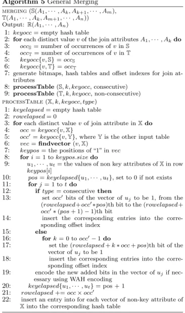
Algorithm 5General Merging

merging₍S_(A1,· · ·_{, Ak, Ak+1,}· · ·_{, Am),} T(A1,· · ·, A_k, Am+1,· · ·, An))

Output: R(A₁,· · ·, An)

1: keyocc= empty hash table

2: foreach distinct valuevof the join attributesA₁,· · ·, A_kdo

3: occ_S= number of occurrences ofvinS

4: occ_T= number of occurrences ofvinT

5: keyocc{v,S}=occ_S

6: keyocc{v,T}=occ_T

7: generate bitmaps, hash tables and offset indexes for join at-tributes

8: processTable(S, k, keyocc, consecutive)

9: processTable(T, k, keyocc, non-consecutive) processTable₍X_{, k, keyocc, type)}

1: keyelapsed= empty hash table

2: rowelapsed= 0

3: foreach distinct valuevof join attribute inXdo

4: occ=keyocc{v,X}

5: occ=keyocc{v,Y}, whereYis the other input table

6: vec=findvector(v,X)

7: keypos= the positions of “1” invec

8: fori= 1 tokeypos.sizedo

9: u1,· · ·, ut= the values of non key attributes ofXin row keypos[i]

10: pos=keyelapsed{u1,· · ·, ut}, set to 0 if not exists

11: forj= 1 totdo

12: iftype= consecutivethen

13: setocc bits of the vector ofujto be 1, from the (rowelapsed+occ∗pos)th bit to the (rowelapsed+ occ∗(pos+ 1)−1)th bit

14: insert the corresponding entries into the corre-sponding offset index

15: else

16: fork= 0 toocc−1do

17: set the (rowelapsed+k∗occ+pos)th bit of the vector ofujto be 1

18: insert the corresponding entries into the corre-sponding offset index

19: encode the new added bits in the vector ofuj if nec-essary using WAH encoding

20: keyelapsed{u1,· · ·, ut}= pos + 1

21: rowelapsed+=occ×occ

22: insert an entry into for each vector of non-key attribute of Xinto the corresponding hash table

appears twice in both SandT.

Based on this result, we can easily generate the bitmap of

Employee inR: Jones occurs 2×3 = 6 times and thus its vector is 1111110000. Ellisoccurs 2×2 = 4 times and thus its vector is 0000001111. The hash table and offset index for

Employeeare also constructed accordingly.

In the second pass, for each distinct join value, we find the value of other attributes inSandT. For values of non-key attributes inT(orS), we put them in a consecutive way and thus can correspondingly compute the positions for each value. For values of non-key attributes in S(orT), we put them in a non-consecutive way but with the same distance and thus we can also correctly compute the positions for each value.

Example 4.4. In Figure 4, we first process the attributes in table T. For employee Jones, we have three matching addresses: 425 Grant Ave,747 Industrial Wayand60 Aubin St. Since the number of occurrences ofJones inS is 2, we know that each of these addresses will appear twice inR. As we organize the values in a consecutive way, the address425

Grant Aveis put in the first two positions and thus has a bitmap vector 1100000000 in R. Similarly, 747 Industrial Wayhas vector 0011000000, and60 Aubin St 0000110000.

We then process the attributes in S. For employeeJones, we have two matching skills: TypingandShorthand. Since the number of occurrences ofJones inTis 3, we know that each of these skills will appear three times inR. As we or-ganize the values in a non-consecutive way, skillTyping is put in the 1st, 3rd and 5th positions and thus has a bitmap vector 1010100000 inR. Similarly,Shorthandhas a vector 0101010000.

Addresses and skills of employee Ellis are processed in a similar way. The offset index and hash table of each attribute is constructed according to the bit vector.

Algorithm 5 shows the general two-pass merging algorith-m. Lines 1-7 realize the first pass, and lines 8-9 the second pass by calling functionprocessTable twice to process table

TandS. We useTto illustrate theprocessTable procedure below, and the process onSis similar. For each distinct join attribute valuevinT, we first get the occurrences ofvinT asocc(line 4) and its occurrences inSas occ (line 5). We then find the positions ofvinT, denoted askeypos(lines 6-7). Functionfindvectorhas been discussed in Section 4.1. Each of these positions corresponds to a list of attribute val-ues in T,A_m+1,· · ·, A_n (line 9). For each attribute value

Ai(m+ 1≤i≤n), we construct its corresponding vector in

Rin either consecutive or non-consecutive way (lines 10-20).

5. EXPERIMENTS

In this section, we report the results of a set of experiments designed to evaluate our proposed data-level data evolution on column oriented databases. We test the efficiency and scalability in terms of time consumed for data evolution, on both real and synthetic data with large sizes.

5.1 Experimental Setup

Environment. The experiments were conducted on a machine with an AMD Athlon 64 X2 Dual Core processor of 3.0GHz and 4.0GB main memory. In our implementation we used the Windows file system, i.e., the tables in the column store are simulated by a set of files storing the columns, and did not take advantage of the buffer and disk management which is usually used in DBMSs.

Comparison System. We tested two baseline approach-es for query-level data evolution, one for row store and one for column store. For decomposition, the baseline approach for row stores scans the input table twice, as it is the min-imal cost involved in the decomposition (one scan for each query), and writes the output tables; the baseline approach for column stores scans the affected columns and output the corresponding columns in the output table. For merging, both baseline approaches scan the input tables twice (as-suming hash join is used), and writes the output table. The baseline approaches for row stores and column stores are denoted as “BR” and “BC” in the following figures, respec-tively.

We also tested two RDMBSs: a commercial row-oriented RDBMS (denoted as “C” in the figures), and an open source column oriented RDBMS (LucidDB [1], denoted as “L”). We disabled logging in C for fair comparison. We use “D” to refer to our data-level approach.

Data Set. Both synthetic data and real data are test-ed. We generated synthetic tables based on five parameter-s: number of tuples, number of distinct values in a colum-n, number of affected columns in a decomposition/merging, number of unaffected columns in a decomposition/merging, and the width of data values. The tuples in the synthetic data are randomly generated. In each set of experiments, we varied one parameter and fixed the others.

When testing decomposition and key-foreign key based merging, we generated a table R with a functional depen-dency, then we decomposed it into two tables S and T to test the decomposition and mergeS andTback to test the merging. Unless otherwise stated, tableRhas three columns (A1, A2, A3);A1is the primary key andA3 functionally de-pends onA2. Rhas 10 million tuples,A2 has 100 thousand distinct values andA3 has 10 thousand distinct values. The average width of the values in Ris 5 bytes. When testing general merging, we generated two joinable tablesSandT. Unless otherwise stated, S and T both have two columns (A1, A2) and (A2, A3), and 1 million tuples. MergingSand

T can result in as many as 2 billion tuples in the output tableR. A2 has 40 thousand distinct values. The number of distinct values of A1 andA3 are set to be half and one third of the number of distinct values ofA2, respectively.

For real data, we used a table in the patent database, which can be purchased from the United States Patent and Trademark Office. The table has 25 million tuples and nine attributes: patent number (key), name, first name, last name, address, country, state, city, zip. The total size of this table is roughly 30GB. The compressed bitmaps of all data sets in the experiment fit into main memory.

In the experiment we measure the time taken by each approach for data evolution.

5.2 Performance of Decomposition on

Synthet-ic Data

In this set of experiments we test the efficiency of decom-position for our approach, the two baseline approaches and query-level data evolution on the two RDBMSs. The test results are shown in Figure 5.3

Figure 5 shows the processing time of decomposition for all approaches with respect to different parameters. The horizontal axis in Figure 5(b) corresponds to the number of distinct values ofA2. The number of distinct value ofA3 is set to be 1/10 of that ofA2.

As we can see, the processing time of decomposition of each approach generally increases with the five parameter-s, and our data-level approach significantly outperforms the other approaches by up to several degrees of magnitude. Our approach is much faster even compared with the baseline ap-proaches, which only perform scans of the tables / columns, and writes the output tables. The processing time of our approach is mainly due to the process of building the new bitmap ofA3according to the occurrences of distinct values ofA2 inR, which is proportional to the number of distinc-t values of A2. Since the bitmap of each column is com-pressed, the size of the bitmap increases much more slowly than the number of tuples. On the other hand, table scans and writing results onto disks can take much longer time, as a column is usually much larger than its compressed bitmap. Note that BC is generally faster than BR as it does not need

3_{Some data points are missing as the corresponding}

Figure 5: Processing Time of Decomposition

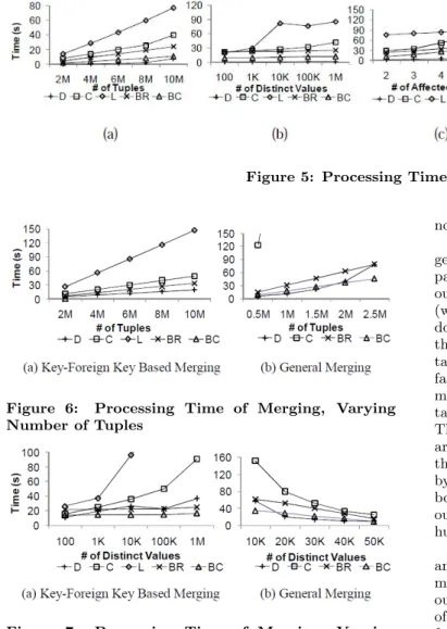
Figure 6: Processing Time of Merging, Varying

Number of Tuples

Figure 7: Processing Time of Merging, Varying

Number of Distinct Values

to scan or output the unaffected columns.

The processing time of decomposition of the two RDBMSs involves a projection query and a distinction query. C takes a relatively long time for the projection query, as the num-ber of disk I/Os is large. Since L uses bitmap indexes, it is efficient for distinction queries. However, L is generally inefficient as it takes a long time to rebuild the bitmap index after the new tables are generated.

Besides, Figure 5(d) and (e) suggest that our approach is almost not affected by increasing the number of unaffected columns, as they can be reused, and by increasing the tuple width, as the majority of our operations are on bitmaps.

5.3 Performance of Merging on Synthetic

Da-ta

In this section we report the merging processing time (in-cluding key-foreign key based merging and general merging) for these approaches. Note that we use smaller input ta-bles for general merging, but the size of the output table of general merging is comparable with the output table of key-foreign key based merging. Since L is extremely slow for both key-foreign key based merging and general merging (taking more than 12 hours for a single join query), we do

not include L in the corresponding merging test.

The processing time of key-foreign key based merging and general merging of each approach with respect to different parameters is shown in Figure 6 - Figure 8. As we can see, our approach usually outperforms the baseline approaches (which merely scans the tables and outputs the results, but do not perform any join), and is slower but comparable with the BC approach in a few cases. In fact, performing joins take a long time, indicated by the fact that our approach is far more efficient than C and L. For key-foreign key based merging, our approach scans the key attributes of the input table S once, which is the smaller of the two input tables. There are some additional bitmap “OR” operations, which are efficient for compressed bitmaps. For general merging, the processing time of the baseline approaches is dominated by the size of the output table, as it is much bigger than both input tables. On the other hand, our approach do not outputs this table, but its bitmaps, which is usually several hundred times smaller.

Our approach is far more efficient and scalable than C and L. As an example, when the number of tuples is 2.5 million, C takes almost an hour for general merging while our approach consumes only 78 seconds; when the number of affected columns is 6, C and L take 68 and 433 seconds for key-foreign key based merging, while our approach takes 33 seconds.

Note that, as can be seen from Figure 7(b), the processing time of general merging of all approaches decreases when the number of distinct values increase, as the number of tuples in the output table decreases with increasing number of distinct values. Besides, similar as decomposition, the processing time of our approach is almost not affected by the number of unaffected columns.

5.4 Performance of Decomposition and

Merg-ing on Real Data

In the patent table, attributes “first name” and “last name” functionally depend on “name”. Therefore we test a decom-position which separates these three attributes into a new table. A merging is also tested as the reverse of the decom-position. LucidDB is not included in this test due to its extremely slow speed for processing this large table.

The test shows that our approach is significantly faster than the commercial database on this data set. We take 71 and 133 seconds to perform the decomposition and merging. Contrarily, C takes 308 seconds to perform the decomposi-tion. For the merging, C does not finish in one hour, largely due to the poor scalability of C. Such a performance makes data evolution prohibitive and prevents it from being used.

0 40 80 120 160 10 20 30 40 50 Tuple Width D C L BR BC 0 20 40 60 80 100 120 2 3 4 5 6 # of Unaffected Columns D C L BR BC 0 30 60 90 120 150 2 3 4 5 6 # of Affected Columns D C L BR BC 0 30 60 90 120 100 1K 10K 100K 1M # of Distinct Values D C L BR BC 0 20 40 60 80 2M 4M 6M 8M 10M Ti m e ( s) # of Tuples D C L BR BC

(a) Key-Foreign Key (b) General (c) Key-Foreign Key (d) Key-Foreign Key (e) General

Figure 8: Processing Time of Merging, Varying Width of Values and Number of Columns

6. RELATED WORKS

Column Oriented Databases. Notable database man-agement systems that store data via columns include Mon-etDB [12], LucidDB [1] and C-Store [33]. They all support relational databases and data warehouses, on which SQL queries can be executed. C-Store additionally supports hy-brid structures of both row oriented and column oriented storages, as well as overlapping columns to speed up query processing. A detailed investigation of compression schemes on column oriented databases and guidance for choosing these schemes are presented in [5]. [19] compares the per-formance of column oriented databases and row oriented databases with respect to various factors, such as the num-ber of columns accessed by a query, L2 cache prefetching, selectivity, tuple width, etc., and demonstrates that colum-n oriecolum-nted databases are icolum-n gecolum-neral more efficiecolum-nt thacolum-n row oriented databases for answering queries that do not access many attributes. [3] studies how column stores handle wide tables and sparse data. An optimization strategy that joins columns into rows as late as possible when answering queries is presented in [7]. [4] shows that column oriented databas-es are well suitable for handling vertically partitioned RDF data, which achieves an order of magnitude improvemen-t in efficiency compared wiimprovemen-th row orienimprovemen-ted daimprovemen-tabases. [6] conducts a comprehensive study of the fundamental differ-ences between row stores and column stores during query processing, investigates whether the performance advantage of column stores can be achieved by row stores using vertical partitioning, as well as how much each optimization strate-gy affects the performance of column stores. All these works on column stores study the query processing efficiency, while data evolution on column stores has not been addressed.

Database Evolution and Related Topics. A database evolution generally involves updating the schema of the database, and evolving the data to the new schema. Existing re-search on database evolution studies procedures and effects of database schema updates. Clio [26] is a system that en-ables users to express schema mappings in terms of queries, and then uses query-level data evolution to evolve the da-ta between schemas on XML or relational dada-tabases. Oth-er works include the impact-minimizing methodology [30], propagations of the changes of applications to databases [20], consistency preservation upon schema changes [14] and frame-works of metadata model management [11, 34, 37]. Recent-ly, [15] presents the requirements of an operational tool for schema update, e.g., interface, monitoring of redundancy, query rewriting, documentation, etc., but it lacks algorithm-s that actually evolve the data from the original algorithm-schema to the new one.

Note that the data evolution problem studied in this paper

is quite different from the data migration techniques stud-ied and applstud-ied in both industry and academia. Commercial DBMSs, such as DB2, Oracle and SQL Server, provide sup-port for data migration, which is the process of migrating a database between different DBMSs. However, the database schema generally does not change during this process. Data migration is also regarded as a disk scheduling problem [22, 24, 23], which focuses on scheduling disk communication-s communication-such that a communication-set of data itemcommunication-s are trancommunication-sferred from the source disks to the target disks in minimal time. Various approximation algorithms are proposed to tackle this NP-hard problem.

Other related features supported in commercial DBMS products include the Oracle Change Management Pack [2], which provides useful operations to manage change to databas-es, e.g., it allows developers to track changes to objects as the database schema changes, and to quickly assess the impact of a database evolution and modify the relevant applications accordingly. Besides, online data reorganization in commer-cial DBMSs is a technique that enables the database to be usable when it is being maintained.

7. CONCLUSIONS AND FUTURE WORK

In this paper we present a framework for efficient data-level data evolution on column oriented databases, based on the observation that column oriented databases have a storage scheme better suitable for database evolution. Tra-ditionally, data evolutions are conducted by executing SQL queries, which we name as query level data evolution. Such a time consuming process severely limits the usability and convenience of the databases.

We exploit the characteristics of column stores and pro-pose a data-level data evolution which, instead of joining columns to form results of SQL queries and then separately compressing and storing each column, evolves the data di-rectly from compressed storage to compressed storage. Both analysis and experiments verify the plausibleness of our ap-proach and show that it consumes much less time and scales better than query level data evolution. Our approach makes databases more usable and flexible, relieves the burden of users and system administrators, and encourages research on further utilization of database evolution. This frame-work also guides the choice between row oriented databases and column oriented databases when schema changes are potentially wanted. In the future, we would like to study whether the algorithm of merging tables can be applied to optimize join queries, and the applications with excessively large tables such that the bitmap vector of a single attribute does not fit in main memory, as well as the cases in which columns are not compressed using bitmap.

8. ACKNOWLEDGEMENT

This material is based on work partially supported by NSF CAREER Award IIS-0845647, IIS-0915438 and IBM Faculty Award.

9. REFERENCES

[1] LucidDB. http://www.luciddb.org/.

[2] Oracle Enterprise Manager 10g Change Management Pack, 2005. Oracle Data Sheet.

[3] D. J. Abadi. Column Stores for Wide and Sparse Data. InCIDR, pages 292–297, 2007.

[4] D. J. Abadi, A. M. 0002, S. Madden, and K. J. Hollenbach. Scalable Semantic Web Data Management Using Vertical Partitioning. InVLDB, pages 411–422, 2007.

[5] D. J. Abadi, S. Madden, and M. Ferreira. Integrating Compression and Execution in Column-Oriented Database Systems. InSIGMOD Conference, pages 671–682, 2006.

[6] D. J. Abadi, S. Madden, and N. Hachem.

Column-Stores vs. Row-Stores: How Different Are They Really? InSIGMOD Conference, pages 967–980, 2008.

[7] D. J. Abadi, D. S. Myers, D. J. DeWitt, and S. Madden. Materialization Strategies in a

Column-Oriented DBMS. InICDE, pages 466–475, 2007.

[8] R. B. Almeida, B. Mozafari, and J. Cho. On the Evolution of Wikipedia. InICWSM, 2007.

[9] G. Antoshenkov. Byte-Aligned Bitmap Compression. InDCC, 1995.

[10] Z. Bellahsene. Schema Evolution in Data Warehouses.

Knowl. Inf. Syst., 4(3):283–304, 2002.

[11] P. A. Bernstein. Applying Model Management to Classical Meta Data Problems. InCIDR, 2003. [12] P. A. Boncz, M. Zukowski, and N. Nes.

MonetDB/X100: Hyper-Pipelining Query Execution. InCIDR, pages 225–237, 2005.

[13] Y. Chen, W. S. Spangler, J. T. Kreulen, S. Boyer, T. D. Griffin, A. Alba, A. Behal, B. He, L. Kato, A. Lelescu, C. A. Kieliszewski, X. Wu, and L. Zhang. SIMPLE: A Strategic Information Mining Platform for Licensing and Execution. InICDM Workshops, pages 270–275, 2009.

[14] A. Cleve and J.-L. Hainaut. Co-transformations in Database Applications Evolution. InGTTSE, pages 409–421, 2006.

[15] C. Curino, H. J. Moon, and C. Zaniolo. Graceful Database Schema Evolution: the PRISM Workbench.

PVLDB, 1(1):761–772, 2008.

[16] C. Curino, H. J. Moon, and C. Zaniolo. Automating Database Schema Evolution in Information System Upgrades. InHotSWUp, 2009.

[17] F. Deli`ege and T. B. Pedersen. Position List Word Aligned Hybrid: Optimizing Space and Performance for Compressed Bitmaps. InEDBT, pages 228–239, 2010.

[18] H. Fan and A. Poulovassilis. Schema Evolution in Data Warehousing Environments - A Schema Transformation-Based Approach. InER, pages 639–653, 2004.

[19] S. Harizopoulos, V. Liang, D. J. Abadi, and

S. Madden. Performance Tradeoffs in Read-Optimized Databases. InVLDB, pages 487–498, 2006.

[20] J.-M. Hick and J.-L. Hainaut. Database Application Evolution: A Transformational Approach.Data Knowl. Eng., 59(3):534–558, 2006.

[21] H. V. Jagadish, A. Chapman, A. Elkiss,

M. Jayapandian, Y. Li, A. Nandi, and C. Yu. Making database systems usable. In SIGMOD, 2007.

[22] S. Khuller, Y. A. Kim, and A. Malekian. Improved Algorithms for Data Migration. In

APPROX-RANDOM, pages 164–175, 2006.

[23] S. Khuller, Y. A. Kim, and Y.-C. J. Wan. Algorithms for Data Migration with Cloning. InPODS, pages 27–36, 2003.

[24] Y. A. Kim. Data Migration to Minimize the Total Completion Time.J. Algorithms, 55(1):42–57, 2005. [25] Z. Liu, S. Natarajan, B. He, H.-I. Hsiao, and Y. Chen.

CODS: Evolving Data Efficiently and Scalably in Column Oriented Databases. PVLDB, 3(2):1521–1524, 2010.

[26] R. J. Miller, M. A. Hern´andez, L. M. Haas, L.-L. Yan, C. T. H. Ho, R. Fagin, and L. Popa. The Clio Project: Managing Heterogeneity.SIGMOD Record,

30(1):78–83, 2001.

[27] H. J. Moon, C. Curino, A. Deutsch, C.-Y. Hou, and C. Zaniolo. Managing and Querying Transaction-time Databases under Schema Evolution.PVLDB, 1(1):882–895, 2008.

[28] P. E. O’Neil and D. Quass. Improved Query Performance with Variant Indexes. InSIGMOD Conference, pages 38–49, 1997.

[29] G. ¨Ozsoyoglu and R. T. Snodgrass. Temporal and Real-Time Databases: A Survey.IEEE Trans. Knowl. Data Eng., 7(4):513–532, 1995.

[30] Y.-G. Ra. Relational Schema Evolution for Program Independency. InCIT, pages 273–281, 2004. [31] R. Ramakrishnan and J. Gehrke.Database

Management Systems, 3rd Edition.McGraw Hill Higher Education, 2002.

[32] K. Stockinger, J. Cieslewicz, K. Wu, D. Rotem, and A. Shoshani. Using Bitmap Index for Joint Queries on Structured and Text Data, 2008.

[33] M. Stonebraker, D. J. Abadi, A. Batkin, X. Chen, M. Cherniack, M. Ferreira, E. Lau, A. Lin, S. Madden, E. J. O’Neil, P. E. O’Neil, A. Rasin, N. Tran, and S. B. Zdonik. C-Store: A Column-oriented DBMS. In

VLDB, pages 553–564, 2005.

[34] Y. Velegrakis, R. J. Miller, and L. Popa. Mapping Adaptation under Evolving Schemas. InVLDB, pages 584–595, 2003.

[35] K. Wu, E. J. Otoo, and A. Shoshani. On the Performance of Bitmap Indices for High Cardinality Attributes. InVLDB, pages 24–35, 2004.

[36] K. Wu, E. J. Otoo, and A. Shoshani. Optimizing bitmap indices with efficient compression.TODS, 31(1), 2006.

[37] C. Yu and L. Popa. Semantic Adaptation of Schema Mappings when Schemas Evolve. InVLDB, pages 1006–1017, 2005.