Department of Economics
Working Paper No. 0311
http://nt2.fas.nus.edu.sg/ecs/pub/wp/wp0311.pdf
Competing Payment Schemes
Graeme Guthrie
Victoria University of Wellington
National University of Singapore
Julian Wright
September 9, 2003
Abstract: This paper presents a model of competing payment schemes. Unlike previous work on
generic twosided markets, the model allows for the fact that in a payment system users on one
side of the market (merchants) compete to attract users on the other side (consumers who may
use cards for purchases). It analyzes how competition between card associations and between
merchants affects the choice of interchange fees, and thus the structure of fees charged to
cardholders and merchants. Implications for other two-sided markets are discussed.
© 2003 Graeme Guthrie and Julian Wright. Corresponding author: Julian Wright, Department of
Economics, Faculty of Arts and Social Sciences, National University of Singapore, AS2 Level 6, 1 Arts
Link, Singapore 117570. [email protected]. We thank seminar participants at the University of
Auckland and the University of Melbourne for helpful comments, especially Matthew Ryan. Any errors
are our own. Views expressed herein are those of the authors and do not necessarily reflect the views of
the Department of Economics, National University of Singapore.
1
Introduction
Recently several models of payment schemes have been developed in order to analyze the optimal structure of fees in debit and credit card schemes. They ask the question: How much is charged to cardholders versus merchants for card transactions? Policymakers in a number of jurisdictions have been concerned that merchants pay too much to accept credit card transactions, costs that in their view are ultimately covered by consumers who pay by other means (see Chang and Evans, 2000, and Chakravorti and Shah, 2003).
The optimal structure of cardholder and merchant fees was first addressed by Baxter (1983), who viewed a payment transaction as ajoint service consumed by cardholders and merchants. He emphasized the importance of a structure of fees for which cards are used whenever their joint transactional benefits exceed their joint costs. Baxter’s was a normative analysis. Schmalensee (2002) and Rochet and Tirole (2002) have since provided positive analyses, explaining what determines the structure of fees set by a payment card association (such as MasterCard or Visa). While Schmalensee focuses on the trade-off between attracting cardholders and attracting merchants, Rochet and Tirole analyze a corner solution in which all merchants accept cards in equilibrium. A key feature of Rochet and Tirole’s model is that they derive consumer and merchant demand from first principles, allowing for the fact merchants compete to attract customers (some of whom may be cardholders). Wright (2003a) combines elements of both approaches to explore the sources of divergence between the privately and socially optimal fee structures. However, all of these authors assume there is justonepayment system that is choosing its price structure.1
This paper relaxes this assumption.
In considering how competition between payment schemes determines the structure of fees between cardholders and merchants, this paper also falls within the recent literature on two-sided markets. These markets have the property that there are two types of agents that wish to use a common platform, and the benefits of each side depend on how many users there are on the other side of the network. Rochet and Tirole (2003) provide a general model of platform competition in a two-sided market. Examples they give include Adobe Acrobat (Acrobat Reader and Writer), payment cards (cardholders and merchants), platforms (hardware/console and software providers), real estate (home buyers and sellers), shopping malls (shoppers and retailers), and Yellow Pages (readers and advertisers). In contrast to their model of a single payment scheme (Rochet and Tirole, 2002), they treat users on both sides as end users, abstracting from the fact that an important feature of some of these markets is that one side competes amongst itself to sell to the other side (e.g. merchants, software providers, home sellers, retailers and advertisers).2 In contrast, we allow for competition between merchants (sellers)
In addition to allowing for competition between merchants and competition between schemes, we also allow for consumers to make separate card-holding and card-usage decision. Our main analysis is presented in terms of a model of two competing card associations, such as MasterCard and Visa. For such schemes the structure of cardholder and merchant fees is determined by the level of the interchange fee, a fee set collectively by the members of the associations. The interchange fee is paid by the merchant’s bank to the cardholder’s bank on each card transaction. A higher interchange fee results in higher merchant fees and lower card fees. We model how the two types of competition alter the equilibrium interchange fee, and compare this to the socially optimal level. To obtain sharp results, we focus on the benchmark case
1
This is also true of other recent models in the literature including Chakravorti and To (2000), Gans and King (2003), Schwartz and Vincent (2002), Wright (2003b), and Wright (2003c). Rochet and Tirole (2002) do discuss the impact of scheme competition in their model, but they do not find the resulting equilibrium.
2
Other papers that model two-sided markets also abstract from the strategic interaction between sellers. These include Armstrong (2002), Caillaud and Jullien (2001, 2003), Parker and Van Alstyne (2000), and Schiff (2003).
in which consumers view the two types of cards as providing identical transactional benefits for making purchases, and merchants view the two types of cards as providing identical transactional benefits for receiving payment.
To compare results from our model with those of Rochet and Tirole (2002), we start with the bench-mark case in which there is only a single card scheme, before allowing for competition between schemes in which consumers choose whether to hold none, one or both cards, and merchants choose whether to accept none, one or both cards. To see how merchant competition matters, in each case we start with a model in which the merchant is a monopolist, and so does not use card acceptance as a strategic instrument of competition. We then consider what happens when merchants compete in a Hotelling fashion.
A key determinant of the competitive fee structure (and interchange fee) is the extent to which con-sumers hold one or two cards when making purchases. With both forms of merchant behavior considered, when consumers only choose to hold one card, competition between card schemes does not result in lower interchange fees. In this case, by attracting cardholders, card schemes have a monopoly over access to these cardholders. This leads competing card schemes to care only about the surplus they can offer to cardholders, leaving no surplus to merchants (the case of a competitive bottleneck).
This competitive bottleneck outcome can be undermined provided some consumers hold both cards. Then the unique equilibrium in our model involves competing card schemes seeking to attract merchants exclusively, by offering maximal incentive for merchants to accept their cards. In the case of monopolistic merchants, this implies maximizing the expected surplus offered to merchants. In the case of competing merchants, this involves maximizing the expected joint surplus of consumers and merchants, given that competing merchants take into account the benefits that their customers get from being able to use cards. In either case, interchange fees are lower to the extent there is competition between schemes, but higher to the extent there is competition between merchants. When the two effects are combined, so there is competition between schemes and between merchants, the equilibrium interchange fee remains inefficiently low, but only to the extent that issuers and acquirers obtain positive margins.
The rest of the paper proceeds as follows. In Section 2 we present our model, starting with the case of a single card scheme. Section 3 considers the case of two identical competing payment card associations. Section 4 considers several extensions and implications of our analysis. Section 4.1 shows that our results also hold for the case of competing proprietary schemes, like American Express and Discover card, that set their cardholder and merchant fees directly. Section 4.2 considers how our results extend to allow for merchant heterogeneity. Section 4.3 explains how the existence of some cash-constrained consumers alters the equilibrium fee structure. Implications for policy and for the analysis of other two-sided markets are discussed in Sections 4.4 and 4.5. Finally, Section 5 provides some concluding remarks.
2
A single card scheme
We start by considering the simpler case of a single payment scheme where the only alternative to using cards is cash, before introducing competing payment schemes in the next section. This allows some of the analysis we will use in the next section to be first developed in a simpler setting. It also allows our model to be compared to the framework of Rochet and Tirole (2002) in the case in which there is only a single payment scheme. In addition to considering strategic merchants, as they do, we also allow for the case of monopolistic merchants, and for consumers to make separate joining and card usage decisions. Another difference between our model and theirs is that in our model consumers are assumed to receive their particular draw of transactional benefits from using cards once they have chosen which merchant
to purchase from.
In the model of Rochet and Tirole, consumers get their draw of transactional benefits before they choose which merchant to purchase from. Clearly our timing assumption is made for modelling conve-nience. We think it is a reasonable modelling approach for two reasons. First, with our set-up, consumers still choose which merchant to purchase from (in the case of competing merchants) taking into account the expected benefits from using cards versus the alternative payment instrument. By accepting cards, merchants will raise consumers’ expected benefit from purchasing from them, since consumers will gain the option of using cards for purchases. In fact, this section shows the timing assumption does not alter the equilibrium conditions under which merchants accept cards or consumers use cards: they are equiv-alent to the condition derived in Rochet and Tirole (2002) and Wright (2003a) for a Hotelling model of merchant competition, and to the condition derived in Baxter (1983) and Wright (2003c) in the case of monopolistic merchants. Thus, we do not think this particular timing assumption is driving the results we obtain. Additionally, the timing assumption can be motivated by the idea that consumers only learn of their particular need to use various types of payments once they are in the store.
A card association represents the joint interests of its members, who are issuers (banks and other financial institutions which specialize in servicing cardholders) and acquirers (banks and other financial institutions which specialize in servicing merchants). In such an open scheme, a card association sets an interchange feeato maximize its members’ collective profits.3 The interchange fee is defined as an amount
paid from acquirers to issuers per card transaction. In addition, we assume a cost ofcI per transaction
of issuing andcA per transaction of acquiring. A proprietary scheme incurs the cost cI +cA of a card
transaction. Competition between symmetric issuers and competition between symmetric acquirers then determines the equilibrium fee per transaction for using cards,f, and the equilibrium fee per transaction for accepting cards,m. In the case of a proprietary card scheme such as American Express, the scheme setsf andmdirectly to maximize its profits.
We follow Rochet and Tirole (2003, Section 6.2) and make the simplifying assumption that competition between symmetric issuers and between symmetric acquirers leaves some small constant equilibrium margin to issuers and to acquirers, so that
f(a) =cI−a+πI (1)
whereπI is some small constant profit margin.4 Likewise, merchant fees are
m(a) =cA+a+πA, (2)
where πA is some small constant profit margin. Intense intra-platform competition results in (as a first
order approximation) the number of card transactions being taken as given, so that symmetric Hotelling or Salop style competition between banks would lead to the above equilibrium fees.
Card fees can be negative to reflect rebates and interest-free benefits offered to cardholders based on their card usage. Card fees decrease and merchant fees increase as the interchange fee is raised. The implication of the above assumption about bank competition is that the level of the interchange fee affects only the structure of fees, and not the overall level of fees: the sum of cardholder and merchant fees per-transaction, denoted by l = f(a) +m(a), is independent of the interchange fee a (it equals
3In our set-up below this is also equivalent to assuming that the card association seeks to maximize the total number of card transactions. Notably, MasterCard and Visa (the card associations) obtain revenues from a small levy on each card transaction collected from their members, so they would seem to have the same incentives as their members.
cA+cI +πA+πI). As a result, a card association will maximize its members’ profits by choosing its
interchange fee to maximize its volume of card transactions.
As in Rochet and Tirole (2002), consumers get transactional or convenience benefits bB from using
cards as opposed to the alternative cash, and merchants get transactional or convenience benefits bS
from accepting cards relative to the alternative of accepting cash. The benefits bB are drawn with a
positive densityh(bB) over the interval [bB, bB]. The hazard functionh(f)/(1−H(f)) is assumed to be
increasing, where H denotes the cumulative distribution function corresponding to bB. All merchants
(sellers) are assumed to receive the same transactional benefitsbS from accepting cards (this assumption
will be relaxed later). We will refer tobB−f as the ‘surplus’ to consumers from using cards, andbS−m
as the ‘surplus’ to merchants from accepting cards. (Note, however, if merchants compete to attract cardholders, they will also profit from accepting cards through a business stealing effect.) We assume that
E(bB) +bS < l < bB+bS (3)
so as to rule out the possibility that there is no card use and to rule out the possibility that all consumers use cards.
It costs merchants dto produce each good, and all goods are valued at v by all consumers. There is a measure 1 of consumers who wish to buy from merchants. Consumers are assumed to each want to purchase one good. We also assume
v−d≥l−bB−bS+
1−H(bB)
h(bB) ,
which is used in Appendix B to show that even monopolistic merchants will set a price such that consumers who pay by cash will still want to purchase. Throughout, merchants are assumed to be unable to price discriminate depending on whether consumers use cards or not, so consumers will want to pay with the card if and only if bB ≥f.5 Using this property, we can define a number of important functions. The
quasi-demand for card usage is defined as D(f) = 1−H(f), which is the proportion of consumers who want to use cards at the fee f. The average convenience benefit to those consumers using cards for a transaction isβ(f) =E[bB|bB ≥f], which is increasing inf. The expected surplus to a consumer (buyer)
from being able to use their card at a merchant is
φB(f) =D(f) (β(f)−f), (4)
which is positive and decreasing inf. The expected surplus to a merchant (seller) from being able to accept cards isD(f)(bS−m), which, given that f+m=l, can be defined as
φS(f) =D(f) (f+bS−l). (5)
Finally, the expected joint surplus to consumers and merchants from card usage is defined as
φ(f) =D(f)(β(f) +bS−l), (6)
which equalsφB(f) +φS(f).
The following lemma summarizes some useful properties of these functions, and introduces three important levels of the interchange fee.
5This no price discrimination assumption can be motivated by the no-surcharge rules that card associations have adopted to prevent merchants from charging more to consumers for purchases made with cards. It can also be motivated by the observation of price coherence (Frankel, 1998) — that merchants are generally reluctant to set differential prices depending on the payment instrument used.
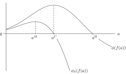
Figure 1: Important interchange fees
0 a
aM aC aΠ
φ(f(a))
φS(f(a))
Notes. The interchange feeaM maximizesφ
S(f(a)), the expected surplus to a merchant from being able to
accept cards, whileaCmaximizesφ(f(a)), the expected joint surplus to consumers and merchants from card
usage. φS(f(a)) = 0 at the interchange feeaC, whileφ(f(a)) = 0 ataΠ.
Lemma 1
1. There exists a unique interchange fee, denotedaC, which maximizes φ(f(a)). It equals
aC=bS−cA−πA (7)
and is the unique interchange fee which solves φS(f(a)) = 0.
2. There exists a unique interchange fee, denotedaM, which maximizesφ
S(f(a)).
3. There exists a unique interchange fee, denotedaΠ, which solves φ(f(a)) = 0.
4. The interchange feesaC,aM, andaΠ satisfyaM < aC < aΠ.
Proof. See Appendix A.1. ¥
The results of this lemma are summarized in Figure 1.
Each consumer enjoys some intrinsic benefit,u, from holding a card, which is a random variable with positive density e over the interval (−∞, u] for some u≥ 0. We let A(u) = 1−E(u), where E is the cumulative distribution function foru. For some consumersu <0, so that holding a card (which is not used) is inconvenient. This could also represent the case that there are some costs to issuers associated with managing a cardholder, if these costs are fully passed through to cardholders. For other consumers, cards offer more than just the ability to make transactions at merchants (for example, they may be used as security or to withdraw cash), in which caseu >0. The variableλcaptures the measure of consumers who choose to hold a card.
The timing of the game is summarized as follows:
(i). The payment card association sets the level of its interchange feea. Issuers and acquirers then set feesf andm to cardholders and merchants according to (1) and (2). Alternatively, a proprietary scheme sets f andmdirectly.
(ii). Consumers get their draw of u and decide whether or not to hold the card. Merchants decide whether or not to accept the card.
(iii). Merchants set their retail prices. If relevant, consumers decide which merchant to buy from. (iv). Based on their individual realizations ofbB, consumers decide whether to use the card for payment
(if they hold the card), or cash.
We first start with the case of monopolistic merchants.
2.1
Monopolistic merchants
By considering monopolistic merchants, we abstract from the business stealing motive that can influence a merchant’s card acceptance strategy. This non-strategic approach is the setting that underlies the seminal analysis of Baxter (1983), in which he considered a merchant that accepted cards whenever the transactional benefits it obtained from doing so exceeded the merchant fee it was charged.
The following lemma describes the possible equilibria in stage (ii) of the game, and shows the Baxter condition for card acceptance also applies here.
Lemma 2 Suppose a single card scheme has a card fee off. IfφS(f)<0, then monopolistic merchants
reject the card and λ(f) = A(0) consumers hold the card. If φS(f) ≥0, then monopolistic merchants
accept the card, andλ(f) =A(−φB(f))consumers hold the card.
Proof. We solve the game by working backwards through the stages. The stages are described in turn. Stage (iv).
If consumers hold a card, they will use the card if bB ≥f and the merchant they buy from accepts
the card and sets a pricep≤v. If consumers hold a card, they will use the card ifbB ≥f+p−vand the
merchant they buy from accepts the card and sets a pricep > v. In any other circumstance, consumers will not use a card.
Stage (iii).
Provided it sets its price no higher than v, a merchant obtains profit of
π=p−d+λ(f)D(f) (bS−m)I,
whereIis an indicator variable which takes the value 1 if the merchant accepts the card and 0 otherwise. Alternatively, a merchant can setp > v, in which case it will only sell to cardholders who use cards, so that
π=λ(f)D(f+p−v) (p−d+bS−m)I.
As we prove in Appendix B, it will not be profitable for a merchant to set a price abovev, and exclude ‘cash customers’ (both those who do not hold a card and those who do not wish to use a card), provided the surplus from the good itself is sufficiently large. Instead, a monopolist will extract all the surplus from the cash customers by settingp=v, implying it earns a profit of
π=v−d+λ(f)φS(f)I.
Stage (ii).
Given a merchant obtains a price of v regardless of whether it accepts cards or not, it will accept cards if and only ifφS(f)≥0. A consumer’s benefit from holding the card is thenφB(f)I+u. It follows
that consumers will hold a card ifu > 0 and φS(f)<0 (using it only to withdraw cash and the like).
They will also hold a card ifu >−φB(f) andφS(f)≥0. If neither condition applies, consumers will not
hold a card. The equilibria in stage (ii) are thus those characterized by the lemma. ¥
The card scheme’s profit (that is, the total profit of the association’s member banks) is zero ifφS(f)<
0, since merchants will not accept cards, and is equal to
Π(f) = (πA+πI)A(−φB(f))D(f)
ifφS(f)≥0. Then we have
Proposition 1 Facing monopolistic merchants, a single card scheme sets its interchange fee to solve
φS(f) = 0; that is, ata=aC.
Proof. A single card association maximizes Π(f) by choosingf to maximizeA(−φB(f))D(f) subject to
the constraintφS(f)≥0 which ensures merchants accept cards. The constraint is equivalent tof+bS ≥l.
SinceA(−φB(f))D(f) is decreasing inf and the left hand side of the constraint is increasing inf, this
implies the scheme will wish to setf as low as possible subject to the constraint. The constraint will be binding and the profit maximizing interchange fee solves φS(f) = 0, which from Lemma 1 is precisely
the interchange feeaC defined in (7). ¥
The single card scheme sets an interchange fee which leaves merchants with no surplus from accepting cards. This occurs when the fee charged to merchants equals the transactional benefits they obtain. This is also the (constrained) socially optimal level of the interchange fee, given monopolistic merchants. We have:
Proposition 2 Facing monopolistic merchants, the welfare-maximizing interchange fee isa=aC.
Proof. See Appendix A.2. ¥
Although the unconstrained socially optimal interchange fee is higher thanaC (it isb
S−cA+πI, so
that consumers use cards wheneverbB+bS > cI+cA), merchants will not accept cards if the interchange
fee is set aboveaC. The reason the interchange fee is too low here is that, facing stiff merchant resistance
to accepting cards, the card scheme is unable to get merchants to absorb the issuers’ and acquirers’ margins. Instead, consumers who use cards will cover all of these margins, which leads to under-usage of cards. The fact that some consumers can still get utility from holding cards (even if they cannot use them) does not affect this conclusion, since these consumers still get the same utility fromholding cards in the case they are able to use them.
In the limiting case of πA =πI →0, the profit maximizing interchange feeaC equal bS −cA, which
is also the Baxter interchange fee and the unconstrained socially optimal interchange fee.
2.2
Strategic merchants
In this section merchants may accept cards for strategic reasons, so as to attract customers from each other. Like Rochet and Tirole (2002), we model this by assuming there are two merchants who compete in a Hotelling fashion. In particular, consumers are uniformly distributed on the unit interval and the two merchants are located at either extreme. A consumer located atxfaces linear transportation costs oftx
from purchasing from merchant 1 andt(1−x) from purchasing from merchant 2. These transportation costs can be summarized by the function Ti(x) =tx(2−i) +t(1−x) (i−1), where i= 1 corresponds
to merchant 1 andi= 2 corresponds to merchant 2. Note that the draws ofu,x, andbBare all assumed
The following lemma describes the possible equilibria in stage (ii) of the game.
Lemma 3 Suppose a single card scheme has a card fee of f. If φ(f) < 0, then competing merchants reject the card andλ(f) =A(0) consumers hold the card. Ifφ(f)≥0, then competing merchants accept the card andλ(f) =A(−φB(f))consumers hold the card.
Proof. We solve the game by working backwards through time. The steps are described in turn. Stage (iv).
Since consumers face the same price whether paying by card or by cash, they will only use the card ifbB ≥f and the merchant they buy from accepts the card.
Stage (iii).
When deciding which merchant to buy from, consumers take into account their location in product space (their exogenous preference for the two merchants), whether or not they hold a card, the price charged by each merchant, and whether or not the merchants accept the card. A consumer located atx
who buys from merchantiobtains indirect utility equal to
vi=v−pi−Ti(x)
if they do not hold a card, and equal to
vi=v−pi+φB(f)Ii−Ti(x)
if they hold the card, whereIi is an indicator variable which takes the value 1 if merchantiaccepts the
card and 0 otherwise. The share of customers that firm 1 will attract is therefore
s1=
1 2 +
1
2t(p2−p1+λ(f)φB(f) (I1−I2)), (8)
whereλ(f) equals the measure of consumers holding cards given the card feef. Firm 2 attracts a share
s2= 1−s1 of consumers. Merchanti’s profit is
πi=si(pi−d−λ(f)D(f) (m−bS)Ii). (9)
We solve for the Nash equilibrium in this stage by working out each merchant’s profit-maximizing choice of prices given the share function (8). Solving these best responses simultaneously shows that the equilibrium prices are p1 = t+d+λ(f)D(f)I1(m−bS) + 1 3λ(f)φ(f) (I1−I2), (10) p2 = t+d+λ(f)D(f)I2(m−bS) + 1 3λ(f)φ(f) (I2−I1). (11) Substituting (10) and (11) into (8) and (9) shows that firmiearns an equilibrium profit of
πi= 2ts2i, (12) where s1= 1 2 + 1 6tλ(f)φ(f) (I1−I2) (13) ands2= 1−s1. Stage (ii).
In this stage we determine equilibria in the subgame as simultaneous solutions of each party’s best response, conditional on the card fee and merchant fee set by the card scheme in stage (i).
Merchants’ best responses.
To work out merchants’ optimal card acceptance policy we note that, regardless of what the other merchant does, each merchant will accept cards if doing so increases its equilibrium market share. Thus, each merchant will accept cards if doing so increases the functionλ(f)φ(f), where the subscript for each merchant has been dropped since the function is the same for both merchants. Note that here merchants’ card acceptance policy is determined by φ in the same way as it was determined by φS in Lemma 2.
Thus, following the identical proof of Lemma 2 but replacingφS withφ, we end up with exactly the same
results for merchant card acceptance, except withφS replaced byφ.
Consumers’ best responses.
Their choice of card-holding depends on the benefits they get from holding a card, which depend on merchants’ acceptance decisions. Given merchants are symmetric, the above result implies either both merchants will accept cards, ifφ(f)≥0, or both merchants will reject cards. In this case we can define
I=I1=I2. A consumer’s additional benefit of holding the card is thenφB(f)I+u. If merchants reject
the card (which happens when φ(f) <0), then consumers will hold the card if and only if u ≥ 0. If merchants accept the card (which happens when φ(f)≥ 0), then consumers will hold the card if and only ifu≥ −φB(f). The equilibria in stage (ii) are thus those characterized by the lemma. ¥
Notice from the proof above that card acceptance (that is, Ii= 1) does three things. First, it raises
the demand faced by merchant i. It provides consumers with a valuable option from shopping at the merchant concerned, which is that they can use cards if doing so is convenient for them (bB > f). The
expected value of this option is measured by the term λ(f)φB(f) in the firm’s market share equation
(8). Second, and by symmetry, it lowers the demand faced by the rival firm. Thus, in this model card acceptance has a business stealing effect. Third, as the firm’s profit equation (9) reveals, card acceptance changes the merchant’s costs, increasing them ifm > bS for the merchant concerned.
We are now ready to characterize equilibrium fee structures at stage (i) of the game. We consider the profit-maximizing interchange fee. The card scheme’s profit is zero if φ(f)<0, since no merchants will accept cards, and equal to
Π(f) = (πA+πI)A(−φB(f))D(f)
ifφ(f)≥0. We have:
Proposition 3 Facing competing merchants, a single card scheme sets its interchange fee equal to aΠ,
so that φ(f(a)) = 0; that is, such that
β(f(aΠ)) +bS =l. (14)
Proof. Since πA+πI > 0, a single card association maximizes Π(f) by maximizing A(−φB(f))D(f)
subject to the constraint φ(f) ≥0 which ensures merchants accept cards. The constraint is equivalent toβ(f) +bS ≥l. Since A(−φB(f))D(f) is decreasing inf andβ(f) is increasing in f, this implies that
the card scheme’s profit is maximized by setting f = fΠ, where β(fΠ) +b
S = l and φ(fΠ) = 0. The
existence and uniqueness of the corresponding interchange feeaΠ was proven in Lemma 1. ¥
Condition (14) defines the merchant transactional benefits bS, below which both merchants will not
accept cards and above which both merchants will accept cards. Interestingly, this is the same equilibrium condition that Rochet and Tirole (2002) and Wright (2003a) obtained.6 A single card scheme sets a
6
To be precise, in Rochet and Tirole’s model the termlon the right hand side is replaced bym. This difference only arises because in their model the consumers’ feef is effectively a fixed fee and so occurs regardless of the extent to which the card is used. Moreover, Rochet and Tirole also found another equilibrium was possible in which merchants with values ofbS slightly above this critical level both reject cards, although they rule out this second equilibrium. In their model,
fee structure which encourages maximal use of cards by consumers while ensuring merchants have just enough surplus so that they will accept cards. Since merchants compete amongst themselves, they take into account their customers’ average surplus from using cards in deciding whether to accept cards or not. Thus, when the card scheme leaves merchants just indifferent between accepting cards or not, it implies that the expected joint surplus to consumers and merchants from the card scheme are exactly zero.
As in Rochet and Tirole (2002), the welfare-maximizing interchange fee is either the same as the privately chosen interchange fee set by a single scheme, or is lower.
Proposition 4 Facing competing merchants, the welfare-maximizing interchange fee is
aW = min©
bS−cA+πI, aΠª. (15)
Proof. See Appendix A.3. ¥
The unconstrained socially optimal interchange fee is the one at which consumers face the joint costs of using cards less the transactional benefits that merchants obtain. This requires a card fee of
f =cA+cI−bS. Since at this card fee consumers face the full social costs and benefits of their
card-holding decision, including the cost or benefit (u) simply from holding the card, there is no reason to distort card fees in this model to encourage or discourage additional card-holding. The only reason then to set a lower interchange fee is if this interchange fee implies merchants fees above which merchants would accept cards. It is never optimal to exclude merchants and so get no card transactions.
3
Competition between identical card schemes
We modify the model of Section 2 by assuming there are two competing identical card systems. Identical systems not only have the same costs and issuer and acquirer margins, they also provide the same benefits to cardholders and merchants. The only distinguishing feature of each card scheme is the fee structure it chooses. Specifically, each card associationisets an interchange fee denotedai.
Like the case with a single scheme, we follow Rochet and Tirole (2003, Section 6.2)7and assume that
for competing card associations
fi(ai) =cI−ai+πI (16)
and
mi(ai) =c
A+ai+πA, (17)
so that the interchange fee determines the structure but not the overall level of fees. Taking the limit of the equilibrium fee structure asπI andπA tend to zero allows us to capture the case of perfect
intra-system competition.8 As before, we definel as the sum off andm, which, from the fact that the issuers
and acquirers in each scheme are assumed to have the same costs and margins, does not depend on i. We also defineDi=D¡
fi¢
, φi
B =φB¡fi¢,φiS =φS¡fi¢, andφi=φ¡fi¢.
each firm’s acceptance decision is affected by what the other firm does. Due to our different timing assumption, each firm’s acceptance decision is independent of what other firms are doing, and so we get a unique equilibrium.
7See also Hausmanet al. (2003). 8
Like Rochet and Tirole (2003) we do not deal with issues of duality, in which banks may be members of both card associations. See Hausmanet al. (2003) for an analysis of duality. A further justification for this form of bank fees is that it can be used to recover the equilibrium fees that result from competition between two identical proprietary schemes, that set their fees directly to consumers and merchants. Section 4.1 carries out this exercise.
In stage (ii) consumers make their card-holding decision, which is now whether to hold none, one or both cards. Likewise, in stage (ii) merchants now have to decide whether to accept none, one or both cards. We letλi be the measure of consumers who hold cardi only (singlehoming consumers), andλ12
be the measure of consumers who hold both cards (multihoming consumers).
We make use of two tie-breaking conventions. First, we assume if consumers are indifferent about holding one card or another, they will randomize to determine which card to hold. Second, we assume that if merchants are indifferent between accepting a card or not because they do not expect consumers to use the card, they will accept the card if doing so would increase their profits (or at least not decrease their profits) if some consumers did use the card.
The timing of the game is summarized as follows:
(i). Each payment card association sets the level of their interchange fee ai. Issuers and acquirers
then set fees fi andmi to cardholders and merchants according to (16) and (17). Alternatively, a
proprietary schemeisetsfi andmidirectly.
(ii). Consumers decide which cards to hold (neither, one or both). Merchants decide whether to accept cards (neither, one or both).
(iii). Merchants set their retail prices. If relevant, consumers decide which merchant to buy from. (iv). Based on their individual realizations of bB, consumers decide whether to use cards or cash for
payment.
We start again with the case of monopolistic merchants, which, like the analysis of Rochet and Tirole (2003), allows competition in two-sided markets to be analyzed without considering the strategic interaction between sellers. Unlike Rochet and Tirole’s analysis of this problem, we first consider the consumers’ decisions about whether to hold none, one, or both cards, and assume all merchants get the same benefits from accepting cards.9
3.1
Monopolistic merchants
The following lemma describes the possible equilibria in stage (ii) of the game for any given card fees set by the schemes in stage (i).
Lemma 4 Suppose two identical card schemes compete, with card schemes1 and2 having card fees f1
andf2 respectively.
1. If f1 =f2 then φ1
S =φ2S and there are two cases to consider. If φ1S =φ2S ≥0, then monopolistic
merchants accept both cards and the singlehoming consumers will randomize over which card to hold. Ifφ1
S =φ2S <0, then monopolistic merchants reject both cards and there are no singlehoming
consumers.
2. Iffi< fj then four equilibria are possible at stage (ii). Ifφi S, φ
j
S <0, then monopolistic merchants
reject both cards and there are no singlehoming consumers. Ifφi S, φ j S ≥0and(λi+λ 12)φi S ≥λ12φ j S,
then monopolistic merchants accept both cards and the singlehoming consumers will only hold cardi. If φi
S≥0,φ j
S <0, then monopolistic merchants only accept cardiand the singlehoming consumers
9In Section 4.2, we consider a case in which all consumers hold both cards and merchants are heterogenous, a case closer to theirs.
will only hold cardi. IfφjS ≥0 andφi
S <0then monopolistic merchants only accept cardj and the
singlehoming consumers will only hold cardj. (Ifu >0, then this equilibrium occurs more generally if φjS ≥0 andφi
S < φ j S.)
Proof. We solve the game by working backwards through time. Stage (iv).
To characterize consumers’ usage of cards, it is useful to introduce another indicator variable, Lji,
which captures the likelihood that, assuming they get a sufficiently high draw of bB (that isbB ≥fj),
consumers who hold both cards will prefer to use cards from scheme j at merchanti. For the case of monopolistic merchants, the subscriptiis redundant. We retain it here since it will become relevant for the case of competing merchants considered in the next section. Iff1< f2 consumers will prefer to use
card 1 if merchants accept both cards (or just card 1), and will prefer to use card 2 if this is the only card accepted. We thus define
L1i =Ii1 andL2i =Ii2
¡
1−Ii1
¢
(18) iff1 < f2. Iff1 > f2 consumers will prefer to use card 2 if merchants accept both cards (or just card
2), and will prefer to use card 1 if this is the only card accepted. We thus define
L1i =Ii1¡
1−Ii2¢
andL2i =Ii2 (19)
iff1 > f2. If f1=f2 consumers will be indifferent about which card to use if merchants accept both, and so will randomize over card usage. If merchants only accept one card, then consumers prefer to use this card. We thus define
L1i =Ii1 µ 1−1 2I 2 i ¶ andL2i =Ii2 µ 1−1 2I 1 i ¶ (20) iff1=f2.
Provided merchants set their common pricepno higher thanv, consumers will only use a card if the transactional benefits of doing so are at least as high as the fee they face. If consumers only hold card
i, they will only use the card if bB ≥ fi and the merchant they buy from accepts the card. The card
use of consumers who hold both cards and drawbB ≥min{f1, f2} is described by equations (18), (19)
and (20). Alternatively, if merchants set their price abovev, then if consumers only hold cardi, they will only use the card ifbB+v≥fi+pand the merchant they buy from accepts the card. The card use of
consumers who hold both cards and drawbB ≥min{f1, f2}+p−v is described by equations (18), (19)
and (20). Stage (iii).
Given there is a measure 1 of potential consumers, provided a merchant sets its price less than or equal tovin stage (iii), the merchant’s profit is
π=p−d−λ1D1¡
m1−bS¢I1−λ2D2¡m2−bS¢I2−λ12¡D1¡m1−bS¢I1L1+D2¡m2−bS¢I2L2¢.
Alternatively, a merchant can setp > v, in which case the merchant will only sell to cardholders who use cards, so that π = λ1D¡ f1+p−v¢ ¡ p−d+bS−m1 ¢ I1+λ2D¡ f2+p−v¢ ¡ p−d+bS−m2 ¢ I2 +λ12¡¡ f1+p−v¢ ¡ p−d+bS−m1 ¢ I1L1+D¡ f2+p−v¢ ¡ p−d+bS−m2 ¢ I2L2¢ .
As we show in Appendix B, it will not be profitable for merchants to set a price abovev, and exclude ‘cash customers’ (both those who do not hold a card and those who do not wish to use a card), provided
the surplus from the good itself is sufficiently large. Instead, merchants will extract all the surplus from the cash customers by settingp=v, implying merchants earn a profit of
π=v−d+ Ψ, (21) where Ψ =λ1φ1SI1+λ2φ2SI2+λ12¡ φ1SI1L1+φ2SI2L2¢ . (22) Stage (ii).
In this stage we determine equilibria in the subgame as simultaneous solutions of each party’s best response, conditional on the card fees and merchant fees set by the two card schemes in stage (i).
The merchant’s best response.
To work out a merchant’s optimal card acceptance policy we note that a merchant will accept cards if doing so increases the function Ψ.
We must consider two possibilities for consumers’ card-holding. In the first possibility we consider, no consumers multihome, so thatλ12= 0 and the function Ψ is determined by the following table:
I2= 0 I2= 1
I1= 0 0 λ2φ2
S
I1= 1 λ1φ1
S λ1φ1S+λ2φ2S
Recall that if a merchant is indifferent between accepting and rejecting cardibecause it does not expect consumers to use cardi(so that accepting the card leaves the function Ψ unchanged), it will accept the card if doing so increases Ψ when consumers do use cardi. This is true if and only ifφi
S ≥0. Merchants
therefore adopt the following policy: merchants reject both cards if φ1
S, φ2S < 0, accept both cards if
φ1
S, φ2S ≥0, and accept only card 1 (respectively, card 2) if φ1S ≥0 > φ2S (respectively, φ2S ≥0 > φ1S).
When all consumers hold at most one card, even though there are two card schemes, the condition that determines whether merchants accept cards is identical to the case with a single card scheme. Each individual merchant does not expect to be able to influence the number of cardholders of each type, and so it acts as though these are two segmented groups of consumers.
The second possibility is that some consumers hold both cards, so that λ12>0. SinceL1 and L2 in
equation (22) depend on the values off1 andf2, we need to consider three different cases.
• Iff1=f2then φ
S =φ1S =φ2S and equation (20) implies that
Ψ =φS
¡
λ1I1+λ2I2+λ12¡
I1+I2−I1I2¢¢
.
In this case the function Ψ is determined by the following table:
I2= 0 I2= 1 I1= 0 0 ¡ λ2+λ12¢ φS I1= 1 ¡ λ1+λ12¢ φS ¡ λ1+λ2+λ12¢ φS
Merchants’ best response is to reject both cards ifφS <0 and to accept both cards ifφS ≥0.
• Iff1< f2, then equation (18) implies that
Ψ =λ1φ1 SI1+λ2φ2SI2+λ12 ¡ φ1 SI1+φ2SI2 ¡ 1−I1¢¢ .
In this case the function Ψ is determined by the following table: I2= 0 I2= 1 I1= 0 0 ¡ λ2+λ12¢ φ2 S I1= 1 ¡ λ1+λ12¢ φ1 S ¡ λ1+λ12¢ φ1 S+λ2φ2S
Merchants’ best response is as follows: merchants reject both cards ifφ1
S, φ2S<0; they accept only
card 1 if φ2
S < 0 ≤ φ1S; they accept only card 2 if φ2S ≥0 and λ12φ2S >(λ1+λ12)φ1S; and they
accept both cards if (λ1+λ12)φ1
S≥λ12φ2S ≥0.10
• Exploiting the symmetry with the above case, merchants’ best response is the same except the superscripts 1 and 2 are swapped.
Consumers’ best responses.
At stage (ii), consumers decide which card(s) to hold, if any. Their choice of card-holding depends on the benefits they get from holding a card, which depend on merchants’ acceptance decisions. A consumer’s additional benefit of holding only cardiis
φiBIi+u,
while the additional benefit of holding two cards is
φ1
BI1L1+φ2BI2L2+ 2u.
If merchants reject both cards, then consumers with u ≥0 will hold two cards, while consumers with
u <0 will hold no cards. If merchants accept only cardi, then consumers will hold both cards ifu≥0, will hold only card iif −φi
B ≤u <0 and will hold neither card if u <−φiB. If merchants accept both
cards but cardihas a lower card fee than the other card, then consumers will hold both cards if u≥0, will hold only card iif −φi
B ≤u <0 and will hold neither card if u <−φiB. If merchants accept both
cards and both cards have the same card fees, then consumers will hold both cards if u≥0, will hold only a single card if−φ1
B =−φ2B≤u <0 (in which case consumers will randomize over which card they
will hold), and will hold neither card ifu <−φ1
B=−φ2B. These results are summarized by the functions
λ0(f1, f2) = 1−A(−φ1BL1−φ2BL2), λi(f1, f2) = Li¡ A(−φi B)−A(0) ¢ , λ12(f1, f2) = A(0),
which give the measure of consumers who hold neither card, just cardi, or both cards respectively. Note ifu= 0 then λ12= 0 and no consumers multihome.
Equilibria in the subgame.
Using the characterizations of consumers’ and merchants’ best responses, we can look for cases where both types of users have best responses to each other at stage (ii) — that is, we can look for possible equilibria in the subgame starting at stage (ii). There are three cases to consider based on the relative sizes off1 andf2.
10
Some of these results require a little thought. For example, consider the conditions required for accepting just card 1 to be optimal. Ifλ2 = 0 then this decision is optimal because the merchant is indifferent between accepting only card 1 and accepting both cards (since consumers will never use card 2); the tie-breaking assumption means that the merchant will reject card 2 in this circumstance (sinceφ2
S<0). On the other hand, ifλ
2>0, then accepting only card 1 is optimal because it leads to a higher value of Ψ than accepting both cards.
Case 1: f1=f2. In this case φ1
S =φ2S. Then from above, an equilibrium in stage (ii) exists ifφ1S =
φ2
S ≥ 0. The merchant accepts both cards and the singlehoming consumers will randomize over
which card to hold. An equilibrium also exists in stage (ii) if φ1
S = φ2S < 0, in which case the
merchant rejects both cards and there are no singlehoming consumers.
Case 2: f1< f2. Then there are four possible equilibria at stage (ii). Ifφ1
S, φ2S <0, there is an
equi-librium in which the merchant rejects both cards and there are no singlehoming consumers. If
φ1
S, φ2S ≥0 and (λ1+λ12)φ1S ≥λ12φ2S there is an equilibrium in which the merchant accepts both
cards and the singlehoming consumers will only hold card 1. If φ1
S ≥0, φ2S <0 there is an
equi-librium in which the merchant only accepts card 1 and the singlehoming consumers will only hold card 1. If φ2
S ≥0 and φ1S <0 there is an equilibrium in which the merchant only accepts card 2
and the singlehoming consumers will only hold card 2. (Ifu >0, then this equilibrium occurs more generally if φ2
S≥0 andφ1S< φ2S.)
Case 3: f1> f2. By symmetry, this is the same as the above case except the superscripts 1 and 2 are
swapped.
¥
Note if there are some multihoming consumers (so λ12 > 0), there is the possibility of multiple
equilibria in the stage (ii) subgame. This happens if f1 < f2, φ1
S ≥ 0, φ2S ≥ 0, λ12φ2S > λ12φ1S and
(λ1+λ12)φ1
S≥λ12φ2S or iff1> f2,φ1S≥0,φ2S ≥0,λ12φ1S > λ12φ2S and (λ2+λ12)φ2S≥λ12φ1S. The two
equilibria are (a) merchants accept both cards and singlehoming consumers will only hold the card with lower card fees; and (b) merchants only accept the card with higherφS and the singlehoming consumers
will only hold this card. If monopolistic merchants could choose one of these equilibria, they would choose the latter equilibrium. This maximizes their profits in the subgame. Where there are multiple equilibria, we select this equilibria in the subgame. An alternative possibility is to select the equilibria in the subgame in which merchants accept both cards. In this case, there is no (pure-strategy) equilibrium in the first stage of the game.11
We start our analysis of stage (i) equilibria by considering the special case in which consumers never want to hold both cards. This leads to the case of a ‘competitive bottleneck’.
3.1.1 Consumers hold at most one card
With the assumption that consumers get no intrinsic benefit from holding cards (u = 0), we can see from the characterization of consumers’ best responses at stage (ii) of the game that consumers will not hold multiple cards. If merchants accept just one card, this is the card consumers will hold, while if merchants accept both cards, singlehoming consumers will decide which is the best card to hold. Then if both schemes set the same interchange fee (so φS ≡φ1S = φ2S), merchants will accept both cards if
φS ≥0 and neither otherwise. When merchants accept both cards, card-holding consumers randomize
over which card to hold, and the members of such card schemes get (in aggregate) profits of Π1= Π2= (π
I+πA)
A(−φB(f))D(f)
2 .
11This follows because any schemei can attract all users by slightly undercutting the other scheme’s interchange fee (and so card fee), providedφi
S ≥0. This would cause schemes to compete by setting high interchange fees to the point
thatφi
S= 0, at which point the other scheme can attract merchants exclusively by setting a slightly lower interchange fee
If card schemes act to maximize their joint profits they will set their interchange fees so thatφ1
S=φ2S = 0,
which leads to the highest level of A(−φB(f))D(f) such that merchants still accept cards. This is the
interchange fee aC defined in (7). We now show this is also the equilibrium outcome from competition
between the two identical schemes.
Proposition 5 If consumers get no intrinsic benefit from holding cards, the equilibrium interchange fee resulting from competition between identical card schemes facing monopolistic merchants equals aC;
that is, it solves φS(f(a)) = 0. Merchants will (just) accept both cards and card-holding consumers will
randomize over which card to hold. Each association shares in half the card transactions.
Proof. The existence ofaCwas proven in Lemma 1. The next step is to prove that this is an equilibrium
using our analysis of equilibria in the subgame starting at stage (ii). From the analysis of consumers’ best responses at stage (ii) of the game, withu= 0,λ12=A(0) = 0. No consumers will hold both cards.
Note that ataC,φ1
S =φ2S= 0. If scheme 1 sets a card feef1< f(aC), thenφ1S< φ2S = 0, merchants will
accept only card 2 and no consumers will hold card 1; scheme 1 will get no card transactions. If scheme 1 sets a card feef1> f(aC) instead, then either φ1
S ≥0, in which case merchants accept both cards and
no consumers hold card 1, orφ1
S <0, in which case merchants accept only card 2, and no consumers hold
card 1; in either case, scheme 1 will get no card transactions. Thus, this is indeed an equilibrium. This equilibrium is unique, since if any schemeisets a fee structure such thatφi
S >0, then the other
scheme will always want to attract all consumers to hold its card by setting a lower card fee such that
φjS ≥ 0 and φjS < φi
S. The optimal response of scheme i will be to match this fee structure. If any
schemeisets a fee structure such thatφi
S <0, then merchants will reject its cards and the other scheme
will always want to attract all consumers to hold it cards by setting a fee structure at which merchants will accept its cards (that is, withφjS ≥0). The optimal response of scheme i will be to change its fee structure so thatφi
S ≥0. Thus, the only equilibrium is one withφiS =φ j
S = 0. ¥
Despite competition between identical schemes, they will each set their interchange fees as though they are a single scheme maximizing card transactions (and profits). When consumers hold only one card, the effect of competition between card schemes is to make it more attractive for each card scheme to lower card fees to attract exclusive cardholders to their network. Cardholders provide each card scheme with a bottleneck over a merchant’s access to these cardholders. Since with no merchant heterogeneity a single scheme already sets the interchange fee to the point where merchants only just accept cards, there is no scope to further lower fees to cardholders by raising merchants’ fees. Thus, despite competition between the schemes, their fee structure is unchanged from the case of a single scheme. Armstrong (2002) calls this situation a competitive bottleneck. Wright (2002) analyzes a similar competitive bottleneck that arises in mobile phone termination. The welfare implications of this equilibrium are exactly as characterized in Section 2.1. The socially optimal interchange fee is equal toaC.
As we will see in the next section, this competitive bottleneck situation is quite a special one. It depends on the assumption that all consumers singlehome (hold just one card).
3.1.2 Some consumers hold both cards
Turning now to the case where some consumers get intrinsic benefits from holding cards, the implications of the resulting multihoming of consumers is dramatic. Rather than extracting all of the merchants’ surplus, identical card schemes will compete by setting their interchange fee to maximize φi
S, the
ex-pected surplus to merchants from accepting cards. The (pure-strategy) equilibrium interchange fee is characterized in the following proposition.
Proposition 6 If some consumers get intrinsic benefits from holding cards, the equilibrium interchange fee resulting from competition between identical card schemes facing monopolistic merchants equals aM,
which maximizesφi
S, the expected surplus to merchants from accepting cards. Merchants accept both cards
and singlehoming consumers randomize over which card to hold. The measure of multihoming consumers is
λM¡
aM¢
=A(0), the measure of consumers not holding cards is
λN¡
aM¢
= 1−A¡
−φB¡f¡aM¢¢¢,
and the measure of singlehoming consumers is
λS¡ aM¢ =A¡ −φB ¡ f¡ aM¢¢¢ −A(0).
Proof. The existence and uniqueness ofaM was proven in Lemma 1. From the analysis of consumers’
best responses at stage (ii) of the game, λ12 =A(0) > 0. Some consumers will hold both cards. We
use this property and the analysis of equilibria in the stage (ii) subgame to show thataM represents an
equilibrium interchange fee.
Any scheme (say scheme 1) that sets a higher card feef1(lower interchange fee), will result inφ1 S < φ2S,
so will imply an equilibrium at stage (ii) in which merchants accept both cards and the singlehoming consumers will only hold card 2. The measure of each type of consumerλN,λS andλM will not change
since singlehoming consumers will get the same benefits from holding card 2, as previously they obtained from randomizing over which card to hold. Scheme 1 will get no card transactions.
Any scheme (say scheme 1) that sets a lower feef1(higher interchange fee), will result inφ1
S < φ2S, so
will imply an equilibrium at stage (ii) in which merchants will only accept card 2 and the singlehoming consumers will only hold card 2. Again, the measure of each type of consumer will not change since singlehoming consumers will get the same benefits from holding card 2, as previously they obtained from randomizing over which card to hold. Again, scheme 1 will get no card transactions.
Thus, scheme 1 does strictly worse by setting a higher or lower interchange fee than that which maximizesφS, proving that this is an equilibrium.
It remains to prove that this equilibrium is unique. Suppose that it is not. Then there exists some other equilibrium in which one scheme (say scheme 1) sets an interchange fee such that φ1
S < φmaxS .
It is straightforward to show that scheme 2’s best response is to set a different interchange fee so that
φ2
S > φ1S, in which case it attracts all card transactions. Thus, there can be no other equilibrium. ¥
In equilibrium, both schemes set their interchange fee at the level aM, and merchants accept both
schemes’ cards. This maximizes the expected surplus to merchants from accepting cards. Competition drives cards schemes to offer the maximal profit to merchants from card acceptance, in an attempt to have their card accepted exclusively, thus obtaining all card transactions. In equilibrium each card scheme shares equally in the card transactions.
The equilibrium interchange fee aM can be compared to the interchange fee that maximizes the
schemes’ joint profits when merchants are monopolists — the interchange feeaC defined in (7).
Proposition 7 When some consumers get intrinsic benefits from holding cards, the equilibrium inter-change fee resulting from competition between identical card schemes facing monopolistic merchants leads to an interchange fee lower than that which maximizes the schemes’ joint profit (or joint card transac-tions).
Proof. The result aM < aC was proven in Lemma 1. ¥
Since aC is also the constrained socially optimal interchange fee for the case with monopolistic
mer-chants, the competitive interchange fee here must be below the socially optimal interchange fee, even in the limit caseπA=πI →0.
Proposition 8 When some consumers get intrinsic benefits from holding cards, the equilibrium inter-change fee resulting from competition between identical card schemes facing monopolist merchants leads to an interchange fee lower than that which maximizes overall welfare.
Proof. See Appendix A.4. ¥
By taking into account only the interests of one side of the market (merchants), the interests of the other side (consumers) are ignored. This results in card fees that are set too high and merchant fees that are set too low.
3.2
Strategic merchants
We now move to the case of competing card schemes and competing merchants. The analysis follows directly from that of monopolistic merchants. The main difference is that competing merchants accept cards to attract business from each other, so that attracting merchants now involves taking into account the surplus offered to their customers as well.
We first characterize equilibria at the stage (ii) subgame in which consumers decide which card(s) to hold and merchants decide which card(s) to accept.
Lemma 5 Suppose two identical card schemes compete, with card schemes1 and2 having card fees f1
andf2 respectively.
1. If f1 = f2 then φ1 = φ2 and there are two cases to consider. If φ1 = φ2 ≥ 0, then competing
merchants will accept both cards and the singlehoming consumers will randomize over which card to hold. Ifφ1=φ2<0, then competing merchants reject both cards and there are no singlehoming
consumers.
2. If fi < fj then four equilibria are possible at stage (ii). If φi, φj <0, then competing merchants
reject both cards and there are no singlehoming consumers. If φi, φj ≥0 and(λi+λ12)φi≥λ12φj,
then competing merchants will accept both cards and the singlehoming consumers will only hold card i. If φi ≥0, φj <0, then competing merchants will only accept card i and the singlehoming
consumers will only hold card i. If φj ≥0 andφi< φj, then competing merchants will only accept
card j and the singlehoming consumers will only hold cardj.
Proof. We solve the game by working backwards through time. Stage (iv).
As in Lemma 4, if consumers only hold card i, they will only use the card if bB ≥ fi and the
merchant they buy from accepts the card. The card use of consumers who hold both cards and draw
bB ≥min{f1, f2}is described by equations (18), (19) and (20).
Stage (iii).
Consumers take into account the price charged by each merchant when deciding which merchant to buy from, as well as their location in product space (their exogenous preference for the two merchants),
whether they hold each of the cards, and whether the merchants accept each of the cards. A consumer located atxwho buys from merchantiobtains indirect utility equal to
vi=v−pi−Ti(x)
if they hold neither card, equal to
vi=v−pi+φjBI j
i −Ti(x)
if they just hold cardj, and equal to
vi=v−pi+φ1BI 1 iL 1 i +φ 2 BI 2 iL 2 i −Ti(x)
if they hold both cards. Then the share of consumers that firm 1 will attract is
s1 = 1 2+ 1 2t µ p2−p1+λ1φ1B ¡ I11−I21 ¢ +λ2φ2B ¡ I12−I22 ¢ (23) +λ12¡ φ1B(I11L11−I21L12) +φ2B(I12L12−I22L22) ¢ ¶ ,
while firm 2 attractss2= 1−s1 of the consumers.
The next step is to determine the merchants’ equilibrium prices conditional on the cards held by consumers and the cards accepted by merchants. Merchanti’s profit is
πi = si ³ pi−d−λ1D1¡m1−bS¢Ii1−λ2D2 ¡ m2−b S¢Ii2 (24) −λ12¡ D1¡ m1−bS¢Ii1L 1 i +D 2¡ m2−bS¢Ii2L 2 i ¢´ .
We solve for the Nash equilibrium in this stage by working out each merchant’s profit-maximizing choice of prices given the share function (23). Solving these best responses simultaneously implies that the equilibrium pricepi is pi=t+d+λ1D1Ii1(m1−bS) +λ2D2Ii2(m2−bS) +λ12(D1Ii1L1i(m1−bS) +D2Ii2L2i(m2−bS)) +1 3(λ 1φ1(I1 i −Ij1) +λ2φ2(Ii2−Ij2) +λ12(φ1(Ii1Li1−Ij1L1j) +φ2(Ii2L2i −Ij2L2j))). (25)
Substituting (25) into (24) and simplifying terms, it can be shown that firmiearns an equilibrium profit ofπi= 2ts2i, where s1=1 2 + 1 6t µ λ1φ1¡ I11−I21 ¢ +λ2φ2¡ I12−I22 ¢ +λ12¡ φ1¡ I11L11−I21L12 ¢ +φ2¡ I12L21−I22L22 ¢¢ ¶ (26) ands2= 1−s1. Stage (ii).
In this stage we determine equilibria in the subgame as simultaneous solutions of each party’s best response, conditional on the card fees and merchant fees set by the two card schemes in stage (i).
Merchants’ best responses.
To work out merchants’ optimal card acceptance policy we note that, regardless of what the other merchant does, each merchant will accept cards if doing so increases its equilibrium market share. Thus, each merchant will accept cards if doing so increases the function
Φ =λ1φ1I1+λ2φ2I2+λ12¡
φ1I1L1+φ2I2L2¢
, (27)
where the subscript for each merchant has been dropped since the function is the same for both merchants. Note that here merchants’ card acceptance policy is determined by Φ in the same way as it was determined
by Ψ in Lemma 4. Thus, following the identical proof of Lemma 4 but replacingφi
S withφi, we end up
with exactly the same results, except withφi
S replaced byφi. ¥
As was the case for monopolistic merchants, if there are some multihoming consumers, multiple equilibria in the stage (ii) subgame are possible. The analysis of these multiple equilibria parallels that with monopolistic merchants where φi
S is replaced by φi. With competing merchants, we select the
equilibria in the subgame that consumers and merchants would choose if they got together to choose one. As before, an equilibrium in the full game does not exist if the other equilibrium is selected in the subgame.
One interesting implication of Lemma 5 is that individual merchants will not necessarily prefer the card scheme with the lowest merchant fee. Individual merchants also care about the fees consumers will face from using cards (if cards are beneficial for merchants, they will want consumers to use them more), and the benefits consumers obtain from using cards (reflecting the fact that this allows merchants to attract more customers by accepting cards). Both aspects are combined in the functionφ.
We start our analysis of stage (i) equilibria by considering the special case in which consumers never want to hold both cards. Like the case with monopolistic merchants, this results in a competitive bottleneck. Despite competition between schemes, each scheme sets its interchange fee at the same level as that set by a single monopolist scheme.
3.2.1 Consumers hold at most one card
Given Lemma 5 parallels the results of Lemma 4 with φi
S replaced by φi, in the case consumers get no
intrinsic benefit from holding cards (u= 0), Proposition 5 becomes:
Proposition 9 If consumers get no intrinsic benefit from holding cards, the equilibrium interchange fee resulting from competition between identical card schemes facing competing merchants equalsaΠ; that is,
it solvesφ(f(a)) = 0. Merchants will (just) accept both cards and card-holding consumers will randomize over which card to hold. Each association shares in half the card transactions.
Proof. The existence ofaΠwas proven in Lemma 1. The next step is to prove that this is an equilibrium
using our analysis of equilibria in the subgame starting at stage (ii). From the analysis of consumers’ best responses at stage (ii) of the game, withu= 0,λ12=A(0) = 0. No consumers will hold both cards.
Note that ataΠ, φ1 =φ2 = 0. The rest of the proof follows identically to the proof of Proposition 5,
except withφS replaced byφeverywhere. ¥
Again we have the case of a competitive bottleneck. Thus, despite competition between the schemes, their fee structure is unchanged from the case of a single scheme facing competing merchants. The welfare implications of this equilibrium are exactly as characterized by Proposition 4. The socially optimal interchange fee is either equal toaΠor is lower.
3.2.2 Some consumers hold both cards
In this case we allow some consumers to obtain positive intrinsic benefits from holding cards (sou >0). As with monopolistic merchants, the implication for card scheme competition of this multihoming is dramatic.
Proposition 10 When some consumers get intrinsic benefits from holding cards, the equilibrium inter-change fee resulting from competition between identical card schemes facing competing merchants equals
aC, which maximizes φi, the expected joint surplus to consumers and merchants from using cards.
Mer-chants accept both cards and singlehoming consumers randomize over which card to hold. The measure of multihoming consumers is
λM¡
aC¢
=A(0), the measure of consumers not holding cards is
λN¡
aC¢
= 1−A(−φB(l−bS)),
and the measure of singlehoming consumers is
λS¡
aC¢
=A(−φB(l−bS))−A(0).
Proof. Lemma 1 proved there exists a unique interchange feeaC which maximizesφi. From the analysis
of consumers’ best responses at stage (ii) of the game, λ12 = A(0) > 0. Some consumers will hold
both cards. We use this property and the analysis of equilibria in the stage (ii) subgame to show that
aC represents an equilibrium interchange fee. The rest of the proof follows identically to the proof of
Proposition 6, except withφS replaced byφeverywhere. ¥
In equilibrium, both schemes set their interchange fee at the level aC, and merchants will accept
both schemes’ cards. The equilibrium involves merchants controlling which card is used by choosing which card to accept. Competition drives cards schemes to offer maximal profit to merchants, in an attempt to have their cards accepted exclusively, thus obtaining all card transactions. Since merchants compete amongst themselves, they take into account consumers’ average surplus from using cards, so that competition between card schemes to attract merchants results in card schemes maximizing the expected joint surplus of end users (the expected joint net transactional benefits to consumers and merchants from using cards). In equilibrium each card scheme shares equally in the card transactions.
These interchange fees can be compared to the interchange fee that maximizes the schemes’ joint profits — the interchange feeaΠdefined in equation (14).
Proposition 11 When some consumers get intrinsic benefits from holding cards, the equilibrium inter-change fee resulting from competition between identical card schemes facing competing merchants leads to an interchange fee lower than that which maximizes the schemes’ joint profit (or joint card transactions).
Proof. The result aC < aΠ was proven in Lemma 1. ¥
Thus, competition between card schemes results in an equilibrium in which card schemes are jointly worse off, as there are fewer total card transactions compared to the case without competition. A more interesting comparison is whether the competitive interchange fee is higher or lower than the welfare maximizing interchange fee.
Proposition 12 When some consumers get intrinsic benefits from holding cards, the equilibrium inter-change fee resulting from competition between identical card schemes facing competing merchants leads to an interchange fee lower than that which maximizes overall welfare.
Proof. See Appendix A.5. ¥
Competing card schemes end up setting an inefficiently low interchange fee. They charge merchants too little, and cardholders too much. Despite the fact competing schemes maximize the expected surplus of end users, the competing card schemes set card fees too high from an efficiency perspective. They pass on their margins πA+πI to cardholders, resulting in a distortion in the fees faced by consumers.
Table 1: Summary of results
Single scheme Competing Schemes Social Planner Relationships
u≤0 u >0 Monopoly a∗=aC a∗∗ − =a C a∗∗ + =aM aW =aC a∗∗+ < aW =a∗=a∗∗− Hotelling a∗=aΠ a∗∗ − =a Π a∗∗ + =aC aW a∗∗+ < aW ≤a∗=a∗∗−
Notes. a∗is the interchange fee which a single c