Testing for Error Correction in Panel Data

Joakim Westerlund

Testing for Error Correction in Panel Data

RM/06/056

JEL code : C12, C32

Maastricht research school of Economics of TEchnology and ORganizations

Universiteit Maastricht

Faculty of Economics and Business Administration P.O. Box 616

NL - 6200 MD Maastricht

phone : ++31 43 388 3830 fax : ++31 43 388 4873

Testing for Error Correction in Panel Data

∗

Joakim Westerlund

November 10, 2006

Abstract

This paper proposes new error correction based cointegration tests for panel data. The limiting distributions of the tests are derived and critical values are provided. Our simulation results suggest that the tests have good small-sample properties with small size distortions and high power relative to other popular residual-based panel cointegration tests. In our empirical application, we present evidence suggesting that international health care expenditures and GDP are cointegrated once the possibility of an invalid common factor restriction has been accounted for.

JEL Classification: C12; C32; C33; O30.

Keywords: Panel Cointegration Test; Common Factor Restriction; Cross-Section Dependence; International Health Care Expenditures.

1

Introduction

The use of panel cointegration techniques to test for the presence of long-run relationships among integrated variables with both a time series dimensionT and a cross-sectional dimension N has received much attention recently. The literature concerned with the development of such tests has thus far taken two broad directions. The first consists of taking cointegration as the null hypothesis. This is the basis of the panel cointegration tests proposed by McCoskey and Kao (1998) and Westerlund (2005a).

∗_{Previous versions of this paper were presented at the 13}th _{International Conference on}

Panel Data in Cambridge and at a seminar at Lund University. The author would like to thank conference and seminar participants, and in particular Anindya Banerjee, David Edgerton, Rolf Larsson, Johan Lyhagen, Peter Pedroni, Jean-Pierre Urbain, and two anonymous refer-ees for many valuable comments and suggestions. The author would also like to thank the Maastricht Research School of Economics of Technology and Organizations for its hospitality during a visit at the Depertment of Quantitative Economics at the University of Maastricht, where a part of this paper was written. Thank you also to the Jan Wallander and Tom Hedelius Foundation for financial support under research grant number W2006-0068:1. The usual disclaimer applies.

†_{Department of Economics, Lund University, P. O. Box 7082, S-220 07 Lund, Sweden.} Tele-phone: +46 46 222 4970; Fax: +46 46 222 4118; E-mail address: [email protected].

The second approach is to take no cointegration as the null hypothesis. Tests within this category are almost exclusively based on the methodology of Engle and Granger (1987) whereby the residuals of a static least squares regression is subjected to a unit root test. The most influential theoretical contributions within this category are those of Pedroni (1999, 2004), in which the author generalizes the work of Phillips and Ouliaris (1990) by developing several tests that are appropriate for various cases of heterogeneous dynamics, endogenous regressors, and individual specific constants and trends. Tests are developed both for the case with a common autoregressive root under the alternative hypothesis as well as for the case that permits heterogeneity of the autoregressive roots.

Of course, this new development has not gone unnoticed in the empirical literature, where the new tests have attracted an enormous amount of interest. Although there are many reasons for this, the single most cited rationale for using these tests is the increased power that may be brought to bear on the cointegration hypothesis through the accounting of both the time series and cross-sectional dimensions. In spite of this, however, many studies such as Ho (2002) fail to reject the null hypothesis, even in cases when cointegration is strongly suggested by theory.

One plausible explanation for this failure to reject the null centers on the fact that residual-based tests of this sort require the long-run cointegrating vector for the variables in their levels being equal to the short-run adjustment process for the variables in their differences. Kremers et al. (1992) refer to this as a common factor restriction and show that its failure can cause a significant loss of power for residual-based cointegration tests.

In this paper, we propose four new panel tests of the null hypothesis of no cointegration that are based on structural rather than residual dynamics, and therefore do not impose any common factor restriction. The proposed tests are panel extensions of those proposed in the time series context by Banerjeeet al. (1998). As such, they are designed to test the null by inferring whether the error correction term in a conditional error correction model is equal to zero. If the null hypothesis of no error correction is rejected, then the null hypothesis of no cointegration is also rejected.

Each test is able to accommodate individual specific short-run dynamics, including serially correlated error terms, non-strictly exogenous regressors, in-dividual specific intercept and trend terms, and inin-dividual specific slope pa-rameters. Bootstrap tests are also proposed to handle applications with cross-sectional dependence.

Two tests are designed to test the alternative hypothesis that the panel is cointegrated as a whole, while the other two test the alternative that there is at least one individual that is cointegrated. All four tests are shown to be very straightforward and easy to implement. The asymptotic results reveal that the tests have limiting normal distributions, and that they are consistent.

Simulation evidence is also provided to evaluate and compare the small-sample performance of the tests relative to the performance of the popular residual-based tests by Pedroni (2004). The results suggest that the new tests maintain good size accuracy, and that they are more powerful than the residual-based tests provided that the conditions laid out in the paper hold. In our empirical application, we provide evidence suggesting that international health care expenditures and GDP are cointegrated once the long- and short-run ad-justment processes are allowed to differ.

The plan of the paper is as follows. Sections 2 and 3 specify the model and outlines the new cointegration tests. Section 4 then analyzes the asymptotic properties of the tests under the assumption of cross-sectional independence, while Section 5 presents bootstrap tests that relaxes this assumption. Section 6 is devoted to the Monte Carlo study, while Section 7 contains the empirical application. Concluding remarks are given in Section 8. Proofs of important results are regelated to the appendix.

2

The error correction setup

In this section, we present the basic error correction setup, in which the new cointegration tests will be developed. We begin by specifying the model of interest, and then we go on to discuss how it relates to the model used in the residual-based approach.

2.1

Model and assumptions

We consider the following data generating process

yit = φ1i+φ2it+zit, (1)

xit = xit−1+vit, (2)

where t = 1, ..., T and i = 1, ..., N indexes the time series and cross-sectional units, respectively. For simplicity, theK dimensional vector xit is modelled as

a pure random walk while the scalaryit consists of both a deterministic term

φ1i+φ2itand a stochastic termzit, which is modeled as

αi(L)∆zit = αi(zit−1−βi′xit−1) +γi(L)′vit+eit, (3)

where αi(L) = 1−Pp_ji₌₁αijLj and γi(L) = Pp_j=0i γijLj are scalar andK

dimensional polynomials in the lag operator L. Note that (3) is basically the conditional model forzit given xit in a standard vector error correction setup,

with (2) being the associated marginal model forxit. By substituting (1) into

(3), we get the following conditional error correction model foryit

where δ1i = αi(1)φ2i −αiφ1i +αiφ2i and δ2i = −αiφ2i now represent the

deterministic components. Typical deterministic elements include a constant and a linear time trend. To allow for this, we distinguish between three cases. In Case 1, φ1i and φ2i are both restricted to zero so yit has no deterministic

terms, while in Case 2, thenφ1i is unrestricted butφ2i is zero soyitis generated

with a constant. Finally, in Case 3, then there are no restrictions on eitherφ1i

orφ2i, which suggests thatyitis generated with both a constant and trend.

In all three cases, note that the error correction model in (4) can only be stable if the variables it comprises are all stationary.1 _{Thus, asy}

it−1−βi′xit−1 must be stationary, the vector βi defines a long-run equilibrium relationship

between xit and yit, provided of course that the errors vit and eit are also

stationary. Any deviation from this equilibrium relationship lead to a correction by a proportion ₋2 < αi ≤ 0, which is henceforth referred to as the error

correction parameter. If αi < 0, then there is error correction, which implies

thatyitandxitare cointegrated, whereas ifαi= 0, then the error correction will

be absent and there is no cointegration. This suggests that the null hypothesis of no cointegration for cross-sectional unit i can be implemented as a test of H0 : αi = 0 versus H1 : αi < 0. In what follows, we shall propose four new

panel statistics that are based on this idea.

Two of the statistics are based on pooling the information regarding the error correction along the cross-sectional dimension of the panel. These are referred to as panel statistics. The second pair do not exploit this information and are referred to as group mean statistics. The relevance of this distinction lies in the formulation of the alternative hypothesis. For the panel statistics, the null and alternative hypotheses are formulated asH0:αi= 0 for alliversus

H1p :αi =α <0 for all i, which indicates that a rejection should be taken as

evidence of cointegration for the panel as a whole. By contrast, for the group mean statistics,H0 is tested versusH1g:αi<0 for at least somei, suggesting

that a rejection should be taken as evidence of cointegration for at least one of the cross-sectional units.

We now lay out the assumptions needed for the development of our new panel statistics.

Assumption 1. (Error process.) The vector wit = (eit, vit′ )′ satisfies the

fol-lowing set of conditions:

(a) The vector wit is independent and identically distributed (i.i.d.) across

bothi andtwithE(wit) = 0 and var(eit) =σi2<∞;

(b) var(vit) = Ωi is positive definite;

(c) E(ektvij) = 0 for allk,t,iandj.

1_{Formally, for the single equation error correction model in (4) to be stable, for some}

complex numberz, we require that the roots of the equationαi(z) = 0 lie outside the unit

Assumption 1 establishes the basic conditions needed for developing the new cointegration tests. Many of these are quite restrictive but are made here in order to make the analysis of the tests more transparent, and will be relaxed later on.

For example, Assumption 1 (a) states that the individuals are independent over the cross-sectional dimension. Although not strictly necessary, this condi-tion is convenient as it will allow us to apply standard central limit theory in a relatively simple manner. Some possibilities for how to relax this condition will be discussed in Section 5. Similarly, independence through time is convenient because it facilitates a straightforward asymptotic analysis by application of the conventional methods for integrated processes. In particular, Assumption 1 (a) ensures that the following invariance principle holds individually for each cross-section T−1/2 [T r] X t=1 wit ⇒ Bi as T → ∞,

where the symbol_⇒signifies weak convergence andBi= (B1i, B2′i)′ is a vector

Brownian motion of dimension K+ 1 with block-diagonal covariance matrix, with elementsσ2

i and Ωi. Also, for notational convenience, the Brownian motion

Bi(r) is written asBi with the argumentr∈[0,1] suppressed.

Assumptions 1 (b) and (c) are concerned with the covariance matrix ofBi,

equally the long-run covariance matrix of wit. Specifically, Assumption 1 (c)

states that the K_×K matrix Ωi is positive definite, which is tantamount to

requiring thatxitis not cointegrated in case we have multiple regressors. This

assumption is very standard and will be maintained throughout.2

Assumption 1 (c) requires that the vector of regressors is independent of the regression erroreit, which is satisfied ifxitis strictly exogenous. Although this

might seem overly restrictive at first, our model is actually quite general when it comes to the short-run dynamics of the system. In fact, the only really necessary requirement is that the regressors contained in xit are weakly exogenous with

respect toαi andβi, the parameters of interest, which is implicit in our model

sincexitis not error correcting. Apart from this, however, our model is flexible.

In particular, as we will show later, the orthogonality condition in Assumption 1 (c) can be easily relaxed to accommodate regressors that are weakly but not necessarily strictly exogenous.3

2_{Note the data generating process used here can be seen as a restricted version of the one}

used by Larssonet al. _{(2001). The restriction being that the cointegration rank is at most}

one. Thus, if one suspect that there is cointegration inxit, then the rank test of Larssonet

al._{(2001) may be used to determine the exact number of cointegration relationships.}

3_{Note the distinction here between strict exogeneity, weak exogeneity and endogeneity. In}

particular, because the error correction model in (4) has been conditioned on all current and past values ofvit, we have by construction thatE(eitvit−j) = 0 for allj≥0. In addition, the

marginal model forxit is assumed not to be error correcting. Strict exogeneity corresponds

Moreover, the fact thatαi(L) andγi(L) are permitted to vary between the

individuals of the panel indicates that we are in effect allowing for a completely heterogeneous serial correlation structure. In addition, although the regressors are specified as pure random walks, our results can easily be generalized to allow for more general dynamics. In fact, it is straightforward to show thatvit can

be endowed with a general autoregressive representation without affecting the results reported in this paper.

2.2

A comparison with the residual-based approach

Although the data generating process adopted in this paper is quite general, since the regressors are not permitted to be endogenous, it is more restrictive than the one used by Pedroni (2004) for developing his residual-based panel cointegration tests. Thus, in view of this, it seems fair to question the relevance of introducing the new tests. The reason is that, while more general when it comes to the endogeneity of the regressors, residual-based tests are also more restrictive because they impose a possibly invalid common factor restriction. Accordingly, to better understand the trade-off between these two competing approaches, it is important to discuss the implications of the weak exogeneity and common factor restrictions.

We begin with weak exogeneity, which essentially says that (4) is the model of interest when testing for cointegration, and that the marginal model in (2) can be ignored. The concept of weak exogeneity has been studied to some length by for example Johanssen (1992) and Urbain (1992), and the reader is referred to these sources for full details. In the present context, Johansen (1992) has shown thatxit is weakly exogenous with respect to αi andβi if the marginal

model forxit is not error correcting. If this is the case, thenαi andβi can be

efficiently estimated from the single equation conditional error correction model. In particular, weak exogeneity ensures that a test for no cointegration can be implemented as a test for no error correction in (4) only.

On the other hand, if the weak exogeneity assumption does not hold, then the conditional model in (4) does not contain all of the necessary information to conduct the cointegration test. In particular, although irrelevant under the null of no cointegration, it is not difficult to see that such a test might have difficulties finding cointegration under the alternative if it is mainlyxit that is

error correcting. The intuition lies in noting thatαi can be written as

αi = αiy−γi′0αix,

whereαiy and αix are the error correction parameters of the equations foryit

and xit in the underlying unconditional error correction model, respectively, hand, only requires that the marginal model is not error correcting. Specifically,eit andvit

do not have to be uncorrelated at all lags and leads. Finally, endogeneity does not preclude

see for example Zivot (2000). Now, because the signs of γi0 and αix are not

constrained in any way, we can just as well assume that γi0 is positive, and concentrate onαix. In this case, it is clear that a left-sided cointegration test

based on the conditional model will have reduced power ifαix is negative, and

it will have no power ifγ′

i0αix if greater than αiy. On the other hand, power

can also be increased in the sense thatαixmay just as well be positive.

In order to better understand the common factor restriction in the residual-based setup, consider the conditional error correction model in (4). The test regression that forms the basis for the tests of Pedroni (2004) can be derived from this model, thus establishing a relationship between the error correction and residual-based tests. Indeed, by subtractingαi(L)βi′vit from both sides of

(4), we obtain

∆(yit−βi′xit) = δ1i+δ2it+αi(yit−1−βi′xit−1) +eeit. (5)

whereeeitdenotes the composite error term

e

eit = (γi(L)−αi(L)βi)′vit+eit.

The residual-based approach tests the null hypothesis of no cointegration by inferring if the putative equilibrium error yit−βi′xit in (5) has a unit root or,

equivalently, ifαi is equal to zero. The problem with this approach is that it

imposes a possibly invalid common factor restriction as seen by the fact thateit

andeeitare not equal unlessγi(L) andαi(L)βi are equal.

To get an intuition of this, note that the variance of_eeitis given by

var(_eeit) = (γi(L)−αi(L)βi)′Ωi(γi(L)−αi(L)βi) +σi2.

Suppose now thatσ2

i is close to zero but that the first term on the right-hand

side is large. In this case, the error correction model in (4) has nearly perfect fit withαi being estimated with high precision. The error correction tests will

therefore have good power. By contrast, the estimation ofαiin (5) will be much

more imprecise, producing tests with low power. Thus, we expect the new tests to enjoy higher power wheneverγi(L) andαi(L)βidiffer, and the signal-to-noise

ratio of Ωi toσi2is large.

Thus, the difference between the assumptions of the two classes of residual-based and error correction tests essentially boils down to a trade-off in power. If weak exogeneity fails, then the error correction tests may have low power, while if the common factor restriction fails, then the residual-based tests may have low power. In this paper, weak exogeneity is a maintained assumption, and hence most of the power analysis will be focused on the common factor issue.4

4_{Some simulation results of the effects of a failure of weak exogeneity are reported in}

3

Test construction

In constructing the new statistics, it is useful to rewrite (4) as ∆yit = δ′idt+αi(yit−1−βi′xit−1) + pi X j=1 αij∆yit−j+ pi X j=0 γij∆xit−j+eit, (6)

wheredt= (1, t)′ now holds the deterministic components withδi = (δ1i, δ2i)′

being the associated vector of parameters. The problem is how to estimate the error correction parameterαi, which, as mentioned earlier, forms the basis for

our new tests. One way is to assume that βi is known, and to estimateαi by

least squares. However, as shown by Boswijk (1994) and Zivot (2000), tests based on a prespecified βi are generally not similar and depend on nuisance

parameters, even asymptotically.

As an alternative approach, note that (6) can be reparameterized as ∆yit = δ′idt+αiyit−1+λ′ixit−1+ pi X j=1 αij∆yit−j+ pi X j=0 γij∆xit−j+eit. (7)

In this regression, the parameterαi is unaffected by imposing an arbitrary βi,

which suggests that the least squares estimate ofαi can be used to provide a

valid test ofH0 versusH1. Indeed, becauseλi is unrestricted, and because the

cointegration vector is implicitly estimated under the alternative hypothesis, as seen by writing λi = −αiβi, this means that it is possible to construct a

test based onαithat is asymptotically similar, and whose distribution is free of

nuisance parameters. In this paper, we therefore propose four new tests that are based on the least squares estimate ofαiin (7) and itst-ratio. The construction

of these statistics is described next.

3.1

The group mean statistics

The construction of the group mean statistics is particularly simple and can be carried out in three steps. The first step is to estimate (7) by least squares for each individuali, which yields

∆yit = bδ′idt+αbiyit−1+bλ′ixit−1+ pi X j=1 b αij∆yit−j+ pi X j=0 b γij∆xit−j+beit. (8)

The lag orderpiis permitted to vary across individuals, and can be determined

preferably using a data dependent rule. For example, we may use the Campbell and Perron (1991) rule, which is a simple sequential test rule based on the significance of the individual lag parametersα_bij andbγij. Another possibility is

to use an information criterion, such as the Akaike criterion. Alternatively, the number of lags can be set as a fixed function ofT.

The second step involves estimating αi(1) = 1− pi X j=1 αij.

A natural way to do this is to use a parametric approach and to estimateαi(1)

usingαei(1) = 1−Pp i

j=1αbij. Unfortunately, tests based onαei(1) are known to

suffer from poor small-sample performance due to the uncertainty inherent in the estimation of the autoregressive parameters, especially whenpi is large.

As an alternative approach, consider the following kernel estimator

b ωyi2 = 1 T₋1 Mi X j=−Mi µ 1₋ j Mi+ 1 ¶ _XT t=j+1 ∆yit∆yit−j,

whereMi is a bandwidth parameter that determines how many covariances to

estimate in the kernel. The relevance of ωb2

yi is easily appreciated by noting

that under the null hypothesis, the long-run variance ω2

yi of ∆yit is given by

ω2

ui/αi(1)2, whereωui2 is the corresponding long-run variance of the composite

error term uit = γi(L)′vit+eit. This suggests that αi(1) can be estimated

alternatively usingω_bui/ωbyi, where bωui may be obtained as above using kernel

estimation with ∆yitreplaced by

b uit = pi X j=0 b γij∆xit−j+beit,

where _bγij and beit are obtained from (8). The resulting semiparametric kernel

estimator ofαi(1) will henceforth be denotedαbi(1).

The third step is to compute the test statistics as follows Gτ = 1 N N X i=1 b αi SE(αbi) and Gα = 1 N N X i=1 Tα_bi b αi(1) , whereSE(αbi) is the conventional standard error ofαbi.

A few remarks are in order. Firstly, although asymptotically not an issue, the normalization ofGαbyT may cause the test to reject the null too frequently,

especially when the number of lags is comparably large. In such cases, one may want to replaceTwith the effective number of observations per individual, which is expected to produce better performance in small samples without affecting the asymptotic properties of the test.

Secondly, note the form of the individual quantities Tαbi/αbi(1) making up

the Gα statistic. This is different from the coefficient statistic proposed by

Banerjee et al. (1998), which is just Tα_bi. Apparently, the effect of allowing

for serial correlation in ∆yitdoes not vanish asymptotically as claimed by these

the results presented by Xiao and Phillips (1998) for the coefficient version of the augmented unit root test.

Thirdly, note also that the above estimation procedure does not account for any deterministic terms, and that it needs to be modified to accommodate the constant and trend in Cases 2 and 3, respectively. This requires replacing ∆yit

in ω2

yi by the fitted residuals from a first-stage regression of ∆yit ontodt, the

vector of deterministic components.

3.2

The panel statistics

The panel statistics are complicated by the fact that the both the parameters and dimension of (7) are allowed to differ between the cross-sectional units, and we therefore suggest a three-step procedure to implement these tests.

The first step is the same as for the group mean statistics and involves determining pi, the individual lag order. Once pi has been determined, we

regress ∆yit andyit−1 ontodt, the lags of ∆yitas well as the contemporaneous

and lagged values of ∆xit. This yields the projection errors

∆yeit = ∆yit−bδi′dt−λb′ixit−1− pi X j=1 b αij∆yit−j− pi X j=0 b γij∆xit−j, and e yit−1 = yit−1−δei′dt−eλ′ixit−1− pi X j=1 e αij∆yit−j− pi X j=0 e γij∆xit−j.

The second step involves using ∆_eyitandyeit−1to estimate the common error correction parameterαand its standard error. In particular, we compute

b α = Ã_N X i=1 T X t=2 e yit2−1 !−1 _N X i=1 T X t=2 1 b αi(1)eyit−1∆yeit.

The standard error ofαb is given by

SE(α) =_b à (SbN2)−1 N X i=1 T X t=2 e yit2−1 !−1/2 where Sb2N = 1 N N X i=1 b Si2.

Let_bσi denote the estimated regression standard error in (8). The quantitySbiis

defined asσbi/αbi(1), which is a consistent estimate of the population counterpart

σi/αi(1), the long-run standard deviation of ∆yitconditional on all current and

past values of ∆xit.

The third step is to compute the panel statistics as Pτ = b

α

As a small-sample refinement, similar to the group mean coefficient statisticGα,

Pα may be normalized by the cross-sectional average of the effective number of

observations per individual rather than byT.

4

Asymptotic results

In this section, we study the asymptotic properties of our new panel statistics. In so doing, we make use of the sequential limit theory, which is a convenient method for evaluating the limit of a double indexed process.5 _{For simplicity,} stochastic integrals such asR₀1Wi(r)drwill be writtenR₀1Wi with the measure

of integration omitted.

For the asymptotic null distributions of the tests, it is useful to define Ci = µZ 1 0 Ui2, Z 1 0 UidVi ¶′ , e Ci = õZ 1 0 Ui2 ¶−1Z ₁ 0 UidVi, µZ 1 0 Ui2 ¶−1/2Z ₁ 0 UidVi !′ , where Ui = Vi− µZ 1 0 ViWid′ ¶ µZ 1 0 Wd iWid′ ¶−1 Wd i.

Here,ViandWi are two scalar andKdimensional standard Brownian motions

that are independent of each other. Furthermore, in order to succinctly express the limiting distributions of our new test statistics whendt is nonempty, it is

useful to letWd

i = (d′, Wi′)′, wheredis the limiting trend function. In particular,

d= 0 in Case 1,d= 1 in Case 2 andd= (1, r)′ _{in Case 3. Note that the vector} Wd

i entersCi andCei through the Brownian motion functionalUi, which is the

projection ofVionto the space orthogonal to the vectorWid. It is also useful to

let Θ andΘ denote the expected values ofe Ci andCei, respectively, and to let Σ

andΣ denote their variances.e

Now, define φ= (−Θ2/Θ21, 1/Θ1)′ and ϕ= (−Θ2/(2Θ31/2), 1/

√

Θ1)′. As indicated by the following theorem, when the test statistics are normalized by the appropriate value N, their asymptotic distributions only depend on the known values of Θ,Θ, Σ,e Σ,e φandϕ.

Theorem 1. (Asymptotic distribution.) Under Assumption 1 and the null hypothesisH0, as T → ∞and thenN → ∞sequentially

√

N Gα−

√

NΘe1 ⇒ N(0,Σe11),

5_{Because limit arguments are taken asT → ∞and thenN → ∞, this implies that the}

√ N Gτ− √ NΘe2 ⇒ N(0,Σe22), √ N Pα− √ NΘ2Θ−11 ⇒ N(0, φ′Σφ), Pτ− √ NΘ2Θ−11/2 ⇒ N(0, ϕ′Σϕ).

Remark 1. Theorem 1 is proven in the appendix but it is instructive to con-sider briefly why it holds. The proof for the group mean statistics is particularly simple and proceeds by showing that the intermediate limiting distribution of the normalized statistics passingT _{→ ∞}for a fixedN can be written entirely in terms of the elements of the vector Brownian motion functionalCei.

There-fore, by subsequently passingN → ∞, asymptotic normality follows by direct application of the Lindeberg-L´evy central limit theorem (CLT) to a sum of i.i.d. random variables. The proof for the panel statistics is similar. It proceeds by showing that the intermediate limiting distribution of the normalized statistics can be described in terms of differentiable functions of i.i.d. vector sequences to which the Delta method is applicable. Hence, taking the limit asN → ∞, we obtain a limiting normal distribution for the panel statistics too.

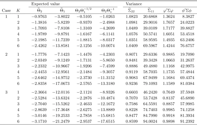
Remark 2. Theorem 1 indicates that each of the normalized statistics, when standardized by the appropriate moments, converges to a standard normal dis-tribution. Thus, to be able to make inference based on the normal distribution, we must first obtain the moments for each statistic. This can be done by Monte Carlo simulations. For this purpose, we make 10,000 draws of K+ 1 inde-pendent, scaled, random walks of lengthT = 1,000. By using these random walks as simulated Brownian motions, we construct approximations of the vector Brownian motion functionalsCi andCei. The means and the variances of these

simulated functionals are then used to approximate the asymptotic moments. The results obtained from this exercise are reported for up to six regressors in Table 1.

Remark 3. In view of Table 1, note that, although the distributions of the statistics are free of nuisance parameters, they do depend upon the deterministic specification of the test regression in (7), and on the number of regressors as reflected by dependence of Ui on Wid. Thus, the moments will also depend

on the deterministic specification and on the number of regressors. Moreover, notice that the distributions are independent of the short-run dynamics of the data generating process as captured by the first differences of the regressors. Thus, the statistics are asymptotically similar with respect to the short-run parameters in (7). In Table 1 we therefore only report simulated moments for the different deterministic cases and for different numbers of regressors. There is no need to tabulate separate moments for different lag orders.

Remark 4. As in the conventional unit root testing, the test regression in (7) involves estimating redundant trend parameters under the null. For example, in Case 2, the parameterδ1i vanishes under the restriction that αi = 0 but it

determines the mean of the error correction termyit−1−βi′xit−1when αi <0.

This redundancy turns up in the properties of the error corrections tests, which then depend on δ1i even under the null as seen by the dependence of Wid on

d. Under the alternative, the tests are consistent against cointegration with a constant but they are inconsistent against the more general alternative of cointegration with trend as equation (7) in Case 1 does not allow for a trend under the alternative. Thus, the tests permit for the constant term under the alternative by introducingδ1iin (7), which is irrelevant under the null.

Remark 5. So far, we have maintained Assumption 1 (c), which requires that xit is strictly exogenous. This is not necessary. In fact, as pointed out by

Banerjee et al. (1998), Assumption 1 (c) can be readily relaxed by making the error correction model in (4) conditional not only on the lags but also on the leads of the first difference of the regressors. The intuition is simple, and follows by the familiar dynamic least squares regression arguments of Saikkonen (1991). In particular, given that xit is weakly exogenous with respect to αi

and βi, eit must be uncorrelated with all current and past values of vit. But

this does not prevent eit from being correlated with the future values of vit,

which makes the new tests dependent on nuisance parameters reflecting this correlation. Therefore, in order to eliminate this dependency in case Assumption 1 (c) does not hold, we augment (4), and hence equations (6) through (8), not only with the lags but also with the leads ofvit. In what follows, to be able to

accommodate different lag and lead orders, we shall useqito denote the number

of leads for each cross-section.6

It is important that a statistical test is able to fully discriminate between the null and alternative hypotheses in large samples. The next theorem shows that the test statistics are consistent and that they are divergent under the alternative hypothesis.

Theorem 2. (Test consistency.) Under Assumption 1 and the alternative hypotheses H1g and H

p

1, then Gα, Gτ, Pα and Pτ diverges towards negative

infinity.

Remark 6. The proof of Theorem 2 is provided in the appendix. The theorem establishes that the divergence occurs towards negative infinity, suggesting that the tests can be constructed as one-sided using only the left tail of the normal distribution to reject the null hypothesis. Therefore, to test the null hypothesis of no cointegration based on the moments from Table 1, one simply computes the value of the standardized test statistic so that it is in the form specified

6

In contrast to the new tests, thet-ratio and coefficient type statistics of Pedroni (2004) do not require any correction to account for the absence of strict exogeneity, at least not asymptotically. Thus, in this respect, the residual-based approach is computationally more convenient. As we will show later in Section 6, however, the price in terms of small-sample performance of this greater convenience can be quite large.

in Theorem 1. This value is then compared with the left tail of the normal distribution. Large negative values imply that the null hypothesis should be rejected.

Remark 7. The proof of Theorem 2 uses the sequential limit theory. Although this allows for a relatively straightforward and tractable analysis, it cannot be used to obtain the joint rate of divergence under the two alternativesH₁gandH₁p, which is indicative of the relative power properties of the tests. It is, however, possible to establish the order of the statistics asT → ∞for a fixedN. In this case, it is shown in the appendix thatGα and Pα areOp(T) while Gτ andPτ

are Op(

√

T), which is in agreement with the results obtained by Phillips and Ouliaris (1990) for their residual-based time series tests. Given their faster rate of divergence, it is likely that the coefficient testsGαandPαhave higher power

thanGτ andPτ in samples whereT is substantially larger thanN.

5

Cross-sectional dependence

In this section, the results of the previous sections are generalized to account for dependence between the cross-sectional units.

As pointed out in Section 2, the our error correction tests are based on the assumption of independence, or at least zero correlation, over the cross-sectional units. Although the potential effects of the breakdown of this assumption is by now well understood, the allowance of such dependence has yet to become standard in the panel cointegration literature.

One solution would be to use data that has been demeaned with respect to common time effects. Thus, in this case, the statistics are calculated as before but with xeit = xit− _N1 PN_i=1xit in place of xit and eyit = yit− _N1 PN_i=1yit

in place ofyit, which does not alter their asymptotic distributions. However,

as demonstrated by Westerlund (2005b), although very convenient, subtracting the cross-sectional average in this way may not work very well, and may in fact result in a deterioration of the small-sample performance of the test.7 _Another disadvantage of this approach is that it do not permit for correlations that differ between pairs of individual time series, which seem like a more realistic assumption in many empirical applications.

One possible response to this is to employ the bootstrap approach, which makes inference possible even under very general forms of cross-sectional depen-dence. The particular bootstrap opted for in this section resembles that used by Chang (2004) and proceeds as follows.

7_{Unreported simulation results suggest that, although the cross-sectional demeaning is able}

to mitigate some effects of the dependence, the sizes of these tests can be very unreliable with massive distortions in many cases.

The first step is to fit the following least squares regression ∆yit = pi X j=1 b αij∆yit−j+ pi X j=0 b γij∆xit−j+beit. (9)

By using the residuals from this regression we then form the vector wbt =

(e_b′

t,∆x′t)′, where bet = (be1t, ...,ebN t)′ and ∆xt = (∆x′1t, ...,∆x′N t)′. It is this

vector that forms the basis for our bootstrap tests, and it is important that it is obtained from equation (9) with the null hypothesis imposed. Otherwise, if the null hypothesis is not imposed, this will render the subsequent bootstrap tests inconsistent. Note that, in Case 3, then (9) should be augmented with a constant to account for the trend inyit.

We then generate bootstrap samples w∗

t = (e∗′t,∆x∗′t)′ by sampling with

replacement the centered residual vector

e wt = wbt− 1 T₋1 T X j=1 b wj.

Note that by resamplingwetrather thanweit, we can preserve not only the

cross-sectional correlation structure ofeit but also any endogenous effects that may

run across the individual regressions of the system. The next step is to generate the bootstrap sample ∆y∗

it. This is accomplished

by first constructing the bootstrap version of the composite erroruitas

u∗ it = pi X j=0 b γij∆x∗it−j+e∗it,

where the least squares estimatebγijis obtained from the regression in (9). Given

pi initial values, we then generate ∆y∗itrecursively fromu∗it as

∆y∗ it = pi X j=1 b αij∆y∗it−j+u∗it, (10)

whereαbij is again obtained from (9). For initial values, we may use the firstpi

observations of ∆yit. However, as pointed out by Chang (2004), this does not

ensure the stationarity of ∆y∗

it. As an alternative approach, we may generate a

larger number,T+nsay, of ∆y∗

itand then discard the first nvalues. Because

this makes the initiation unimportant, we may simply use zeros to start up the recursion.

Finally, we generatey∗

itandx∗itwith the null hypothesis imposed. This is to

ensure the spuriousness of the generated sample as claimed under the null, and to make the resulting bootstrap tests valid. Thus, we obtainy∗

it andx∗it as y∗ it = yi∗0+ t X j=1 ∆y∗ ij and x∗it = x∗i0+ t X j=1 ∆x∗ ij,

which again requites initiation throughx∗

i0 andy∗i0. The value zero will do. Having obtained the bootstrap sampley∗

itandx∗it, we then obtain the

boot-strapped error correction statistic of interest, which is constructed exactly as its sample counterpart but withy∗

it andx∗itin place ofyit andxit. Denote this

initial bootstrap statistic by t∗

1. If we repeat this procedure S times, say, we obtaint∗

j for j = 1, ..., S, which is the bootstrap distribution of the statistic.

For a one-sided 5% nominal level test, we then obtain the lower 5% quantilet∗

C,

say, of the bootstrap distribution. The null hypothesis is rejected if the calcu-lated sample value of the statistic is smaller than t∗

C. Also, note that in case

the regressors are assumed to be weakly but not necessarily strictly exogenous, then the above bootstrap algorithm has to be modified to account for the leads of ∆xit.

6

Monte Carlo simulations

In this section, we study the small-sample properties of the new tests relative to those of some of the popular residual-based tests recently proposed by Pedroni (2004). For this purpose, a large number of experiments were performed using the following process to generate the data

∆yit = α(yit−1−βixit−1) + p X j=−q γ∆xit−j+eit, (11) ∆xit = vit. (12)

For simplicity, we assume that there is a single regressor, and that there is a common error correction parameterα. Hence,α= 0 under the null hypothesis, while α < 0 under the alternative. The results are organized in two parts depending on whether there is any cross-section dependence present or not.

In the first part with no cross-section dependence, we have three scenarios, which are all based on the following moving average process

eit = uit+φuit−1.

The innovationsuitandvitare both assumed to be normal variables with zero

mean and, unless otherwise stated, unit variance. The first two scenarios that we consider are concerned with the size of the tests, while the third is concerned with the power. The first scenario resembles the data generating process used by Pedroni (2004), and is designed to study the effects of serial correlation. In this case,γ = 0 andφ6= 0. By contrast, in the second scenario,φ= 0 andγ 6= 0. This scenario is taken from Westerlund (2005c), and the purpose is to evaluate the performance of the tests when the regressor is not strictly exogenous. For simplicity,pandq, the true number of lags and leads, are both set to one.

Finally, in the third scenario, we investigate the relative power of the tests, in which caseφ,pandqare all set to zero, so there is no serial correlation and only

the contemporaneous value of ∆xitenters (11). In particular, by settingγ= 1,

we can useβi to determine whether the common factor restriction is satisfied

or not. If the restriction is satisfied, thenβi = 1, whereas if it is not satisfied,

βi ∼ N(0,1). The degree of the violation is controlled by the signal-to-noise

ratio var(vit)/var(uit), which reduces to var(vit) if we assume that var(vit) = 1.

The second part of this section is designed to study the effects of cross-sectional dependence, and is parameterized as follows

eit = b(λi∆ft) +uit,

wherebis a scale parameter,λi is a loading parameter,ft∼N(0,1) anduit∼

N(0,1). Thus, in this setup,ftis a common factor that generates dependence

among the cross-sectional units. It enters (11) in first differences, which ensures that the common factor to yit is stationary. For simplicity, we set γ to zero,

so the regressor is strictly exogenous. All experiments are based on generating 2,000 panels withN individual andT+ 50 time series observations, where the first 50 observations for each series is discarded to attenuate the effect of the initial conditions, which are all set to zero.

For comparison, four of the residual-based tests of Pedroni (2004) are also simulated. Two are based on the group mean principle and are denotedZetand

e

Zρ, while the corresponding panel statistics are denotedZtandZρ. As explained

earlier, the Pedroni (2004) tests are based on the test regression in (5) and are thus subject to the common factor critique. Analogous to the new tests,Zetand

Zt are constructed as t-ratios, while Zeρ and Zρ are coefficient statistics. All

four tests are semiparametric with respect to the heteroskedasticity and serial correlation properties of the data.

As recommended by Newey and West (1994), all tests are constructed with the bandwidth chosen according to the rule 4(T /100)2/9_{. For the number of lags} and leads, we used two different rules, one depends on the data while the other depends onT. Specifically, for former, we used the Akaike information criterion, while for the latter, we used 2(T /100)2/9_{, which gives an overall lag and lead} expansion of the usual Newey and West (1994) rate 4(T /100)2/9_{. Consistent} with the results of Ng and Perron (1995), the maximum number of lags and leads for the Akaike criterion is permitted to grow withT at the same rate. The bootstrap tests are implemented using 200 bootstrap replications.

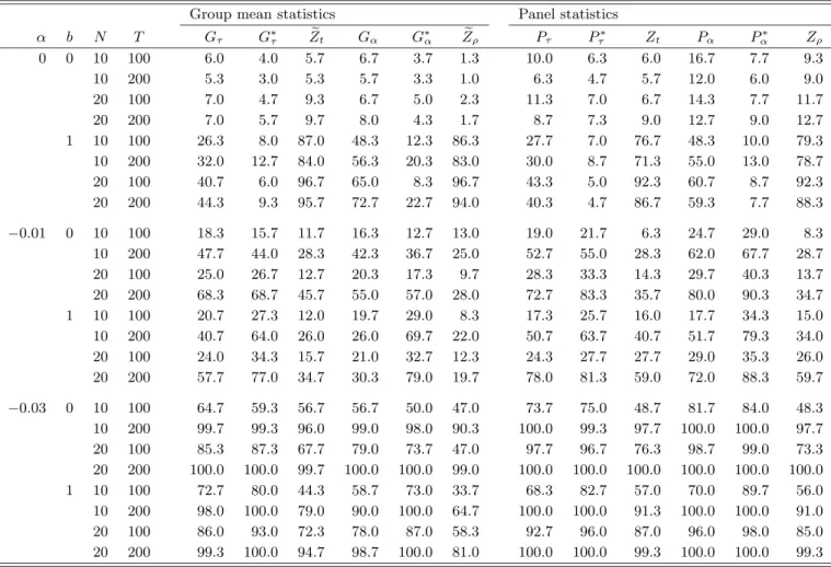
To keep the amount of table space manageable, we present only the size-adjusted power and the empirical size on the 5% level for Case 1 when there is no deterministic component. The results for the other cases were similar and did not change the conclusions. These are therefore omitted. Computational work was performed in GAUSS.

6.1

No cross-sectional dependence

In this case, there is no cross-sectional dependence, and we only consider the tests without the bootstrap proposal. Instead, we focus on the effects of serial

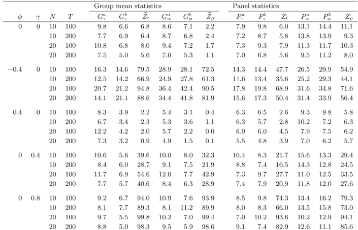
correlation and the absence of strict exogeneity, and on the common factor issue. Consider first the results on the size of the tests when α = 0, which are reported in Table 2. The data in the first scenario are generated with moving average errors, which makesφa convenient nuisance parameter to investigate. It has been well documented in simulation studies such as Haug (1996) that highly persistent moving average errors may cause substantial size distortions when testing the null of no cointegration in time series using residual-based tests with semiparametric type serial correlation corrections. Ng and Perron (1997) discuss the root of this problem to some length, and argue that it is the bias of the least squares estimate for the parameters of the spurious regression, and subsequently the autoregressive parameter of the errors, that causes these distortions. This bias is then imported into the semiparametric serial correlation correction, where it is further exacerbated by the difficulty inherent in long-run variance estimation.8

In agreement with these results, Table 2 show that the Pedroni (2004) tests tend to be severely oversized whenφis nonzero, especially when it is negative. In fact, with these tests, the results indicate that size can be up to 19 times the nominal 5% level. At the other end of the scale, we have the Gτ and Pτ

statistics, which have relatively small distortions. TheGαandPα statistics lie

somewhere in between. As expected, all tests perform well when φ = 0 and there is no persistence. We also see that there is not much difference between the error correction tests based on the two lag and lead rules, although the size is generally best for the tests based on choosing the number of lags and leads as a function ofT.

Given the findings of Ng and Perron (1997), a natural interpretation if these results is that the error correction test are less distorted because they do not rely on getting a good first-stage estimate of the level relationship. This lessens the bias induced not only in the estimation of the autoregressive parameter, but also in the semiparametric serial correlation correction. In other words, it seem likely that the error correction tests are less distorted because the bias in not compounded in the same way as for the residual-based tests.

The results from the second scenario are reported in the two bottom panels of Table 2. As expected, we see that the new tests are generally able to appro-priately correct for the fact that the regressor is no longer strictly exogenous. Among these tests, we see thatGτ andPτ generally perform best, which is in

agreement with the results from the first scenario. Of all the tests considered, the residual-based tests perform worst. In fact, based on the results reported in Table 2, rejection frequencies of up to 10 times the nominal 5% level are not uncommon, even whenγ= 0.4, so the strict exogeneity assumption is only moderately violated. Increasingγfrom 0.4 to 0.8 almost uniformly result in the

8_{Pedroni (2004) also discusses the difficulty in handling the effects of highly persistent}

moving average errors, and suggests modifying his tests along the lines of Ng and Perron (1997), which is expected to reduce the size distortions even in the panel context.

size of the residual-based tests going to 100%.

Although theoretically somewhat unexpected, these results are nevertheless consistent with the poor performance of the residual-based tests in the first scenario with serial correlation. Apparently, the problem with bias effects ex-tends also to the case with violations of strict exogeneity. In view of this, it seem desirable to employ some form of dynamic or fully modified least squares correction even for the residual-based tests.

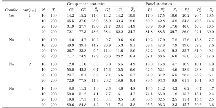
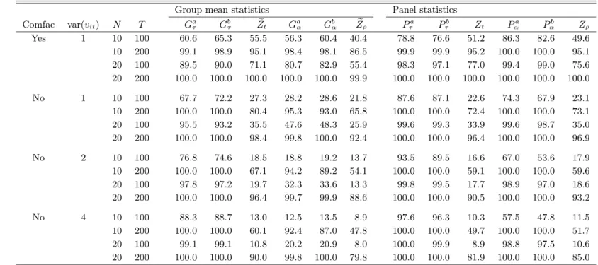
The power of the tests is evaluated next. Due to the different size properties of the tests, all powers are adjusted for size. Moreover, to be able to isolate the effects of the common factor restriction, bothγandφare set equal to zero. The results are reported in Table 3 for the case whenα=₋0.01, and in Table 4 for the case whenα=₋0.03.

It is seen that the new tests are almost uniformly more powerful than the residual-based tests by Pedroni (2004). In fact, the results suggest that the new tests are the most powerful even when the common factor restriction is satisfied, which is also what Banerjeeet al. (1998) find when simulating the time series versions of these tests. This is somewhat unexpected since the residual-based tests should be more efficient in this case. One possible explanation for this result is that the error correction tests are even more efficient, as they exploit the fact thatxitis weakly exogenous in this setup.

Although somewhat unexpected in the common factor case, the greater power of the error correction tests in the no common factor case is well in line with theory. In particular, in accordance with our discussion in Section 2, Tables 3 and 4 show that the relative power of the error correction tests in-creases monotonically as the signal-to-noise ratio inin-creases. This effect is further magnified by the fact that the power of the residual-based tests appears to be decreasing in var(vit), which is to be expected as large values of var(vit) will

tend to inflate the test regression in (5) with excess volatility.

The panel tests have the highest power, which is not surprising since they are based on the pooled least squares estimator of theα, and pooling is efficient under the homogenous alternative considered here. Among the panel tests, we see thatPαhas the highest power when the common factor restriction is

satis-fied, but thatPτbecomes more powerful as var(vit) increases and the restriction

is violated. Among the group mean tests, the results suggest thatGτ has the

highest power.

6.2

Cross-section dependence

In the cross-section dependent case, we use the scale parameterbto control the dependence. Ifb= 0, theneitreduces touitand there is no dependence, whereas

ifb = 1, then eit=λi∆ft+uit, which implies that E(eitejt) =λ2i ifi6=j so

the cross-sectional units are dependent. The results are reported in Table 5, where we use the star superscript to indicate the bootstrapped versions of the error correction statistics. Also, in this subsection, we drop the Akaike type

error correction tests and focus on the tests based setting the number of lags and leads as a function ofT, which greatly reduces the number of computations required.

Consider first the results on the size of the tests. As expected, we see that all tests perform well with only small distortions when b = 0 and there is no cross-sectional dependence. However, asb departs from zero, we see that there is a strong tendency for the asymptotic tests to overreject the null hypothesis. We also see that the magnitude of these distortions varies quite significantly. At one end of the scale, we have the Gτ and Pτ tests, which actually appear

to be quite robust to the cross-section correlation. At the other end, we have the residual-based tests, where the results suggest that the size can be very unreliable with severe distortions in most cases. As expected, the bootstrapped tests perform very well even under cross-sectional dependence.

Consider next the power of the tests. There are several things that are note-worthy. First, the power of the bootstrapped error correction tests is generally comparable with the power of their asymptotic counterparts. This result is very interesting because it suggests that we can correct the size of the tests with little or no cost in terms of power. Second, the residual-based tests are generally the least powerful, which corroborates the results reported in Tables 3 and 4.

6.3

Conclusions and their robustness

The simulation results presented in this section suggest that, under the main-tained assumption of weak exogeneity, the new tests perform well with good size and power in most panels. In particular, we find that the error correction tests have both better size accuracy and vastly superior power in comparison to the residual-based tests. We also find that the bootstrapped versions of the new tests are very effective in eliminating the effects of the cross-sectional dependence without sacrificing power.

These findings appear to be very robust, and extend to all sample sizes examined and to the cases with nonzero constant and trend terms. To also examine the effects of a violation of the weak exogeneity assumption, we carried out some simulations using the following process to generate the data

∆yit = (αy−γαx)(yit−1−βixit−1) +γ∆xit+eit,

∆xit = αx(yit−1−βixit−1) +vit.

Note that this is (11) and (12) withp and q set to zero,α = αy −γαx and,

perhaps most importantly, error correcting behavior for ∆xit. As before, we

assume thatβi ∼N(0,1) and γ= 1. We further disregard all effects of

cross-section dependence and serial correlation by making both eit and vit a draw

from the standard normal distribution.

Table 6 summarizes the results regarding the size and power of the tests at the 5% level with 10 cross-sectional units. In agreement with the discussion of

Section 2, we see that the error correction tests continues to perform well with good power whenαx is positive, but that the power falls significantly when it

is negative. In particular, we see that in the special case when bothαxandαx

are negative such thatαx< αx, then the error correction tests have no power

at all. The residual-based tests are also affected but not as dramatically as the error correction tests. Also, as expected, the size of the tests is not affected by the absence of weak exogeneity.

Thus, even though the error correction tests continues to perform well when αxis positive, in general we need the weak exogeneity assumption to ensure they

work properly. In spite of this, however, given their grater robustness in terms of both size accuracy and power, the overall impression of the Monte Carlo evidence presented is that the new tests compare favorably with the Pedroni (2004) tests. Also, in case weak exogeneity does not hold, it is probably better to analyze the data using the system-based approach of Larssonet al. (2001).9

7

Health care expenditures and GDP

In this section, we apply the new tests to data on health care expenditures (HCE) and GDP to demonstrate the use of these tests and to reassess previous empirical findings.

The relationship between HCE and GDP is the subject of a large portion of the literature in health economics. Many early contributions employed cross-sectional data to obtain estimates of this relationship. Without exception, it has been found that most of the observed variation in HCE can be explained by variation in GDP. However, many of these studies have been criticized for the smallness of their data sets and for the assumption that HCE is homoge-nously distributed across countries. More recent research has therefore resorted to panel data, which offers a number of advantages over pure cross-sectional data. For instance, using multiple years of data increases the sample size while simultaneously allowing researchers to control for a wide range of time invariant country characteristics through the inclusion of country specific constants and trends. In addition, with multiple time series observations for each country, researchers are able to exploit the presence of unit roots and cointegration in HCE and GDP.

9_{It should be noted, however, that there are simple ways to reduce the problem of}

endo-geneity, even for error correction based tests. For example, as pointed out by Zivot (2000), in situations withαi positive, a natural solution would be to simply perform a reverse test.

That is, the error correction tests are implemented in a conditional model forxitrather than

foryit. Zivot (2000) also presents several reasons for why weak exogeneity may not be too

much of a problem in practice. One reason is that it can be readily tested as a restriction on the unconditional model, which in the current panel data setting corresponds to the panel vector error correction model studied by Larssonet al. _{(2001). Another reason is that there}

appears to be strong support for the weak exogeneity assumption in many applications, see Zivot (2000) and the references therein.

This avenue is taken by Hansen and King (1996), who examine a panel spanning the years 1960 to 1987 across 20 OECD countries. They show that, if one examines the time series for each of the countries separately, one can only rarely reject the unit root hypothesis for either HCE or GDP. Moreover, their country specific tests rarely reject the hypothesis of no cointegration. McCoskey and Selden (1998) use the same data set as Hansen and King (1996). Based on the panel unit root proposed by Imet al. (2003), the authors are able to reject the presence of a unit root in both HCE and GDP. Once a linear time trend has been accommodated, however, the null hypothesis cannot be rejected.

Hansen and King (1998) question the preference of McCoskey and Selden (1998) for omitting the time trend from their main results, and argue that this may lead to misleading inference. Indeed, using a panel covering 24 OECD coun-tries between 1960 and 1991, Blomqvist and Carter (1997) challenge the findings of McCoskey and Selden (1998). Drawing on a battery of tests, including the panel unit root test of Levinet al. (2002), the authors conclude that HCE and GDP appear to be nonstationary and cointegrated. Gerdtham and L¨othgren (2000) present confirmatory evidence using a panel of 21 OECD countries be-tween 1960 and 1997. Similarly, using a panel of 10 OECD member countries over the period 1960 to 1993, Roberts (2000) found clear evidence suggesting that HCE and GDP are nonstationary variables. The results of cointegration were, however, not conclusive.

Apparently, although the evidence seems to support the unit root hypothesis for HCE and GDP, it is less conclusive on the cointegration hypothesis. One possible explanation for these differences may be the common factor restriction implicitly imposed when testing the null hypothesis of no cointegration using residual-based procedures as in Hansen and King (1996).10

In this section, we verify this conjuncture by using a panel consisting of 20 OECD countries and covering the period 1970 to 2001. For this purpose, data on annual frequency has been acquired through the OECD Health Data 2003 database. Both HCE and GDP are measured in per capita terms at constant 1995 prices and are transformed in logarithms. Moreover, since both variables are clearly trending, we follow the earlier literature and model HCE and GDP with a linear time trend in their levels. An obvious interpretation of such a trend is that it accounts, in part, for the impact of technological change.

The basic model we postulate between HCE and GDP, denotedHitandYit,

respectively, is the following simple log-linear relationship

ln(Hit) = µi+τit+βiln(Yit) +eit. (13)

The first step in our analysis of this relationship is to test whether the variables are nonstationary or not. To this effect, we employ a battery of unit root tests, which can be classified into two groups depending on whether they allow for

10_{Since the data sets used in the previous studies are nearly identical, any differences in}

cross-sectional correlation or not. The first group consists of theZttest of Im

et al. (2003) and the Harris and Tzavalis (1999)ϕblsdvtest, which are both based

on the assumption of no cross-sectional dependence.

However, like many other macroeconomic variables, HCE and GDP usually exhibit strong comovements across countries. The second group of tests allows for such cross-sectional dependence by assuming that the variables admit to a common factor representation. It includes theG++_ols,Pmand Z tests of Phillip

and Sul (2003), theta andtbtests of Moon and Perron (2004) and the Bai and

Ng (2004)Pc e test.

All tests are normally distributed under the common null hypothesis of non-stationarity, and all tests exceptϕ_blsdv, ta andtb permit the individual

autore-gressive roots to differ across the cross-sectional units. The direction of the divergence under the alternative hypothesis determines whether we should use the right or left tail of the normal distribution to reject the null. TheZt,ϕblsdv,

G++_ols, Pm, ta and tb statistics diverge to negative infinity and are compared to

the left tail, whereas theZandPc

e statistics diverge to positive infinity, and are

thus compared to the right tail.

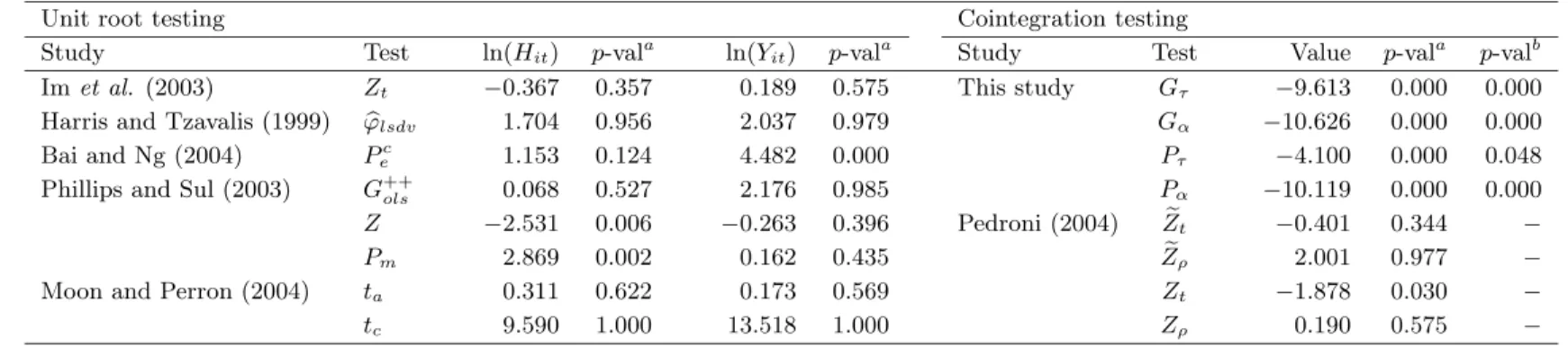
For the implementation of the tests, we use the Bartlett kernel, and all band-widths and lag lengths are chosen according to 4(T /100)2/9_{. The number of lags} and leads are chosen by the Akaike criterion. To determine the number of com-mon factors, we use the Bai and Ng (2004)IC1criterion with a maximum of five factors. The test results reported in Table 7 indicate that in only three out of the 16 cases do we end up with a rejection of the null at the 1% level of significance. We therefore conclude that the variables appear to be nonstationary.

The second step in our empirical analysis is to test whether HCE and GDP are cointegrated. One way to do this is to use the residual-based approach, and to subject the regression residuals from (13) to a unit root test. The results presented in Table 7 based on using this procedure suggest that we cannot reject the null hypothesis of no cointegration at the 1% level for any of the residual-based tests. In fact, even if we look at the most liberal 10% level, we end up rejecting the null for three out of the four tests. As pointed out earlier, however, the prospect of imposing an invalid common factor restriction may well result in this procedure having very low power in samples as small as ours. In that case, the error correction tests may be able to produce more powerful tests.

Our results confirm this conjuncture. In particular, unreported estimation results show that the standard errors of the individual test regressions for the residual-based tests are much larger in comparison to those of the corresponding error correction test regressions, which is indicative of an invalid common factor restriction. To tests whether this is in fact the case, we performed a series of individual Wald tests, which all resulted in a strong rejection of the common factor restriction.

The implication of these results is that the new tests may be more powerful. The calculated values of the error correction statistics are presented along with

both asymptotic and bootstrappedp-values in Table 7. When using the asymp-toticp-values, we see that all four tests lead to a clear rejection of the null, even at the most conservative 1% level, which we take as strong evidence in favor of cointegration. There is no difference depending on whetherαiis restricted to be

equal for allior not. Based on the bootstrappedp-values, we end up with one rejection, forPτ, at the 5% level. However, since this rejection is only marginal,

and since the homogenous alternative hypothesis considered for this particular test may be overly restrictive, we choose to interpret these results as evidence in favor of cointegration between HCE and GDP.

8

Conclusions

In this chapter, we propose four new panel cointegration tests that are designed to test the null hypothesis of no cointegration by testing whether the error correction term in a conditional error correction model is equal to zero. If the null hypothesis of no error correction is rejected, then the null hypothesis of no cointegration is also rejected. Each test is able to accommodate individual specific short-run dynamics, including serially correlated error terms and non-strictly exogenous exogenous regressors, individual specific intercept and trend terms, as well as individual specific slope parameters. A bootstrap procedure is also proposed to handle applications with cross-sectionally dependent data.

Using sequential limit arguments, we show that the new tests have limiting normal distributions, and that they are consistent. These results are verified in small samples using Monte Carlo simulations. In particular, given that the regressors are weakly exogenous with respect to the parameters of interest, we find that the new tests show both better size accuracy and higher power than the residual-based tests recently developed by Pedroni (2004). We further show that this difference in power arise mainly because the residual-based tests ignore potentially valuable information by imposing a possibly invalid common factor restriction. On the other hand, we also find that the power of the new tests can be quite adversely affected if weak exogeneity fails, in which case the system-based approach of Larssonet al. (2001) is recommended.

In our empirical application, we provide evidence suggesting that HCE and GDP are cointegrated once the difference between the short- and long-run rela-tionships has been accounted for.

Appendix: Mathematical proofs

This appendix proves the asymptotic results for the new test statistics. For convenience, we shall prove the results for Case 1 with no deterministic compo-nents. For brevity, the notations introduced in the main text are taken as given and are thus not repeated. Moreover, for any variablezit, we usezit∗ to indicate

the error from projecting zit onto onto xit−1, and (zit)p to indicate the error

from projecting zit onto wit = (∆yit−1, ...,∆yit−pi,∆x′it, ...,∆x′it₋pi)

′_{. Thus,} (zit)p=zit−w′itai, where ai is a vector of projection parameters.

Lemma A.1. (Preliminaries for Theorem 1.) Under Assumption 1 and the null hypothesis, asT _{→ ∞} (a) T−1/2_y it ⇒ 1 αi(1) (γi(1)′B2i+B1i); (b) T−2PT t=2(yit∗−1)2p ⇒ 1 αi(1)2 σi2 Z 1 0 Ui2; (c) T−1PT t=2(yit∗−1)p(e∗it)p ⇒ 1 αi(1) σ2i Z 1 0 UidVi.

Proof of Lemma A.1

Consider (a). The model (4) in Case 1 can be written as

αi(L)∆yit = αi(yit−1−β′ixit−1) +uit, (A1)

whereuit=γi(L)′vit+eit. By using the Beveridge-Nelson (BN) decomposition

ofγi(L) as γi(L) =γi(1) +γi∗(L)(1−L), we obtain uit = γi(L)′vit+eit = γi(1)′vit+γi∗(L)′∆vit+eit. Therefore, asT _{→ ∞}we get T−1/2 t X j=2 uij = γi(1)′T−1/2 t X j=2 vij+γi∗(L)′T−1/2vit+T−1/2 t X j=2 eij = γi(1)′T−1/2 t X j=2 vij+T−1/2 t X j=2 eij+op(1) ⇒ γi(1)′B2i+B1i. (A2)

Next, we use the BN decompositionαi(L) =αi(1) +α∗i(L)(1−L) ofαi(L),

which implies that

which, under the null, can be rewritten as ∆yit = −α ∗ i(L) αi(1)∆ 2_y it+ 1 αi(1)uit.

This implies (a) as can be seen by writing T−1/2 t X j=2 ∆yij = −α ∗ i(L) αi(1) T−1/2_∆y it+ 1 αi(1) T−1/2 t X j=2 uij = 1 αi(1)T −1/2 t X j=2 uij+op(1) ⇒ _α1 i(1) (γi(1)′B2i+B1i),

where the last result follows from (A2).

Next, consider (b). By using the rules for projections, the sumPT_t=2(y∗

it−1)2p can be written as T X t=2 (y∗ it−1)2p = T X t=2 y∗2 it−1− T X t=2 y∗ it−1w∗′it à _T X t=2 w∗ itw∗′it !−1 _T X t=2 w∗ ityit∗−1, (A3) where T X t=2 y∗ it−1wit∗′ = T X t=2 yit−1w′it− T X t=2 yit−1x′it−1 · à _T X t=2 xit−1x′it−1 !−1 _T X t=2 xit−1w′it. (A4)

By Lemma 2.1 of Park and Phillips (1989), we have thatPT_t=2yit−1w′it=Op(T),

PT

t=2yit−1x′it−1 = Op(T2), PTt=2xit−1x′it−1 = Op(T2) and PTt=2xit−1w′it =

Op(T). Therefore,PT_t=2yit∗−1w∗′it=Op(T).

Similarly, PT_t=2w∗

itw∗′it in (A3) may be expanded as T X t=2 w∗ itwit∗′ = T X t=2 witwit′ − T X t=2 witx′it−1 Ã _T X t=2 xit−1x′it−1 !−1 _T X t=2 xit−1wit′ = Op(T) +Op(T)Op(T−2)Op(T) = Op(T). (A5)

Thus, by using (A3) to (A5), we can show that

T X t=2 (y∗ it−1)2p = T X t=2 y∗2 it−1+Op(T)Op(T−1)Op(T)

= T X t=2 y∗2 it−1+Op(T), (A6)

For the remaining term in (A6) we use (a), which implies T−1/2_y∗ it−1 = T−1/2yit−1−T−2 T X t=2 yit−1x′it−1 · Ã T−2 T X t=2 xit−1x′it−1 !−1 T−1/2_x it−1 ⇒ _α1 i(1) (γi(1)′B2i+B1i)− 1 αi(1) Z 1 0 (γi(1)′B2i+B1i)B2′i · µZ 1 0 B2iB2′i ¶−1 B2i,

where the last expression can be manipulated to obtain 1 αi(1) B1i− 1 αi(1) Z 1 0 B1iB2′i µZ 1 0 B2iB2′i ¶−1 B2i = 1 αi(1)σiVi− 1 αi(1)σi Z 1 0 ViWi′ µZ 1 0 WiWi′ ¶−1 Wi = 1 αi(1) σiUi.

Putting everything together, we get T−2 T X t=2 (y∗ it−1)2p = T−2 T X t=2 y∗2 it−1+op(1) ⇒ 1 αi(1)2 σi2 Z 1 0 Ui2, which establishes (b).

Finally, consider (c). We have

T X t=2 (y∗ it−1)p(e∗it)p = T X t=2 y∗ it−1e∗it− T X t=2 y∗ it−1wit∗′ · Ã_XT t=2 w∗ itwit∗′ !−1 _T X t=2 w∗ ite∗it. (A7)

By using the same arguments as before, it is clear that

T X t=2 w∗ ite∗it = T X t=2 witeit− T X t=2 witx′it−1 Ã _T X t=2 xit−1x′it−1 !−1 _T X t=2 xit−1eit = Op( √ T) +Op(T)Op(T−2)Op(T)

= Op(

√

T),

which, together with (A4), (A5) and (A7), implies that

T X t=2 (y∗ it−1)p(e∗it)p = T X t=2 y∗ it−1e∗it+Op(T)Op(T−1)Op( √ T) = T X t=2 y∗ it−1e∗it+Op( √ T). By using (a), the limit of the remaining term becomes

T−1 T X t=2 y∗ it−1e∗it = T−1 T X t=2 yit−1eit−T−2 T X t=2 yit−1x′it−1 · Ã T−2 T X t=2 xit−1x′it−1 !−1 T−1 T X t=2 xit−1eit ⇒ _α1 i(1) Z 1 0 (γi(1)′B2i+B1i)dB1i − _α1 i(1) Z 1 0 (γi(1)′B2i+B1i)B2′i µZ 1 0 B2iB2′i ¶−1 · Z 1 0 B2idB1i,

where the last expression is 1 αi(1) Z 1 0 B1idB1i− 1 αi(1) Z 1 0 B1iB′2i µZ 1 0 B2iB′2i ¶−1Z ₁ 0 B2idB1i = 1 αi(1) σ2i Z 1 0 VidVi − _α1 i(1)σ 2 i Z 1 0 ViWi′ µZ 1 0 WiWi′ ¶−1Z ₁ 0 WidVi = 1 αi(1) σ2i Z 1 0 UidVi. This proves (c). ¥ Proof of Theorem 1

Consider first the group mean statistics. Note thatαbi may be written as

b αi = Ã _T X t=2 (y∗ it−1)p !−1 _T X t=2 (y∗ it−1)p(∆y∗it)p. (A8)