Quantitative Modeling of Integrase Dynamics Using a Novel Python Toolbox for Parameter Inference in Synthetic Biology

(1)

Quantitative Modeling of Integrase Dynamics Using a Novel

Python Toolbox for Parameter Inference in Synthetic Biology

Anandh Swaminathan

1,∗

, Victoria Hsiao

2

, Richard M. Murray

1,3

March 27, 2017

1. Computing & Mathematical Sciences, California Institute of Technology, Pasadena, CA. 2. Amyris, Emeryville, CA.

3. Biology and Biological Engineering, California Institute of Technology, Pasadena, CA. * Corresponding Author: Anandh Swaminathan, aswamina at caltech dot edu.

Subject categories: synthetic biology, systems biology, Python, stochastic simulation, stochastic chemical reactions, cell lineage simulations, integrase circuits, cell free systems, serine integrases Keywords: Single cell simulations / Python for synthetic biology / Fast simulation of stochastic chemical

reactions / integrase circuits / serine integrases / cell free systems Running Title: Python package for simulation of biocircuits

(2)

Abstract

The recent abundance of high-throughput data for biological circuits enables data-driven quanti-tative modeling and parameter estimation. Common modeling issues include long computational times during parameter estimation, and the need for many iterations of this cycle to match data. Here, we present BioSCRAPE (Bio-circuit Stochastic Single-cell Reaction Analysis and Parameter Estimation) - a Python package for fast and flexible modeling and simulation for biological circuits. The BioSCRAPE package can be used for deterministic or stochastic simulations and can incor-porate delayed reactions, cell growth, and cell division. Simulation run times obtained with the package are comparable to those obtained using C code - this is particularly advantageous for computationally expensive applications such as Bayesian inference or simulation of cell lineages. We first show the package’s simulation capabilities on a variety of example simulations of stochas-tic gene expression. We then further demonstrate the package by using it to do parameter inference for a model of integrase dynamics using experimental data. The BioSCRAPE package is publicly available online along with more detailed documentation and examples.

(3)

Introduction

Quantitative approaches to both synthetic and systems biology rely on modeling and simulation of biological circuits. Biological circuits are systems where different components, typically genes, can interact with each other via different types of molecular interactions including transcriptional activation and repression and sequestration. These interactions are typically modeled as a system of chemical reactions where each reaction has a certain reaction rate. The rate can be modeled using mass action kinetics (Del Vecchio and Murray, 2014), but many reactions in biological circuits have sigmoidal saturating reaction rates. These reactions are typically modeled using Hill functions (Del Vecchio and Murray, 2014) .

Given the reaction model for a biological circuit, there are many different ways to simulate the model. First of all, regardless of simulation framework, it is necessary to specify the values of the parameters in the model along with the initial levels of the model species. By treating the reaction rates as deterministic bulk rates and using ordinary differential equations (ODE’s), one might perform a deterministic simulation of the system.

On the other hand, it also common to treat the reaction rates as propensities for discrete reactions to fire and to model the system as a set of stochastic chemical reactions (Gillespie, 1977). Biological circuits can often be noisy (Elowitzet al, 2002; Eldar and Elowitz, 2010) especially at low molecular copy numbers, and a stochastic model is often necessary to capture the noise characteristics of a circuit.

Some other common features in biological circuit models are delay and cell growth and division. Pro-cesses like protein production are not instantaneous, and there is often a significant delay between when transcription of a gene is initiated and when a mature protein is produced. This type of delay can lead to nontrivial behavior such as oscillations (Strickeret al, 2008), and thus it is often important to incorporate delay into the modeling framework. Additionally, delays can be both fixed and distributed in their duration. While adding a fixed delay to a biological circuit might destabilize the circuit and create oscillatory behavior, distributing that delay across multiple durations might maintain circuit stability (Gomezet al, 2016).

Cell growth and division are also critical aspects of biological circuits that operate in single cells. Typ-ically, a dilution term in the model accounts for cell growth. However, in stochastic models, modeling the continuous dilution process with a stochastic and discrete degradation reaction might not be accurate. Another source of noise is the partitioning of molecules between daughter cells at cell division (Huh and Paulsson, 2011). In fact, it can be difficult to distinguish between noise in gene expression and noise from molecular partitioning (Huh and Paulsson, 2011). Therefore, modeling cell growth as well as division and partitioning is important for investigating noise in gene expression across a lineage of cells.

In order to validate these types of models of biological circuits against actual data, it is often helpful to have a large amount of experimental data measured for the circuit. For deterministic models, it is of-ten helpful to have data collected at many different operating conditions, while for stochastic models, it is also helpful to have large sample sizes. The increasing use of technologies for lab automation as well as high throughput measurement techniques involving liquid handling (Mooreet al, 2016) and flow cytometry (Sachset al, 2005; Zechneret al, 2012) makes this data collection more easy to do.

Using experimental data, one can fit parameters for models of biological circuits and tune the models to better match qualitative trends in the data. In this workflow, it is often necessary to add or remove reactions from the model or to perform a different type of simulation. For example, one might decide that a circuit behaves too noisily for deterministic simulations and want to switch to a stochastic simulation framework. If delays are playing a significant role in the dynamics, one might want to incorporate previously unmodelled delays into the model.

The most attractive methods for performing parameter inference on these models are those that use Bayesian inference (Golightly and Wilkinson, 2011; Komorowskiet al, 2009), because these methods pro-vide a full posterior distribution over the parameter space. This gives insight into the accuracy and iden-tifiability of the model. Also, such an approach allows for an easy comparison between different model classes using the model evidence. The drawback of these approaches is that their implementation is com-putationally expensive and is based on repeated forward simulations of the model within the framework of Markov chain Monte Carlo (MCMC) (Golightly and Wilkinson, 2011). Therefore, it is important to have the underlying simulations running as fast as possible in order to speed up computation time.

This paper presents BioSCRAPE (Bio-circuit Stochastic Single-cell Reaction Analysis and Parameter Estimation), which is a Python package for fast and flexible modeling and simulation of biological circuits.

(4)

The BioSCRAPE package uses Cython (Behnelet al, 2011), an extension for Python that compiles code using a C compiler to vastly increase speed. This helps assuage the computational time issues that arise in parameter estimation. Additionally, the paper provides a flexible text based framework for specifying models of biological circuits as well as a set of simulators that can perform deterministic and stochastic simulations as well as incorporate delay and cell growth and division. If a researcher needs to change a circuit model, he or she can simply edit a few lines in a text file to make the change. If a researcher needs to simulate a circuit differently, he or she can simply select a different simulator to use.

Some popular software packages that do somewhat similar tasks to the BioSCRAPE package are MAT-LAB’s SimBiology toolbox (MATLAB, 2016) and Stochpy (Maarleveldet al, 2013). However, the BioSCRAPE package runs simulations faster than either and also supports simulations of whole cell lineages as well as more general reaction rates.

The following sections contain an overview of the model specification language as well as some exam-ples of simulations performed using the package. Additionally, the penultimate section contains a demon-stration of BioSCRAPE to perform parameter estimation for integrase DNA recombination dynamics based on experimental data. More detailed documentation and the code for the examples as well the package itself are available online.1

A flexible modeling language for biological circuits

The first piece of the software package is a flexible text based modeling framework. The framework uses XML to specify the reactions that make up the interactions of a model. Once the XML file for a model is loaded into the software package, it can then be simulated using whatever method is desired.

Another common XML based specification language for biological models is the Systems Biology Markup Language (SBML) (Huckaet al, 2003). The SBML language is very general and can describe a wide vari-ety of biological systems, but it is also complex. Therefore, the BioSCRAPE package instead uses a very simple modeling language that only specifies model reactions.

The XML language consists of a simple specification of reactions along with propensities and delays. Code Block 1: Simple examples of XML reactions

</reaction>

</reaction>

Code block 1 contains an example specifying two reactions. The first reaction is a transcription reaction with delay. ThereactionXML tag contains atextfield and anafterfield, where thetextfield contains the part of the reaction that happens initially and theafterfield contains the part of the reaction that occurs after a delay. The products and reactants are separated from each other by the--characters, and multiple products and reactants can be included by separating them with plus signs.

The first reaction above is a delayed transcription reaction, as the only thing that happens in this reaction is that mRNA appears after a delay. The second reaction is a degradation reaction without delay as the only thing that happens is that mRNA disappears.

Thepropensityfield specifies the reaction rate. In this case, both reactions have mass action propen-sities. For mass action propensities, the rate parameter is given by the attributekand thespeciesattribute specifies the species involved. In this case, mRNA is produced with a constitutive propensity ofbeta, so there are no species involved, and the rate is specified to be the parameterbeta. For the second reaction,

(5)

the degradation rate of mRNA is given bydelta_m×mRNA. If more than a single species is involved in a mass action reaction rate, the species can separated by*signs.

Finally, a delay must also be specified for each reaction. If there is no delay, the delay type can be set tononeas in the second reaction. However, if there is a delay, the type of delay must be specified along with any associated parameters. The transcription reaction above has a fixed delay, and thus a parameter is required to specify the duration of the fixed delay. If the delay is distributed with a gamma distribution, then the shape and scale of the distribution must be specified.

Code Block 2 shows the initialization process for parameter values and initial species levels. Both the initial conditions and the parameter values can be modified from a Python script after the model has been loaded as well, so it is not necessary to edit the XML file and load the model every time a parameter or initial condition is changed.

Code Block 2: Initialization of parameters and species <parameter name="beta" value="2.0" />

The reactions in Code block 1 and the parameters and initial species values in Code block 2 are both part of an XML file describing a simple model of gene expression with delayed transcription and translation and the usual linear degradation of mRNA and protein. This model will be simulated in many different ways in the next section, and its full XML can be found in Appendix 1.

Flexible simulation of biological circuits

This section demonstrates the different types of simulations that can be performed with the BioSCRAPE package using the model of delayed gene expression from Appendix 1 as an example.

The package is capable of performing stochastic simulations with and without delay and with and without cell growth and division. However, deterministic simulations only work without delays or cell division.

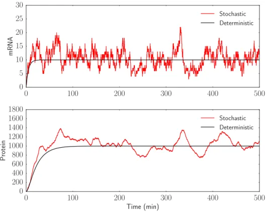
As a first pass, the simple gene expression model can be simulated both deterministically and stochas-tically ignoring delays and cell division. Importantly, switching between a deterministic and stochastic simu-lation only requires a single line to be modified in the code. The simusimu-lation output is the mRNA and protein trajectories over time.

Figure 1 shows the simulated deterministic and stochastic trajectories. As expected, the deterministic simulation smoothly goes to a steady state of 10 mRNA molecules and 1000 proteins, while the stochastic simulation bounces around the deterministic value. Because the mRNA production and degradation events in this model represent a standard birth death process, it can be analytically determined that the steady state distribution of mRNA should be a Poisson distribution with parameterλ= 10, and that the autocorrelation time for the mRNA trajectory should be exp(0.2t). Both of these analytical solutions can be compared to the empirical probability distribution and autocorrelation for mRNA. These can be computed using a longer simulation of 50,000 simulation minutes. The results are presented in Figure 2.

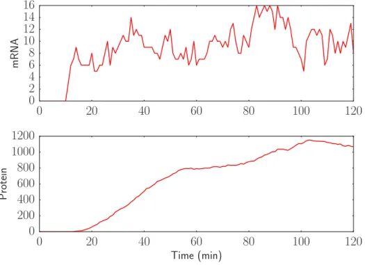
The next step is to incorporate the delays specified in the model. The transcriptional delay in the model is a fixed delay of 10 minutes, while the translational delay is gamma distributed with a mean of 10 minutes. Again, switching from a simulation without delay to one that incorporates delay only requires changing a few lines of code. Only a single line of code is required to change the simulator, but as the initial conditions for a delayed simulation include a history of queued reactions, this initial condition must be constructed as well. The results from a delayed simulation of the model are presented in Figure 3. As expected, the mRNA

(6)

0

100

200

300

400

500

0

5

10

15

20

25

30

mRNA Stochastic Deterministic

0

100

200

300

400

500

Time (min)

0

200

400

600

800

1000

1200

1400

1600

1800

Protein Stochastic Deterministic

Figure 1: Deterministic and stochastic simulations of simple gene expression without delay

0 5 10 15 20 25 30 mRNA Count 0.00 0.02 0.04 0.06 0.08 0.10 0.12 0.14 Probabilit y Mass Empirical Exact 0 5 10 15 20 25 Lag time 0.0 0.2 0.4 0.6 0.8 1.0 Auto co rrelation fo r mRNA Simulations Exact

Figure 2: Empirical steady state mRNA distribution and autocorrelation times match the analytical answers.

turns on at 10 minutes, and the protein turns on at around 20 minutes. Because the delay is distributed, the protein actually starts increasing slightly before 20 minutes have elapsed.

Cell growth and division can also be incorporated into the simulation. The dynamics of cell growth and division are not specified in the model XML file, so they must be specified in the Python simulation script. The model must specify the rate of cell growth as well as the time and volume at which the cell divides. The model of cell growth and division used in the package consists of deterministic exponential growth and cell division upon reaching a certain volume threshold. A noise parameter allows for incorporating some stochasticity into the dynamics. The daughter cells in this model are also exactly half the size of the mother cell.

(7)

0

20

40

60

80

100

120

0

2

4

6

8

10

12

14

16

mRNA

0

20

40

60

80

100

120

Time (min)

0

200

400

600

800

1000

1200

Protein

Figure 3: Delayed simulation shows abrupt delay in mRNA production and smooth delay in protein produc-tion.

The method for partitioning molecules between daughter cells must also be specified in the simulation Python script. Currently, the model for molecular partitioning is one in which the molecules are partitioned binomially between the two daughter cells in a manner that is consistent with the daughter cell volumes. For example, if one daughter cell is twice as big as the other, then it receives about two thirds of the molecules. The reaction rates in the model also become volume dependent when performing a volume based simulation. For example, a unimolecular reaction does not depend on volume, but a bimolecular mass action reaction rate will scale asVolume−1because the odds of two molecules finding each other decrease as the volume increases. Similarly, in Hill function rates, the transcription factor in the Hill function is replaced by its concentration when doing volume based simulations, since the concentration sets the equilibrium binding of the transcription factor to the DNA. These changes happen automatically when switching to a volume based simulation.

The output of a lineage simulation is a set of cell traces, where each trace contains a cell’s volume and species trajectories over a single cell cycle. Each cell trace also may or may not have a parent cell trace as well as daughter cell traces. This data structure is similar to the one used in the Schnitzcells microscopy image analysis software (Younget al, 2012).

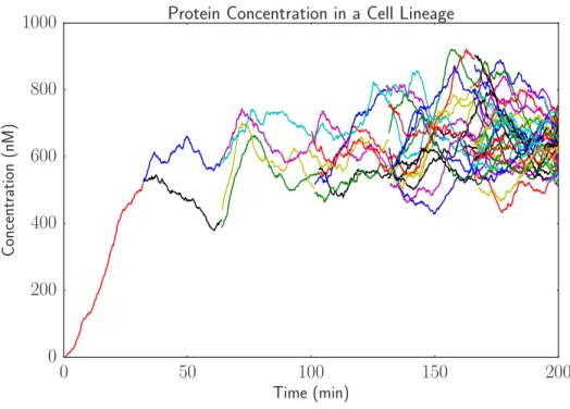
A simulation of the simple gene expression model ignoring delays is provided in Figure 4 for a lineage of cells with a division time of 33 minutes. In this figure, the plotted quantity is protein concentration, which is molecules of protein per cell divided by the current cell volume. Here, the cell volume ranges between 1.0 and 2.0, and the volume unit can be thought of as a characteristic E. coli cell volume. A common assumption inE. coli models is that 1 molecule per cell corresponds to a concentration of 1 nM, and so 1 molecule per characteristic cell volume here is assumed to be 1 nM.

The initial single cell trajectory branches into more and more trajectories as the cell divides. At cell division, the concentration of protein in each daughter cell can change discontinuously. This occurs because of the noise in molecular partitioning. Because the proteins are high copy number, this noise is fairly small in this example.

(8)

0

50

100

150

200

Time (min)

0

200

400

600

800

1000

Concentration (nM)

Protein Concentration in a Cell Lineage

Figure 4: Simulation with cell growth and partitioning shows variation in gene expression across a lineage of cells.

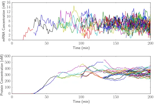
incorporates both cell lineages and delays. The simple gene expression model with delays can be simulated using the same model of cell growth and division (33 minute division time) as the one used to produce Figure 4. In this case, the transcription and translation delay are set to 16.5 minutes each, for a total delay in protein production of one 33 minute cell cycle. The results are shown in Figure 5.

While the results from Figure 5 look qualitatively similar to the results in Figure 4, it is important to note that the final level of steady state protein expression in the simulation with delay is only about 300 proteins versus the 600 protein steady state in the simulation without delay. The reason for this is that because of the delay, the amount of protein that is being produced at a given time is proportional to the number of cells that existed 33 minutes ago. Because the delay is one cell cycle, the amount of protein production is effectively half of what it would be without delay. This is consistent with the steady state protein expression with delay being about half as much as without delay.

This result provides insight for selection of fluorescent proteins for use in exponentially growing colonies of cells. It might be better to use fast maturing fluorescent proteins that are dimmer on average compared to bright fluorescent proteins that mature slowly, because the signal loss due to the long delay might outweigh the additional brightness per molecule. For example, a fluorescent protein that takes an extra cell cycle time to mature must be twice as bright in order to generate the same fluorescent signal at steady state.

Fast simulation of biological circuits

In addition to the framework for flexible modeling and simulation of biological circuits described in the pre-vious sections, the third critical aspect of a software package for quantitative analysis of biological circuits is speed. This package is written using Cython (Behnelet al, 2011), a language extension for Python that creates compiled Python libraries. Some alternative methods for doing stochastic simulation are to use the SimBiology toolbox in MATLAB (MATLAB, 2016), write code in C from scratch, or to use a pure Python library such as StochPy (Maarleveldet al, 2013). In this section, the simulation speed of the BioSCRAPE package is benchmarked against these other three common simulation options.

(9)

0 50 100 150 200 Time (min) 0 2 4 6 8 10 12 14 16 mRNA Concentration (nM) 0 50 100 150 200 Time (min) 0 100 200 300 400 500 600 Protein Concentration (nM)

Figure 5: Simulation with cell growth and partitioning in addition to delay shows reduced steady state gene expression across a lineage of cells.

The benchmark test used for comparing the speed of these different simulators is to simulate the simple gene expression model from the previous sections with code available in Appendix 1. As MATLAB SimBi-ology does not support delayed reactions, the system was simulated ignoring delays for 100,000 minutes starting from an initial condition of zero. Additionally, both SimBiology and StochPy output each step of the stochastic simulation as opposed to outputting the system state at specific times. For the simulation conditions in this system, the number of steps taken in 100,000 minutes is always around ten million steps. Therefore, to make the comparison fair, the simulation in the BioSCRAPE package is done with ten million desired time points in order to keep the output size the same in all cases. Finally, the C code is a pure C im-plementation of the simulation using the same fixed interval algorithm as the BioSCRAPE Python package, so the C implementation is also run with ten million desired time points.

Table 1: A speed comparison between this Python package and other common simulation platforms.

Software Benchmark time (s) Speed-up

SimBiology 5.8 8.3x

StochPy 190 270x

C 0.38 0.54x

BioSCRAPE package 0.70

-The simulation times are available in Table 1. -The table shows that the BioSCRAPE package outper-forms SimBiology by almost one order of magnitude, but it outperoutper-forms the pure Python StochPy package by a factor of 270. The C simulation is used to get an idea of the maximum speed possible. The Bio-SCRAPE package is about twice as slow as custom pure C code. This is due to a choice to preserve code readability over absolutely maximizing speed.

(10)

Simulating plasmid replication and gene expression in a cell lineage

As a more complex demonstration of the capabilities of the BioSCRAPE package, it can be used to model plasmid based transcription with cell growth and division. The plasmids in the model replicate and control their own copy number. Additionally, each plasmid constitutively expresses mRNA. This simulation can be used to get an idea of the variability involved in plasmid based transcription. In order to perform such a simulation, a simplified model for plasmid replication and copy number control is developed.

A reduced order model for plasmid replication in single cells

The ColE1 plasmid regulates its own copy number by constitutively transcribing an RNA that inhibits the RNA primer for DNA replication from initiating a replication event (Brendel and Perelson, 1993). Making a four simplifying assumptions enables the derivation of a simplified model of plasmid copy number regulation. First, it is assumed that the inhibitory RNA directly binds to the plasmid origin to inhibit replication. Second, it is assumed that that the replication rate is proportional to number of free plasmids, which do not have inhibitory RNA bound. Third, it assumed that the inhibitory RNA transcription and degradation dynamics are much faster than the plasmid replication dynamics. Fourth, the inhibitory RNA is assumed to be strongly transcribed and linearly degraded, so that the steady state level of inhibitory RNA is much greater than the number of plasmids. The third and fourth assumptions enable the inhibitory RNA to be considered as being at a quasi-steady state level.

GivenPcopies of plasmid, the third and fourth assumptions above mean allow for the steady state level of inhibitory RNARto be approximated bykP, wherekis a large proportionality constant.

Then, assuming fast binding and unbinding of the RNA to and from the plasmid with some dissociation constantKd, the following equations describing dissociation and mass conservation must hold.

Kd=

[Pf][R]

[P R] [P] = [Pf] + [P R]

(1)

Here, [P]denotes the concentration of P, so [P] = _VP, whereV is the cell volume. The variable Pf

denotes the number of free plasmids, whileP Ris the number of plasmid-RNA complexes, which have to add up to the total number of plasmids. Solving these two equations yields the following expression for[Pf].

[Pf] =

[P]

Kd+ [R]

(2) Here, sincek1,[R]will be mostly unaffected by its binding to the plasmid, so substituting the steady state expression ofRgives the following expression for[Pf].

[Pf] =

[P]

Kd+k[P]

(3) The initiation rate of plasmid replication is assumed to be proportional to the amount of free plasmids Pf, so multiplying both sides by the volume and re-arranging variables gives

Pf = 1 Kd 1 +[_KdP] k P. ₍₄₎

Since the propensity of plasmid replication is assumed to be proportional to the number of free plasmids Pf, the variables can be re-arranged to write down the following expression for the replication propensity,

where the parameters have been combined into two parametersβandK. Replication Propensity= β

(11)

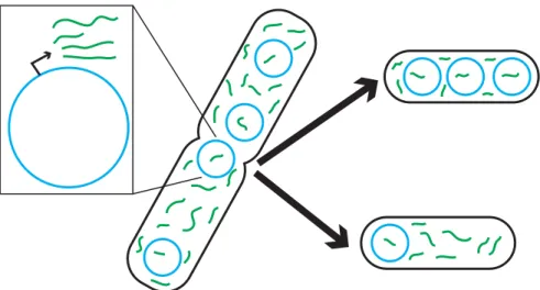
Figure 6: Plasmid transcription with partitioning. Each plasmid (blue) constitutively transcribes green RNA molecules. Both plasmids and RNA’s are partitioned between daughter cells during cell division.

A deterministic analysis of this plasmid replication rate can be performed. To do this analysis, assume that the cell volume is growing at a standard exponential rate with

˙

V =αV. (6)

Then, the dynamics of[P]can be computed. d[P] dt = d dt P V =V ˙ P−PV˙ V2 = 1 V2 P V β 1 +[_KP] −αP V ! = P V β 1 + [_KP] −α ! (7)

Setting the derivative equal to zero and solving gives the steady state value for the plasmid concentra-tion. [P]_eq=K _β α−1 (8) If volume is measured in units of cellular volume, then the average plasmid concentration can be thought as the steady state plasmid copy number. Note thatβ > αis required in order to have a non-negative steady state plasmid concentration. This is because the maximum rate of plasmid production must at least be able to keep up with the cell growth rate in order for the plasmid to be maintained.

Simulating plasmid replication and gene expression in single cells

Using the model of plasmid replication derived in the previous section, a model of plasmid replication com-bined with transcription can be used to compute the variability in mRNA levels between cells in a lineage simulation. In the model, there is one plasmid species, which replicates itself and also constitutively tran-scribes a mRNA. It is possible to look at the plasmid copy number and mRNA levels in a cell lineage over time as well as the plasmid copy number distribution across a population of cells at the end of the simu-lation. The full model used for producing the simulation is available in Appendix 2. However, the model is tuned to produce a mean plasmid concentration of 10 nM, and the cell division time is the same 33 minutes as in the previous section.

(12)

The simulation is performed for 500 minutes and the plasmid distribution is empirically calculated using a final population size of 2048 cells. The run time for this simulation to compute a total of 4095 cell traces is less than two seconds on a standard desktop computer without using parallel processing.

0 20 40 60 80 100 120 140 160 Time (min) 0 20 40 60 80 100 120 140 160 180 Concentration (nM)

RNA Concentration per Cell

0 20 40 60 80 100 120 140 160 Time (min) 0 50 100 150 200 250 300 Molecules

RNA Molecules per Cell

0 20 40 60 80 100 120 140 160 Time (min) 0 5 10 15 20 25 30 Molecules

Plasmids per Cell

0 5 10 15 20 25 30 35

Plasmid Copy Number

0.00 0.01 0.02 0.03 0.04 0.05 0.06 0.07 Empirical Densit y

Copy Number Distribution, N = 2048

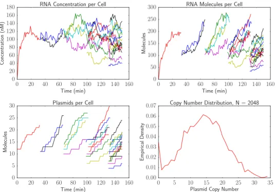
Figure 7: A simulation of plasmid replication and transcription over a cell lineage. The first three plots show trajectories of RNA and plasmid counts and concentrations over time. The last plot shows the distribution of plasmid copy number over 2048 cells at the end of the simulation.

As shown in Figure 7, the copy number at the end of the simulation has a wide distribution with a mean of about 15 copies per cell. This is expected because the mean concentration should be about 10 nM for the plasmid and the mean cell volume will be around 1.5 volume units. There is a slight peak in the distribution at a copy number of zero. This is because if a cell loses all its plasmids, it will continue dividing but its future descendants will never be able to recover the plasmid.

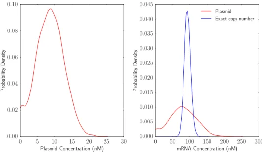
The distribution of plasmid and mRNA concentrations can also be plotted. In this case, the copy number is divided by the cell volume at the end of the simulation before plotting. The expected plasmid concentration is 10 nM and the expected mRNA concentration is 93.45 nM. The results can be seen in Figure 8.

The right panel of Figure 8 also shows a control where the plasmid concentration is assumed to be exactly controlled within the cell with no variability. In this case, the noise in mRNA expression is much smaller than in the case where the mRNA is expressed from the plasmid. The coefficient of variation in the plasmid based expression case is 0.55, while the coefficient of variation in the case with controlled copy number is0.10. The XML code for the model where the plasmid copy number is exactly controlled is available in Appendix 3.

Parameter inference for integrase dynamics

In the previous sections, we demonstrated the capabilities of the BioSCRAPE package for performing fast, flexible, and efficient simulations of biological circuits. In this section, we use the package’s parameter inference capabilities to do parameter inference for a model of integrase dynamics based onin vitro exper-imental data. We first start by giving background on integrase systems andin vitroprototyping of biological circuits. We then describe the experimental procedure and the experimental data collected. Finally, we

(13)

0 5 10 15 20 25 30 Plasmid Concentration (nM) 0.00 0.02 0.04 0.06 0.08 0.10 Probabilit y Densit y 0 50 100 150 200 250 300 mRNA Concentration (nM) 0.000 0.005 0.010 0.015 0.020 0.025 0.030 0.035 0.040 0.045 Probabilit y Densit y Plasmid Exact copy number

Figure 8: Distributions of plasmid and mRNA concentration across a cell lineage. The plasmid concentration is distributed around a mean of 10 nM. mRNA concentration is distributed around a mean of approximately 90 nM. The blue line shows the mRNA expression distribution if the plasmid concentration was exactly its mean value of 10 nM at all times.

introduce the model and perform parameter inference on the model for both simulated data as well as the actual experimental data.

Background and experimental design

Both serine integrase systems andin vitro prototyping using cell free extracts are common tools in syn-thetic biology. Serine integrases are proteins that can recognize and recombine two specific target DNA sequences (Smith and Thorpe, 2002; Groth and Calos, 2004). Depending on the original directionality of the target sites, the recombination causes the segment of DNA between the target sites to either be ex-cised or reversed. Figure 9B depicts the process by which four serine integrases bind to attB and attP DNA recognition sites and recombine them into attL and attR sites. In synthetic biology, this functionality has been leveraged to build synthetic gene circuits for state machines (Roquetet al, 2016), temporal event detection (Hsiaoet al, 2016), and rewritable memory (Bonnetet al, 2012). However, existing applications of integrases rely on their digital behavior over long time scales, and not much is known about the dynamics of their action upon DNA.

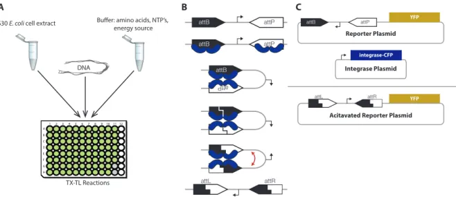
One way to assay the dynamics of integrase DNA recombination is to test an integrase system using TX-TL, an E. coli cell extract in vitro system for testing and protoyping synthetic gene circuits (Shin and Noireaux, 2012). Plasmid or linear DNA encoding the genes in a synthetic circuit can be added to a TX-TL master mix to prototype genetic circuits outside the cell as depicted in Figure 9A. In this case, we can create a simple synthetic circuit involving constitutive integrase production and reporter expression following DNA recombination to assay DNA recombination as a function of integrase levels. The circuit consists of two plasmids as shown in Figure 9C. On the first plasmid, the integrase plasmid, we constitutively express Bxb1, a commonly used serine integrase, as a part of a fusion protein in which Bxb1 is fused to CFP (cyan fluorescent protein). This allows us to use CFP fluorescence to measure the amount of Bxb1 present in the TX-TL reaction. The second plasmid is a reporter plasmid in which a promoter initially pointing away from a yellow fluorescent protein (YFP) gene can be reversed by integrase DNA recombination to point towards the YFP gene, which leads to production of YFP. Therefore, YFP expression can be used to infer when DNA recombination has occurred.

(14)

attB attP attB attP attB attP attL attR A B C D E F G H 1 2 3 4 5 6 7 8 9 10 11 12

S30 E. coli cell extract Buffer: amino acids, NTP’s,

energy source

DNA

TX-TL Reactions

integrase-CFP

Integrase Plasmid

attB attP YFP

Reporter Plasmid

YFP

Acitavated Reporter Plasmid attL attR

A B C

Figure 9: Testing serine integrase recombination dynamics using TX-TL. (A) The TX-TL system allows for prototyping synthetic circuitsin vitro by adding DNA to cell extract and buffer. (B) Four serine integrases recombine attB and attP DNA sites to form attL and attR sites while reversing the DNA segment between the sites. (C) A constitutive integrase expression plasmid expresses integrase fused to cyan fluorescent protein (CFP), which flips a promoter on a a reporter plasmid and leads to yellow fluorescent protein (YFP) expression.

Experimental Results

Using automated acoustic liquid handling, we varied the level of integrase plasmid and reporter plasmid between 0 and 1 nM across 100 different TX-TL reactions. Each reaction contained integrase and reporter plasmid both independently at one of five concentrations of 0 nM, 0.25 nM, 0.50 nM, 0.75 nM, or 1 nM. Therefore, there were 25 possible combinations of concentrations of the two plasmids. Four replicates were done for each combination of concentrations, yielding a total of 100 TX-TL reactions. The reactions were incubated at 37 degrees Celsius, and CFP and YFP fluorescence were collected every 5 minutes for each reaction using a plate reader. Using a previously performed calibration of fluorescence to concentration, we were able to convert the fluorescence measurements for CFP and YFP to actual concentrations in nM for each fluorescent protein. Notably, the CFP concentration allowed us to measure the concentration of Bxb1 integrase in the reaction.

In Figure 10A, the full experimental data is presented. The dots represent actual data points, and the solid lines represent the median of 4 replicates. In Figure 10B, the median expressions are plotted in columns corresponding to fixed levels of reporter plasmid. As expected, the first row shows that integrase expression increases as integrase plasmid is increased. It is also clear from the second row of Figure 10B that reporter expression generally begins sooner and ends at a higher level when there is more integrase expression.

Model of integrase recombination

In order to estimate parameters for the integrase data presented in the previous section, we needed a model of integrase recombination of DNA. As a first cut, we created a simple model of integrase dynamics consisting of three reactions: integrase production, DNA recombination, and reporter production. As TX-TL is a bulk environment, we chose to use a deterministic model for our system, which we easily set up using the BioSCRAPE package.

In Table 2, we describe the species in the model. These species are then used in the following set of ODE’s that describe the integrase recombination dynamics in the model.

(15)

0 50 100 150 200 0 50 100 150 200 250 CF P( nm ) 0 10 20 30 40 50 60 70 0 50 100 150 200 0 50 100 150 200 250 0 10 20 30 40 50 60 70 0 50 100 150 200 0 50 100 150 200 250 0 10 20 30 40 50 60 70 0 50 100 150 200 0 50 100 150 200 250 0 10 20 30 40 50 60 70 0 50 100 150 200 0 50 100 150 200 250 0 10 20 30 40 50 60 70 YF P( nm ) 0 50 100 150 200 0 50 100 150 200 250 CF P( nm ) 0 10 20 30 40 50 60 70 0 50 100 150 200 0 50 100 150 200 250 0 10 20 30 40 50 60 70 0 50 100 150 200 0 50 100 150 200 250 0 10 20 30 40 50 60 70 0 50 100 150 200 0 50 100 150 200 250 0 10 20 30 40 50 60 70 0 50 100 150 200 0 50 100 150 200 250 0 10 20 30 40 50 60 70 YF P( nm ) 0 50 100 150 200 0 50 100 150 200 250 CF P( nm ) 0 10 20 30 40 50 60 70 0 50 100 150 200 0 50 100 150 200 250 0 10 20 30 40 50 60 70 0 50 100 150 200 0 50 100 150 200 250 0 10 20 30 40 50 60 70 0 50 100 150 200 0 50 100 150 200 250 0 10 20 30 40 50 60 70 0 50 100 150 200 0 50 100 150 200 250 0 10 20 30 40 50 60 70 YF P( nm ) 0 50 100 150 200 0 50 100 150 200 250 CF P( nm ) 0 10 20 30 40 50 60 70 0 50 100 150 200 0 50 100 150 200 250 0 10 20 30 40 50 60 70 0 50 100 150 200 0 50 100 150 200 250 0 10 20 30 40 50 60 70 0 50 100 150 200 0 50 100 150 200 250 0 10 20 30 40 50 60 70 0 50 100 150 200 0 50 100 150 200 250 0 10 20 30 40 50 60 70 YF P( nm ) 0 50 100 150 200 Time (min) 0 50 100 150 200 250 CF P( nm ) 0 10 20 30 40 50 60 70 0 50 100 150 200 Time (min) 0 50 100 150 200 250 0 10 20 30 40 50 60 70 0 50 100 150 200 Time (min) 0 50 100 150 200 250 0 10 20 30 40 50 60 70 0 50 100 150 200 Time (min) 0 50 100 150 200 250 0 10 20 30 40 50 60 70 0 50 100 150 200 Time (min) 0 50 100 150 200 250 0 10 20 30 40 50 60 70 YF P( nm ) integrase-CFP Integrase Plasmid 0 nM

A

B

0 nM 1 nM 1 nM

attB attP YFP

Reporter Plasmid 0 nM int. plasmid 0.25 nM int. plasmid 0.50 nM int. plasmid 0.75 nM int. plasmid 1.00 nM int. plasmid 0 100 100 200 200 0 20 40 0 0 100 200 0 100 200 0 100 200 0 100 200 CFP (nM) Time (min)

0.00 nM Reporter 0.25 nM Reporter 0.50 nM Reporter 0.75 nM Reporter 1.00 nM Reporter

Time (min) Time (min) Time (min) Time (min) YFP (nM)

Figure 10: Experimental results for integrase testing. (A) Both integrase plasmid and reporter plasmid were varied from 0 to 1 nM and fluorescence data was collected for 4 hours. The dots are actual data points and the solid lines are the median of 4 replicates. (B) The median fluorescence trajectories plotted for fixed amounts of reporter plasmid. The reporter turns on sooner when more integrase is expressed.

˙ I=kIIpl ˙ A=f R I Kf n 1 +_KI f n ˙ R=A ˙ Y =kYA (9)

Equation 9 contains the ODE’s for the simple model. Integrase is produced at a constitutive rate, where Ipl is the concentration of integrase plasmid and varies across experiments. The conversion of reporter

(16)

Table 2: Species and parameters in the simple model of integrase recombination

Variable Species

I Integrase-CFP (nM)

A Activated reporter plasmid (nM) R Unactivated reporter plasmid (nM) Y YFP fluorescent reporter (nM) I_pl Integrase plasmid (nM)

Parameter Description

kI Rate of integrase production (nM integrase per minute per nM integrase plasmid)

f Maximum rate of integrase flipping of DNA (nM activated plasmid per nM reporter plasmid per minute) Kf Hill threshold for integrase activation (nM integrase)

n Hill coefficient

kY Rate of reporter production (nM reporter per minute per nM activated plasmid)

and activation threshold for the integrases in a simple way. We also assume that the DNA recombination reaction is first order in reporter plasmid. Finally, we assume that reporter is produced at a rate proportional to the amount of activated reporter plasmid. While varying the integrase plasmid changes the value ofIpl

in the model, varying the reporter plasmid changes the initial condition forR.

0 nM int. plasmid 0.25 nM int. plasmid 0.50 nM int. plasmid 0.75 nM int. plasmid 1.00 nM int. plasmid 0 100 100 200 200 0 20 40 0 0 100 200 0 100 200 0 100 200 0 100 200 CFP (nM) Time (min)

0.00 nM Reporter 0.25 nM Reporter 0.50 nM Reporter 0.75 nM Reporter 1.00 nM Reporter

Time (min) Time (min) Time (min) Time (min) YFP (nM)

Figure 11: Simulated version of Figure 10B using the model.

Using representative values for the model, we created a simulated version of Figure 10B using the model. The plot is given in Figure 11, and there are some qualitative differences between integrase expres-sion in the simulations and in the experimental data. Namely, while in the model the expresexpres-sion of integrase increases linearly with a slope proportional to the amount of integrase plasmid, in the experimental data, integrase expression only increases after a delay and then levels off after about two hours. This behav-ior is common in cell free extracts due to depletion of resources, and this effect should be included in a future more detailed model of the system. The full XML model for integrase dynamics and the numerical parameter values used in simulations are included in Appendix 4.

(17)

Parameter inference for integrase dynamics

Using the model given in Equation 9, we attempted to perform parameter inference using BioSCRAPE to fit the model parameters to both the simulated data from Figure 11 as well as the experimental median data from Figure 10B. Fitting the model to simulated data was a computational test of the identifiability of the model from the collected data. If a simulated version of the data were uninformative about parameter values in the models, then the real data would not be informative about the parameters either.

The parameter inference code in BioSCRAPE allows a user to enter a set of experiments into a likelihood function as well as specify a prior distribution on parameters. This information is then sent to an off the shelf ensemble Markov chain Monte Carlo package that generally works well on parameter inference problems (Goodman and Weare, 2010; Foreman-Mackeyet al, 2013).

-10 0 10 Posterior Density

A

-10 0 10 -1.0 0.5 2.5 -10 0 10 -10 0 10 -10 0 10 Posterior Density

B

-10 0 10 -1.0 0.5 2.5 -10 0 10 -10 0 10

Figure 12: Posterior parameter estimates from MCMC. (A) Parameter distributions (blue) for the simulated data are strongly peaked around the true parameter values (green). (B) Parameter distributions for the experimental data from Figure 10B.

Figure 12 contains the posterior distributions for the parameters obtained after performing parameter estimation. From Figure 12A, it is clear that for simulated data, the true parameters are clearly identifiable from the simulated data. This suggests that the collected data should be informative about the parameter values.

Figure 12B contains the posterior parameter estimates from parameter estimation on the experimental data. In this case, most of the parameter distributions are again strongly peaked, except for the integrase throughput rate f. However, it is notable that the distribution forf is negligible forf < 1 and essentially uniform for f > 1. This suggests that the integrase throughput is much faster than gene expression. Because we are dependent on gene expression of the fluorescent reporter to infer when DNA recombination occurs, this posterior distribution suggests that we cannot exactly identify how fast the DNA recombination is, because the DNA recombination occurs much faster than the following gene expression.

(18)

Table 3: Estimates for Hill coefficient and activation threshold

Variable Median 16th to 84th percentile interval

Hill coefficientn 5.4 (4.4,5.8) Activation thresholdKf (nM) 45 (22,91)

The other parameters we are interested in are the Hill coefficient and activation threshold for integrase activity. These estimates are given in Table 3 along with their confidence intervals based on the posterior distributions. We found that Hill activation threshold was on the order of tens of nanomolar, which would correspond to anin vivo concentration of a few dozen molecules per cell. We found a Hill coefficient of 5.4, which was surprising, because four integrases combine to recombine DNA, so we expected the Hill coefficient to be no more than 4.

Discussion

The advent of increased computational resources and high throughput data collection for biological circuits has made quantitative modeling and parameter estimation for biological circuits more feasible. Since the most attractive parameter estimation techniques rely on Bayesian inference and Markov chain Monte Carlo (MCMC), it is important to have a simulator that can perform fast forward simulations of the model. Addition-ally, this simulator must be able to produce the same types of data that are observed in standard biological assays such as flow cytometry or fluorescence microscopy. Also, as models often need to be tweaked to fit the data, it should be easy to change the model or the way the model is simulated (e.g. switching from a deterministic to a stochastic simulation).

The BioSCRAPE package addresses all of these issues. The flexible XML based language for model specification allows a user to easily make modifications to a biological circuit model by simply spending a minute editing a text file. The flexible Python based library for performing simulations allows for easily swap-ping between deterministic and stochastic simulations as well as consideration of other common effects in biological circuits such as cell growth and division and delays. Finally, because this package is written in Cython, its speed is comparable to the speed obtained using C code.

Performing simulations that incorporate effects like cell growth and division and delay can provide insight into the behavior of biological circuits. For example, in this paper, it is demonstrated that in an exponentially dividing colony of cells, delays in gene expression can lead to a lower steady state protein level. This has implications for selection of fluorescent proteins for use in exponentially growing colonies. This paper also demonstrates how transcribing a gene off a plasmid with copy number fluctuations will lead to more noise in expression than if the copy number of the plasmid were controlled exactly.

However, the ultimate aim of this package is to provide tools for doing parameter estimation for synthetic and systems biology. Here, we demonstrated the use of the BioSCRAPE package to perform parameter estimation for both simulated and experimental data for integrase recombination dynamics in the TX-TL cell

freein vitro system. As a result of this demonstration, we were able to estimate parameters for both the

activation threshold and cooperativity of integrases that may be relevant for synthetic circuit design. The fast simulators presented here will be the computational workhorse for more complex MCMC schemes for performing parameter inference for stochastic models of synthetic gene circuits. A future update to this report and the code will include inference methods and an experimental demonstration for a stochastic model.

Acknowledgements

The authors would like to acknowledge Marcella M. Gomez, Noah Olsman, Vipul Singhal, and Eduardo Sontag for helpful discussions and testing of the software.

(19)

The project depicted is sponsored by the Defense Advanced Research Projects Agency (Agreement HR0011-17-2-0008). The content of the information does not necessarily reflect the position or the policy of the Government, and no official endorsement should be inferred.

Author Contributions

AS conceived of BioSCRAPE, wrote the software, developed the examples and code for modeling integrase dynamics, and wrote the technical report with feedback from RMM and VH.

VH conceived of performing integrase characterization in TX-TL and collected the experimental data. VH also provided feedback on data analysis, parameter estimation, and the technical report.

RMM provided project supervision and feedback on the technical report.

Appendix 1: Full XML Model for Simple Gene Expression

<model>

</reaction>

</reaction>

</reaction>

</reaction>

(20)

Appendix 2: Full XML Model for Plasmid Replication and

Transcrip-tion

<model>

</reaction>

</reaction>

Appendix 3: Full XML Model for Transcription with Exactly Controlled

Copy Number

<model>

</reaction>

(21)

Appendix 4: Full XML Model for Integrase Dynamics

<model>

References

Behnel S, Bradshaw R, Citro C, Dalcin L, Seljebotn D, Smith K (2011) Cython: The Best of Both Worlds.

Computing in Science Engineering13: 31 –39

Bonnet J, Subsoontorn P, Endy D (2012) Rewritable digital data storage in live cells via engineered control of recombination directionality.Proceedings of the National Academy of Sciences of the United States of

America109: 8884–8889

Brendel V, Perelson AS (1993) Quantitative Model of ColE1 Plasmid Copy Number Control. Journal of

(22)

Del Vecchio D, Murray RM (2014)Biomolecular Feedback Systems. Princeton University Press Eldar A, Elowitz MB (2010) Functional roles for noise in genetic circuits.Nature467: 167–173

Elowitz MB, Levine AJ, Siggia ED, Swain PS (2002) Stochastic Gene Expression in a Single Cell.Science 297: 1183–1186

Foreman-Mackey D, Hogg DW, Lang D, Goodman J (2013) emcee: The MCMC Hammer.arXiv 125: 306 Gillespie DT (1977) Exact stochastic simulation of coupled chemical reactions. The Journal of Physical

Chemistry81: 2340–2361

Golightly A, Wilkinson DJ (2011) Bayesian parameter inference for stochastic biochemical network models using particle Markov chain Monte Carlo.Interface Focus

Gomez MM, Sadeghpour M, Bennett MR, Orosz G, Murray RM (2016) Stability of Systems with Stochastic Delays and Applications to Genetic Regulatory Networks.SIAM Journal on Applied Dynamical Systems 15: 1844–1873

Goodman J, Weare J (2010) Ensemble Samplers with Affine Invariance.Communications in Applied

Math-ematics and Computational Science5: 65–80

Groth AC, Calos MP (2004) Phage Integrases: Biology and Applications.Journal of Molecular Biology 335: 667 – 678

Hsiao V, Hori Y, Rothemund PW, Murray RM (2016) A population-based temporal logic gate for timing and recording chemical events.Molecular Systems Biology 12: 869

Hucka M, Finney A, Sauro HM, Bolouri H, Doyle JC, Kitano H, Arkin AP, Bornstein BJ, Bray D, Cornish-Bowden A,et al (2003) The systems biology markup language (SBML): a medium for representation and exchange of biochemical network models.Bioinformatics19: 524–531

Huh D, Paulsson J (2011) Random partitioning of molecules at cell division.Proceedings of the National

Academy of Sciences108: 15004–15009

Komorowski M, FinkenstÃd’dt B, Harper CV, Rand DA (2009) Bayesian inference of biochemical kinetic parameters using the linear noise approximation.BMC Bioinformatics10: 343

Maarleveld TR, Olivier BG, Bruggeman FJ (2013) StochPy: A Comprehensive, User-Friendly Tool for Sim-ulating Stochastic Biological Processes.PLOS ONE 8: 1–10

MATLAB (2016)version 9.0.0 (R2016a). Natick, Massachusetts: The MathWorks Inc.

Moore SJ, MacDonald JT, Weinecke S, Kylilis N, Polizzi KM, Biedendieck R, Freemont PS (2016) Prototyp-ing of Bacillus megaterium genetic elements through automated cell-free characterization and Bayesian modelling.bioRxiv

Roquet N, Soleimany AP, Ferris AC, Aaronson S, Lu TK (2016) Synthetic recombinase-based state ma-chines in living cells.Science353: aad8559

Sachs K, Perez O, Pe’er D, Lauffenburger DA, Nolan GP (2005) Causal Protein-Signaling Networks Derived from Multiparameter Single-Cell Data.Science308: 523–529

Shin J, Noireaux V (2012) An E. coli Cell-Free Expression Toolbox: Application to Synthetic Gene Circuits and Artificial Cells.ACS Synthetic Biology 1: 29–41

Smith MCM, Thorpe HM (2002) Diversity in the serine recombinases.Molecular Microbiology44: 299–307 Stricker J, Cookson S, Bennett MR, Mather WH, Tsimring LS, Hasty J (2008) A fast, robust and tunable

(23)

Young JW, Locke JCW, Altinok A, Rosenfeld N, Bacarian T, Swain PS, Mjolsness E, Elowitz MB (2012) Measuring single-cell gene expression dynamics in bacteria using fluorescence time-lapse microscopy.

Nature Protocols7: 80–88

Zechner C, Ruess J, Krenn P, Pelet S, Peter M, Lygeros J, Koeppl H (2012) Moment-based inference predicts bimodality in transient gene expression.Proceedings of the National Academy of Sciences109: 8340–8345

. CC-BY-NC-ND 4.0 International license

. http://dx.doi.org/10.1101/121152

https://github.com/ananswam/bioscrape_distr.