ISSN: 2038-7296 POLIS Working Papers [Online]
Dipartimento di Politiche Pubbliche e Scelte Collettive – POLIS
Department of Public Policy and Public Choice – POLIS
POLIS Working Papers n. 180 February 2011
Microcredit and poverty.
An overview of the principal statistical
methods used to measure the program net impacts
Cristina Elisa Orso
UNIVERSITA’ DEL PIEMONTE ORIENTALE “Amedeo Avogadro” ALESSANDRIA Periodico mensile on-line "POLIS Working Papers" - Iscrizione n.591 del 12/05/2006 - Tribunale di Alessandria
Microcredit and Poverty. An
overview of the principal statistical
methods used to measure the
program net impacts.
Cristina Elisa Orso
Abstract
The purpose of this paper is to examine di¤erent economet-ric approaches aiming to evaluate the impact of microcredit on poverty. Starting with a brief description of microcredit and the most common kinds of statistical biases connected to these stud-ies, I describe the principal characteristics of Non-Randomized and Randomized approaches, in order to highlight strengths and weaknesses concerning the application of such methodologies.
JEL-Classi…cation: C54, C58.
Keywords: Microcredit, poverty, program impact, random-ized approach, non-randomrandom-ized approach.
Ph.D. Student in "Economic Policy", Department of Economic and Social Sci-ences, Catholic University, Piacenza. E-mail: [email protected]
1.
Introduction
Scienti…c testing of the net impact of microcredit is very di¢ cult. It is possible to identify a speci…c question which represents the core of every serious impact study: if we …nd out that people who have obtained loans are doing better than those who haven’t, does it necessarily mean that receiving loans caused the positive change? In other words, the problem is to understand how outcomes have changed with the program compared to what would have happened without the program implementation.
The most important challenge, in this particular context, has been to determine a control group for comparison; it is very hard to identify a group of people who are like the program participants in all relevant features apart from not having received funds. The critical issue to evaluate how micro…nance works is the measure-ment of the net e¤ects caused by the programs.
As outlined by Armendàriz, Morduch (2010), the …rst contribu-tions of microcredit impact literature mainly concerned non-experimental methods. In this context, researchers use treatment and con-trol groups, but do not randomly assign subjects to the groups. The critical point in such studies is to establish causality relation-ships. Moreover, biases from omitted variables, non-random pro-gram placement, client selection and self selection, and attrition lead to important estimation problems (Karlan, 2001).
Some kinds of biases can be reduced by using longitudinal data. The e¤ects of non-random participation and non-random program placement, under speci…c assumptions, can be mitigated by the implementation of this strategy. But if there are unobservable vari-ables that change over time, attributes hard to measure such as entrepreneurial organization and business skills are probably cor-related with participation status. The most popular longitudinal studies have been sponsored by USAID in the second part of 1990s. Researchers investigated net impacts on members of three di¤erent institutions: a microlender organization operating in the informal sector (SEWA) located in Ahmedabad (India), an ACCION In-ternational a¢ liate (Mibanco) situated in Peru and the Zambuko Trust in Zimbabwe. The sample households were observed a …rst time to collect baseline data, and then, after two years, they were resurveyed (Armendàriz, Morduch, 2010).
Some empirical work is based on household surveys from the World Bank and the Bangladesh Institute of Development Studies in
Bangladesh. The studies that exercise the most in‡uence on the research community are Pitt and Khander (1998) and Khander (2005). As regards PK approach, they use cross-section data (from the three seasonal rounds in 1991/1992), while Khander takes into account the panel dimension of the data set (he also uses the 1999 round) in order to strengthen identi…cation. To follow, many other studies are based on this data set. We report, for instance, Khan-der (1996, 2000), Pitt et al. (1999), McKernan (2002), Pitt and Khander (2002), Pitt et al. (2003), Menon (2005), and Pitt, Khan-der and Cartwright (2006).1
Concerning experimental approach, randomized controlled trials (RCTs) , when done correctly, can really provide credible and transparent estimates in di¢ cult contexts. Such approach consists of giving loans to a subgroup randomly drawn from the population ( for instance through a random algorithm to select people from a list), while the other subgroup, also randomly selected, will not ob-tain any funds.Using randomized approach, the di¤erence in terms of average outcome between the two distinct groups represents a good estimate of the program’s average impact. Under determinate assumptions, the result can be interpreted as the causal impact of microcredit introduction.2
However, we must notice that it is an average impact; therefore, if half of the participants gains by 100 percent while the other half loses by 100 percent, the average impact will be zero. In a similar context, zero is a clean estimate of the average impact, but it doesn’t give us any relevant information about an individual’s performance.
In order to obtain credible estimates, it is important that neither agreement to participate in the experiment nor the tendency to drop out are systematically related to outcomes of interest. Randomization approaches also have limits: few published exper-imental studies of micro…nance have been able to highlight short-term results only.
Banerjee et al.(2009) and Karlan and Zinman (2009) looked at mi-crocredit participants over a short period of time ( 12-18 months). They didn’t …nd any kind of improvement in household income or consumption, but both the studies showed some other bene…ts.
1For a more complete literature review, see Armendàriz, Morduch, 2010.
2Because of RCTs implementation, loans represent the only ex-ante di¤erence
The former concerns a randomized evaluation on the community-level impact of the introduction of new branches of a local micro…-nance bank. The baseline sample was randomly selected from ur-ban Hyderabad (India) for the opening of new micro…nance branches. Before new institutions opened, 69 percent of the households had at least one outstanding loan from informal channels (moneylenders, family, friends). The authors found that the new branches settle-ment caused, in the interested areas, more new business openings, higher purchases of durable goods and relevant pro…ts in existing business activities. However, it’s important to note that the main e¤ects concern target households starting new businesses, and the authors can’t tell if the funds are actually invested in business activities or not.
Interestingly, Dupas and Robinson (2009) conducted a randomized …eld experiment in Kenya that found short-term welfare improve-ment regarding micro-savings, not microcredit.
They gave interest-free savings accounts in a local micro…nance institution to a random sample of small entrepreneurs; these ac-counts did not pay interest and charged withdrawal fees, but they represented the only opportunity for formal savings in the area. The results suggested wide variation in the intensity of formal ac-count usage. Some microentrepreneurs did not accept the pro-posal, and many accepted without using the account e¤ectively; roughly 50 percent of those with accounts used them only rarely, and only a small minority used them frequently.
Clients of this service increased their investment and daily expendi-tures for women, but there was no evidence in terms of men impact. However, this study presents a few shortcomings: …rst, the random sample is small (185 microentrepreneurs) and only few clients used the account frequently. Moreover, the target area of experiment was limited to a single site and to a single micro…nance bank . Karlan and Zinman (2008) conducted a randomized experiment in South Africa. The authors asked loan o¢ cers of a local lender to revalue and accept applicants for a microloan from a set who were initially refused but who got just below the cutt-o¤.
Many applicants who were reconsidered (but not all) showed in-come improvements and a more positive outlook on the future. Despite of a micro-entrepreneur set rejected and not reconsidered, they registered a higher level of stress and depression.
The results of this study can’t generalize to other micro…nance contexts, because the loans were consumer loans, not typically used for investments in business activities. In addition, applicants were not very poor, and interest rates were higher than those applied by typical micro…nance institutions (Rosenberg, 2010).
The remainder of this paper is organized as follows. The next section provides a brief description of microcredit and its princi-pal objectives, among which poverty alleviation. Section 3 gives a sketchy outline of the problems arising from reverse causation and selection bias in order to discuss about the econometric method-ologies to use. Section 4 and section 5 respectively describe the two distinct empirical approaches, examining the results reached in both …elds on the basis of recent literature. Section 6 com-pares randomized and non-randomized strategies. The last section concludes with a discussion of the principal impact issues.
2.
De…nition and aims of Microcredit
According to its basic de…nition, microcredit involves small loans to poor people for self employment projects that produce income, allowing them to care for themselves and their families.3 These
individuals, also called "unbankable", lack any kind of economic collateral and a veri…able (and valuable) credit history to o¤er a traditional bank. Hence, they cannot meet the basic quali…cations required to access formal credit. Microcredit can be considered a …eld of micro…nance, which embraces the provision of a wider range of …nancial services designed for the very poor. As highlighted by Armendariz, Morduch (2010), recently the terms microcredit and
micro…nance have often been used interchangeably even if they
show some remarkable di¤erences. The original focus on microcre-dit mainly concerned poverty reduction and social change, and the most important institutions involved were NGOs. Then, the shift
tomicro…nance arose from the growing need of poor households for
a broader range of …nancial services (like savings) and not exclu-sively credit for entrepreneurial activities. As a result, this lexical transition has produced an orientation change, toward less poor people and toward a di¤erent kinds of organizations, commercially oriented and with strong …nancial regulations.
The term microcredit is often used in distinct contexts (rural credit, agricultural credit, consumer credit, etc.) with di¤erent implica-tions. In order to clarify the target and the speci…c objectives of
the programmes, we introduce a broader classi…cation to identify the various categories.
On the basis of Yunus taxonomy4, it is possible to identify …ve di¤erent kinds of microcredit:
- Traditional informal microcredit (moneylender’s credit, pawn shops, loans from friends and relatives, consumer credit in infor-mal markets). Amongst those of that sector local moneylenders are an important source of credit to those borrowers usually refused by most …nancial institutions because of their particular economic conditions. Low income and lack of collateral and stable employ-ment do not make borrowers creditworthy in the eyes of traditional banks. Moneylenders are better at serving clients neglected by the formal sector because they have a considerable market knowledge and lower transaction costs. At the same time, they can easily monitor borrower behaviour because of their proximity to the client and reliable information about his or her status. Poor people turn to moneylenders mainly for consumer loans or to cope with emer-gencies like health problems or to pay for high outlay connected with education, wedding, funerals, and so on. Hence this source of credit cannot be considered a valid engine of inclusion and local growth.
- Microcredit based on traditional informal groups (tontine, ROSCA). Tontine can be compared to our life insurance. The basic scheme is simple. Each participant contributes a sum of money to the ton-tine and, then, he receives an annual dividend on his investment. When each participant dies, his or her share is reallocated among the surviving subscribers, until only one investor survives. ROSCA (Rotating Savings and Credit Association) consists of a group of in-dividuals who agree to meet for a speci…c period of time in order to save and borrow money from a common "pot", usually allocated to one member of the group (who changes each period). Both kinds of microcredit pursue partially di¤erent objectives compared to modern microcredit. The aim of tontine concerns insurance, while ROSCAs …nance consumer credit (Armendàriz-Morduch, 2010). - Microcredit through traditional banks, generally specialised in speci…c investment sectors (agricultural credit, livestock credit, …sheries credit, handloom credit, etc.).
- Cooperative microcredit and rural credit through specialised banks.
- Modern microcredit (Grameen credit, bank-ONGs partnership based microcredit and consumer microcredit). Small loans typi-cally designed for low-income clients who traditionally lack access to commercial banking for several reasons (absence of collateral, informal employment, unveri…able credit history, high transaction costs). This kind of credit allows poor people to start new en-trepreneurial activities, expand existing businesses, to cope with shocks due to adverse climatic conditions and illness, and smooth out consumption.
Concerning the last category of microcredit, three models for lend-ing have become globally popular: village banking,solidarity groups, and individual lending. The choice of lending technology relies on the speci…c characteristics and needs of the target areas.
Thevillage banking approach is most similar to the old cooperative
credit movement. This method was innovated by FINCA Interna-tional founder, John Hatch. A village bank is an informal self-help support group of 20-30 participants ( predominantly women). The …rst loan comes from an institution like MFI or NGO, then follow-ing deposits come from individual savfollow-ings amounts in group funds. For example, if the …rst loan is $ 50 and the participant saves in the same period $ 10, the second loan will be equal to $ 60. The length of the loan cycle is 4-6 months5. SHGs (self-help groups)
have dominated the micro…nance landscape especially in India. These involve small groups of 10-20 members that collect savings from their participants and, at the same time, provide them with loans. The members are jointly and severally liable for the funds obtained within the group itself (Nair, 2005).
Solidarity groups is a lending mechanism which allows a group of
people to provide collateral through a group repayment pledge6.Usually
borrower groups are made up of three to seven members, most com-monly …ve7, and the patterns of disbursements and repayments is 5For detailed information, see:
http://en.wikipedia.org/wiki/Village_Banking
6http://www.accion.org/ Group_Lending
7Five is the right size of a Grameen group. Grameen Bank (or Rural Bank)
was started by Muhammad Yunus, a Professor of the University of Chittagong (Bangladesh) in 1976. The bank mainly targeted rural women for its credit pro-grammes. It introduced group lending strategy to make credit available to the poor, usually denied by commercial loans because of the lack of physical collateral. The income-generation also aims to empower the women and increases their participa-tion in household decisions. For more details about its "mission" and history, see Armendàriz, Morduch, 2010, chapter 4.
regimented. According to the Grameen model, payments start im-mediately after disbursement every week. In practice, the …rst two participants take their loans and begin with repayment, then two more, and …nally the …fth. The eligibility to further and larger amounts of funds is subject to the repayment of all group loans. Each borrower is responsible for the repayment of all the other loans within the group (joint liability). The advantages of this methodology concern lenders and customers. First, it is conve-nient for villagers because the bank comes to them (as in the cases of ROSCAs and local moneylenders), avoiding logistic and admin-istrative problems. At the same time, for the lender, transaction costs connected to loan disbursement are considerably reduced. Although this methods boasts some evident strengths, the higher likelihood of group failure in the event of a single default, the huge training costs and the greater …nancial responsibility for others in a group have to be taken into consideration when looking into its implementation (Armendàriz, Morduch, 2010).
The case of individual lending substantially di¤ers from previous approaches. Typically, microcredit is associated with group struc-tures (solidarity groups or village banks). Whilst the …rst two lending models serve the poorest, individual lending serves less poor clients. This targeting choice arises from the high costs of underwriting new loans, monitoring behaviour and repayment of disbursed funds, and enforcing repayment process. Group lend-ing strategies, as mentioned above, shift much of the responsibil-ity onto borrowers, while lending to individuals involves (for the MFI) managing these costs directly. Interestingly, however, some microcredit institutions do not o¤er group but individual loans. BDB (Bank Dagang Bali) and BRI (Bank Rakyat Indonesia), two Indonesian private banks, are revealing examples of individual mi-cro…nance8. As in conventional lending, loan o¢ cers take collateral and collect information from credit bureaus, require pledges of ti-tle to land or to other property. Sometimes, the individual lending is a part of a larger "credit plus" program, where other particu-lar kinds of services (such as skill development, education, health, etc.) are provided.
To sum up, it is possible to highlight some general key objectives of the microcredit programmes:
(a) to provide small loans to poor people at lower cost than infor-mal sources;
(b) to avoid exploitation of the poor due to the growth of informal credit channels;
(c) to reach the "unbankable" that cannot be …nanced by tradi-tional banks (because of the lack of collateral);
(d) to empower women both within the household (as decision makers) and in society (through active economic and political par-ticipation);
(e) to improve employment opportunities;
(f) to reduce poverty, increase growth and improve the living con-ditions on sustainable perspectives.
As regards the last point, microcredit is gaining importance as an e¤ective tool of poverty alleviation. Impact evaluations aim to investigate the role of credit access in terms of poverty reduc-tion. Although some interesting research9 analyzes the e¤ects of
microcredit programmes through a multidimensional poverty per-spective10, …nancial outcomes remain the core matter in many
rel-evant impact studies. The lack of reliable data and the selection problems connected with empirical evaluations represent a serious complication to estimate microcredit consequences.
3.
Econometric impact evaluations: selection bias and
causal-ity
Microcredit and the other micro…nance services can a¤ect individ-uals and households in many di¤erent ways. The …rst question
9Karlan, Zinman (2010) conducted an interesting study using an experimental
approach. They measure the impact of microcredit programmes (in Manila) also in terms of subjective well-being using indicators such as life satisfaction, job satisfac-tion, decision making power, optimism, etc. In addisatisfac-tion, the authors investigated the treatment e¤ects on di¤erent kinds of human capital.
As mentioned in the introduction, Karlan and Zinman (2008) created another inter-esting experiment aiming to estimate impact e¤ects of microcredit in South Africa. In addition to …nancial impact measures (such as income and consumption), they consider particular types of indices concerning health aspects (physical and mental health index) and decision- making process, optimism, and position in the commu-nity socio-economic ladder (this information comes from subjective perceptions of sample households).
10Multidimensional poverty involves a group of deprivations that cannot be
ade-quately expressed as income insu¢ ciency. It refers to speci…c composite measures, such as the Human Poverty Index, that accounts for well-being indicators (like a decent standard of living, a long and healthy life, knowledge). For more details, see Tsui, 2002.
that researchers have to ask is the following: what are we trying to measure?
Concerning the impact of microcredit, we distinguish between two di¤erent e¤ects:
(a) an income e¤ect, that makes households wealthier and pushes up consumption levels (it can also increase the demand for children, health, children’s education, spare time);
(b) a substitution e¤ect, which may counterbalance the income e¤ect. In fact, with increased female employment rates, hours spent raising o¤spring can be costlier in terms of foregone income, driving birth levels down.
But increasing income and consumption are not the only metric of judgement of microcredit impact.
As argued in a interesting book, Portfolios of the poor: How the
World’s Poor live on $2 a day (Collins, Morduch, Rutherford, and
Ruthven, 2009), the poor tend to use credit and savings not only in order to smooth consumption, but also to cope with emergen-cies like health problems and pay for expensive services such as education, weddings, or funerals.
A lot of studies have looked at the experience of people who have obtained microloans.
In order to have a clean estimate of evaluating impacts, the statis-tical problem is to separate out the causal role of microcredit pro-gram. In other words, it is necessary to gauge microcredit e¤ects eliminating the various reverse causation and selection biases. As regardscausality, researchers have to answer fundamental ques-tions. For example, if they note that wealthier households have larger loans, they have to ask if the loans enrich the households or do richer households merely have less di¢ culty in accessing credit, without a substantial increase in their productivity (Armendàriz, Morduch, 2010).
The challenge has been to identify an appropriate control group for comparison; we have to ask if changements as new business, new saving accounts, further education for children, etc. are due to the program implementation or would have happened also without microcredit introduction.
We can summarize the e¤ect produced by a speci…c treatment (T) on a characteristic Y ( in order to understand whether and in
what size the treatment may be considered a determinant factor of Y) as follows11:
=E(Y1
i =Ti = 1) E(Yi0=Ti = 0)12 (1)
In this context, the causal e¤ect is measured as the di¤erence be-tween the outcome that would be observed if unit i received the treatment (E(Y1
i =Ti = 1)), and the outcome of receiving no
treat-ment of any kind (E(Y0
i =Ti = 0)).
Econometric methods attempting to estimate how much of the distinct outcomes between treatment and control groups attribut-able to the program are a crucial tool in microcredit interventions, especially in non-experimental settings. The question that every evaluation seeks to solve is how would partecipants have done in absence of intervention. As well argued in Holland (1986), the fun-damental problem of causal inference concerns the impossibility of evaluating, at the same time, treatment and no treatment, that is Ti = 1 and Ti = 0; obviously, it is not possible observing the
results obtained on the same unit from the two di¤erent situations ( E(Yi1=Ti = 1) and E(Yi0=Ti = 0)) in order to gauge the causal
e¤ect ofT on Y.
Di¤erent counterfactual statistical estimation methodologies have to be implemented on the basis of the speci…c evaluation context. In particular, we imagine to have to measure the causal impact of microcredit on borrower income. The income level can be at-tributed to di¤erent kinds of sources: measurable attributes, for example, like job, business, pension, age, education and experi-ence, that are generally available.
But another category of personal characteristics is hard to measure, for instance organizational ability, entrepreneurial skills, access to valuable social networks. In this latter category, we include eco-nomic shocks, and other types of casual events that could a¤ect household outcomes (Armendàriz, Morduch, 2010).
In addition, a further set of attributes may be useful in order to estimate microcredit impact, such as village size, or the existence of scale economies related to speci…c production (actually, this kind of information is measurable but not gathered in surveys).
11See Du‡o, Glennetster, and Kremer (2007)
12where " " represents the measure of the impact,E(Y1
i /Ti= 1) is the expected
value of the outcome variable observed after treatment on target units, while E( Y0 i /Ti= 0) is the expected value after program implementation on control group.
Estimating microcredit impact implies separating out its role from the roles of all these di¤erent attributes.
Bank o¢ cers work hard to screen potential ranges of customers, and calculate the optimal locations for new branches; loans are thought to attract the most gifted individuals, who choose to parte-cipate or not in a microcredit program on the basis of personal and strategic reasons (in particular, on the basis of perceived returns). If target clients are wealthier and more productive than the non-treated group, it could be attributed to the strategic placement of the intervention, not to the active role of the micro…nance institu-tion in making these condiinstitu-tions. Hence, a high correlainstitu-tion between microcredit participation and, for example, the variables age and entrepreneurial ability is very probable.
In this context, if investigators manage measurable attributes (like age), there are simple strategies in order to control for age-related issues, but when there are typical unmeasurable attributes, such as entrepreneurial ability researchers have to be cautious in making comparisons between ex-ante and ex-post situations. The e¤ect of being a good microentrepreneur could incorrectly be interpreted as an impact of program access (Armendàriz, Morduch, 2010). The counterfactual estimation (and, at the same time, the im-pact estimation) can be a¤ected by relevant problems, indicating as threats to validity (Bartik and Bingham, 1995). Concerning impact evaluations, the essential problem is the risk that the com-parison between the target and the control group might be contam-inated by factors which inhibit the untreated units from simulating the without-intervention situation (selection bias).
The problem with comparing microcredit participants to non-participants is that participants are self-selected and therefore not comparable to the non-participants. Many microcredit clients already have initial advantages respect to their neighbors.
In other words, program target units may have systematic di¤er-ences compared to the control group units, and these di¤erdi¤er-ences could cause a biased evaluation of the intervention results.
Formally, if we consider equation (1) as a de…nition of program impact, and we subtract and add the term E(Y0i=Ti = 1) , we
obtain
=E(Yi1=Ti = 1) E(Yi0=Ti = 1) E(Yi0=Ti = 0)+E(Yi0=Ti = 1)
The termE(Y1
i Yi0=Ti = 1)is the treatment e¤ect; the other term E(Yi0=Ti = 1) E(Yi0=Ti = 0) represents the measure of selection
bias. It captures the di¤erence in potential untreated outcomes be-tween the target and the control groups. Treated units may have had di¤erent results on average even if they had not been treated. The bias can move in two distinct directions: if, for instance, pro-gram participants are more motivated in seeking goals, have high-level entrepreneurial skills, or live in a richer geographic area, they are more likely to achieve good results in terms of outcomes. In this case, E(Y0
i =Ti = 1) could be larger than E(Yi0=Ti = 0) . On
the other hand, if the treatment implementation arises in partic-ularly disadvantged communities, with an higher rate of poverty, the term E(Y0
i =Ti = 1) would be smaller than E(Yi0=Ti = 0).
The crucial point is that in addition to any kind of treatment e¤ect there may be systematic di¤erences between participants and non participants (Du‡o, Glennerster, Kremer, 2007).
Given that the term E(Y0
i =Ti = 1) represents the expected
out-come for a borrower who received a loan, if he had not received the loan, such term is not directly observable and we don’t as-sess the size (and the sign) of the selection bias. Many empiri-cal papers aim to identify in what cases selection bias does not exist or …nd strategies to correct for it (Armendàriz, Morduch, 2010).
4.
Non-randomized approach
4.1 The estimation strategy
The main contributions of recent literature use innovative research designs to overcome selection bias problems.
Following Coleman’s study (1999), we initially analyse a standard empirical speci…cation concerning the evaluation of program im-pacts in the micro…nance framework.
We start from the following speci…cation: Bij =Hij B+Lj B+ ij; (3)
Yij =Hij Y +Lj Y +Bij Y + ij (4)
where Bij represents the amount borrowed from the village bank
by householdi in villagej, Hij is a vector of household attributes, Lj is a vector of village characteristics and Yij is an outcome on
which measuring the impact. The parameters B; B; Y; Y; Y
ij represent unmeasured household and village attributes that
de-termine microcredit participation and outcomes, respectively. The parameter Y measures the causal impact of a microcredit
pro-gram on the outcome Yij.
A crucial assumption in order to obtain unbiased econometric es-timation of the parameters is that the error terms ij and ij are
uncorrelated. If this assumption is violated, the estimate of the parameter of interest ( Y) will be biased. This kind of
correla-tion can arise from (a) self-seleccorrela-tion into the village bank and (b) nonrandom program placement.
Concerning the …rst source of correlation, we consider a sample of households selected only from communities with a local bank. Some households will receive loans, while others will not partici-pate in a microcredit program (on the basis of speci…c eligibility criteria). In this context, a correlation between ij and ij is
al-most certain; for example, if the more promising households are selected to be borrowers , the unmeasured "entrepreneurial abil-ity"might a¤ect both the choice to become a program participant and the impact estimation of the outcomes.
As regards the second source of correlation, we imagine to have an-other common kind of sample made up of households from a village with a local bank and randomly drawn households from communi-ties without any village bank. If the placement of the local bank is not random, it is more likely that ij and ij are correlated across
di¤erent villages. To illustrate this situation, consider a simple example: we suppose that an NGOs has to decide where placing a village bank, on the basis of its own criteria. Presumably, the institution will choose more entrepreneurial or better organized communities, with a higher level of income, then the terms ij and
ij will be correlated.
Mo¢ tt (1991) proposes three standard procedures used in the case of correlation between ij and ij . The …rst concerns the
instru-mental variables approach. The identifying instruments might be determinants of participating in the microcredit program, but not determinants of the impact measure13.
The second strategy regards the introduction of panel data, in or-der to take into account the pretreatment systematic di¤erences in outcome variables. But collecting a panel dataset is often di¢ cult and costly.
Finally, the third method suggested by Mo¢ tt concerns assuming an error distribution (usually a normal distribution) of the outcome variable in absence of any kind of treatment. Then, the impact of the micro…nance intervention can be de…ned by measuring the deviations from normality of the variable of interest within the treated units. This procedure involves three relevant problems: (i) In many contexts, researchers haven’t su¢ cient information on which to base assumptions about the error distribution;
(ii) The impact estimation is highly sensitive to the initial assump-tions about the error distribution;
(iii) If analysts use, for instance, a censored regression (Tobit model), the identi…cation of the impact e¤ects is sometimes im-possible14.
14The Tobit model is appropriate when the dependent variable is censored at some
upper or lower bound because of the way the data are collected (Tobin, 1958, Mad-dala, 1983). If we decide to censor at a lower bound, the empirical speci…cation will be:
Yij =Xij + ij (1)
Yij= Yij if Yij >0 (2)
Yij=0 if Yij 60 (3)
where Yijis an unobserved continuous latent variable, Yijis the observed variable, Xij represents the vector of the independent variables, ij is the error term and
is a vector of coe¢ cients. In addition, we assume that the error term is uncorre-lated with the vector Xij and is independently and identically distributed. We can generalize the model by introducing a known nonzero constant in equation (2) and (3), in substitution of the threshold zero. Variations of the censoring point across observations may happen (Winship, D.Mare, 1992).
OLS estimation of the …rst equation involves a selection bias problem. In fact, for the set of information Yij>0, the above model implies:
Yij =Xij +E ij jYij>0 + ij
=Xij +E[ ijj ij > Xij ] + ij: (4)
ij represents the di¤erence between ij andE ij jYij >0 and is uncorrelated
with both terms. We note that E[ ijj ij> Xij ]in equation (4) is a function of Xij . The less the rate of censoring (that is Xij ), the greater is the conditional
expected value of the error term ij . In this context, the OLS regression estimates
are biased and inconsistent because of the negative correlation between Xij and ij. It is possible to construct a similar equation to the (4) for observations for
which Yij = 0 , generating a parallel analysis, but the inclusion of observation for
which Yij = 0 leads to analogous inconveniences. Starting from the analysis of
equation (4), Heckman (1979) shows how selection bias may be thought of as an omitted variable bias. Speci…cally, the term E ij jYij >0 can be interpreted as
an omitted variable correlated withXij and that a¤ects the outcome. Hence, biased and inconsistent OLS estimates of the vector coe¢ cients ( ) hinge on its omission (Winship, D.Mare, 1992).
4.2 The Coleman alternative speci…cation
Coleman (1999) introduces a new approach consisting of using information on future clients before the microcredit program is started. The author exploits a particular way a microcredit in-tervention was implemented in Northeast Thailand and suggests an interesting way to address selection bias. The author gath-ered data on 445 households in fourteen communities. Of these, only eight had local banks beginning their activity at the start of 1995 .The other six did not, but local village banks will be set up a year later. The "control" village bank households would have, presumably, the same unobservable characteristics as the "treat-ment" group of village bank members who had already received the loans. Moreover, members and non-members of control and treatment villages were surveyed.
Taking into account this survey design, Coleman(1999) estimates the following regression equation15:
Yij =Hij Y +Lj Y +Mij +Tij + ij (5)
This kind of approach allows a re…nement of the di¤erence in di¤er-ence method16. In particular, the dummy variables are introduced
to control for membership status and location of the intervention. Speci…cally, Mij represents a dummy variable equal to 1 if
house-hold i in village j self-selects into the microcredit program, and 0 otherwise. The term Tij is another dummy variable equal to
one if a self-selected member has already bene…ted from the credit interventions, and 0 otherwise. In this speci…cation, the variables
15The author replaces equations (3) and (4) by an unique impact equation. 16Di¤erence-in-di¤erence designs use pre-intervention di¤erences in outcomes
tween treatment and comparison group for control for unobserved heterogeneity be-tween the groups, when data are available both before and after the intervention. Consider YT
1 the potential outcome in the case of treatment (YC1 corresponds to
the case of no treatment) in period 1, after the program implementation. Then, we denote by Y0T the potential outcome if the subject is treated (Y0C if the subject is not treated) in period 0, before the program occurs.
Subjects belong to group T or group C, and the T group is treated in period 1 and untreated in period 0. The control group (C) is never treated. Formally, the di¤erence-in-di¤erence estimator is:
DD=hE Y^ T 1 jT E Y^ 0CjT i h ^ E YC 1 jC E Y^ 0CjC i
Under the assumption that hE Y^ C
1 jT E Y^ 0CjT i = h ^ E YC 1 jC E Y^ 0CjT i
; this estimator provides an unbiased estimation of the program impact (Du‡o et al. 2007).
of most interest areMij andTij. Coleman suggests thatMij can
be interpreted as a proxy for the unobservable attributes, which leads subjects to self-select into the local bank. In other words,
Mij captures the unobserved variables that caused the correlation
between ij and ij across households. The variable Tij
repre-sents the number of months that the loans of the village bank were available to members who have self-selected, which is exogenous to the household. Following Coleman (1999), we argue that Mij
controls for selection bias in order to obtain a consistent estimate of the causal treatment impact described by , the coe¢ cient of
Tij.
Coleman’s …ndings suggest that average treatment e¤ects were not signi…cantly di¤erent from zero after checking for endogenous member selection and microcredit program placement. In addi-tion, the author expands the estimation frame to distinguish be-tween impacts on "rank-and-…le members" and members of the local bank committee (who are, usually, wealthier); the results show that most program impacts were not statistically signi…cant for rank-and-…le members, while there were some relevant impacts for the committee members in terms of wealth accumulation. However, the study needs to be put into the larger …nancial out-look. Thai villagers are relatively wealthier than, for example, Bangladeshi villagers, and have an easier access to credit, from di¤erent sources. In this analysis, the village banks’ loans may be too small to produce relevant average di¤erences in the welfare of households. Coleman recognizes that one reason that wealth-ier borrowers may have performed consistent impacts was because they could manage larger loans.
4.3 Quasi experimental designs: Bangladesh studies
As mentioned above, a di¤erent approach to overcome statistical problems may be searching for an instrumental variable for mi-crocredit program participation. This strategy allows analysts to address some kinds of omitted variable bias, reverse causality and problems arising from measurement error17. In practice, the
instru-mental variables method consists in …nding an additional variable or set of variables that gives an explanation for levels of credit received, but that has no correlation with the error term in the regression framework. Then, the proxy variable formed on the basis of the instrumental variable approach can be use to extract
17For a more detailed discussion about instrumental variables strategy see Greene,
the causal impact of credit access. To …nd appropriate instru-mental variables for microcredit is complex. But when we have within-village variation in program access the basis of the eval-uation methodology can be the eligibility rules (this is the ap-proach using in some important studies of micro…nance impact in Bangladesh).
The most-famous studies about microcredit impacts on households are based on a survey …elded in Bangladesh in the 1990s.
Pitt and Khander (1998) develop a framework for estimating im-pact e¤ects using the …rst round of data (1991-1992 cross-section). They analyze surveys of 1,798 households in 89 villages randomly drawn within 29 upazillas18 of Bangladesh. The starting point
is that the observations concerning the three programs evaluated (Grameen Bank, BRAC, and the state-run Rural Development Boards (RD-12)) all answer the same eligibility rule19. To focus
the attention on the poorest, all the three program formally de-…ned eligibility rule in terms of land ownership: households having over half an acre of land are not allowed to borrow.
Following PK estimation set-up, the crucial feature of the estima-tion problem is that the credit variables are potentially endogenous and censored. Moreover, outcomes of interest as labour supply and girl’s school enrolment are censored or binary. To estimate impact parameters, PK use a limited-information maximum like-lihood (LIML20) framework, that takes into account instrumental variables and handles censoring. According to the kind of out-come, the model will be as continuos and unbounded (household consumption), Tobit (female and male labour supply per month, female non-land assets), or Probit (school enrolment of boys or girls).
The …rst model speci…cation concerns the introduction of the credit choice variables denoting if females and males in a household can
18The districts of Bangladesh are divided into subdistricts called upazillas.
(http://en.wikipedia.org/wiki/Upazilas_of_Bangladesh).
19In this study, the lending model was solidarity group. Some of these groups were
all-male and more were all-female (none was mixed).
20The LIML estimator is based on a single equation under the assumption of
nor-mally distributed disturbances. It has the same asymptotic distribution as the 2SLS estimator. The advantage of the LIML estimator is its invariance to the normaliza-tion of the equanormaliza-tion (see Greene, 2008, pp. 375-376 for the analytical demonstranormaliza-tion). In particular, Davidson and MacKinnon (2004) show that LIML can be used with success when the sample size is reduced and the number of overidentifying restrictions is large.
borrow. Therefore, we have cf =pfe
cm =pme:
Let pm and pm dummy variables denote if microcredit group of
men or women are e¤ectively operating in a speci…c village, whilee
is a dummy that explains whether a household meets the eligibility criteria of the micro…nance programs. Let y0 denote the outcome.
Then, the model choice (Tobit or Probit) relies on the kind of outcome y0. But since we restrict our attention on household
con-sumption, we will assume outcome is continuous and unbounded. According to PK approach and subsequent contribution of the Roodman-Morduch study, we consider the following problem: y0 =yf m0 +x0 0+ 0 yf =x0 f +"f if cf = 1 ym =x0 m+ m if cm = 1 (6) yf = 1 yf C yf ym = 1fym Cg ym ( 0; f; m)0 N(0; ):
where yf and ymare the total borrowings of all women and all men
household members. Let yf m=(yf1; yf2; yf3; ym1; ym2; ym3)0denotes
the six credit variables disaggregated by program and gender; x
is a vector of exogenous controls, C represents the credit censor-ing level, is a 3 3 positive de…nite symmetric matrix, and 1fg indicates a dummy variable.
The above econometric model presents some unusual features. First, as suggested by Roodman and Morduch (2009), "Super…cially, there appear to be no excluded instruments. Meanwhile, the credit equations’samples are restricted, which means that the number of
equations in the model varies by observation."21 Second, the
out-come equation contains six di¤erent endogenous credit variables but in the model there are only two instrumental equations ( for yf and ym ). Apart from these unusual features, the key assumption behind the model is similar to a traditional two-stage instrumen-tal variable set-up. Speci…cally, they estimate the following two equations by using LIML set-up:
yf =cfx0 f +C+ f
ym =cmx0 m+C+ m (7)
In this speci…c setting, PK e¤ectively instrument for the borrowing variable creating interactions between the credit choice dummies and the exogenous variables included in the model. The PK ex-ogenous variables are: age, sex, education of the household head, other household characteristics, a set of village characteristics and individual characteristics ( in the case of regression on individual-level data). In addition, the authors included also the constant terms, cf and cm , which are instruments themselves.
The PK models for distinct outcomes have several characteristics. First, they are conditional (i.e., it means that their speci…cs, such as number of equations, vary by observation, being conditional on the data). Second, they are recursive in the sense that the speci…cations contain plain stages and do not model any kind of simultaneous causation. Moreover, as argued in Roodman (2009), the observed yf and ym appear in the equation (y0); this implies
that they are also fully observed. Finally, the models combine equations that show di¤erent types of censoring (mixed process)22.
An important issue in this model concerns spherical errors. Since heteroskedasticity can make Tobit-type models inconsistent, the critical point is how much the previous assumption can be relaxed. In PK’s carefully study homoskedasticity is implicitly assumed. Speci…cally, the authors assume identically but not independently distributed errors. Starting from assumptions on cf and cm, the
identi…cation framework is based on the exogeneity (after condi-tioning on controls) of this constant terms. In other words, the factors driving credit choice (i.e., the formation of credit groups by village and gender, and the eventual eligibility of individual households) must be exogenous. PK’s approach does not suggest valid arguments in support of the exogeneity of the …rst factor. As regards the second (landholdings), they argue:
"Market turnover of land is well known to be low in South Asia. The absence of an active land market is the rationale given for the treatment of landownership as an exogenous regressor in almost all
the empirical work on household behaviour in South Asia"23
But this seems to describe a case in which landholdings is external to the model and not exogenous (Heckman, 2000). Theexogeneity
notion is di¤erent: it requires that landholdings are related to
22For more details, see Roodman (2009). 23From Pitt and Khander (1998), p.970.
outcomes only through microcredit after linearly conditioning on controls24.
Concerning the two PK identifying assumptions , Morduch (1998) remarks relevant questions. First, PK acknowledge that unob-served factors might in‡uence both group formation and outcomes, generating endogeneity. Their strategy consists of including village dummies to control for any factors at the community-level. The Morduch’s criticism is about sub-village e¤ects (i.e., the village e¤ects are not …xed within villages). For instance, we imagine a local community in which eligible households are not very poor. Then, in a similar context, group formation might be more likely and outcomes systematically better. In his following study, Pitt (1999) introduces interaction terms between landholdings and all the
x
variables to PK’s instrument framework to strengthen their …ndings. Second, in the PK data land markets are active and there exists substantial endogenous mistargeting. In other words, 203 of the 905 borrowing households in the 1991-92 sample owned more than 0.5 acres before the microcredit intervention. Microlenders were not following the eligibility criteria strictly so that some of the over-half-acre households that received the loans may have been met with an alternative eligibility rule (as discussed in PK (1998), footnote 16: "The quasi-experimental identi…cation strategy usedhere is an example of the regression discontinuity design"). Pitt
(1999) replies to Morduch’s criticisms pointing out that identi…-cation with LIML does not require the eligibility rule be perfectly respected but it merely drives an exogenous component of variation in borrowing.
With regard to impact results, PK found that "annual household consumption expenditure increases 18 taka for every 100
addi-tional taka borrowed by women...compared to 11 taka for men."
In addition, they found that lending to female reduces the use of contraception and has a positive impact on schooling of boys (as regards Grameen Bank and RD-12, while women participation only in Grameen Bank has a positive e¤ect on schooling of girls).
24According to Merriam-Webster’s dictionary, exogenous meanscaused by factors
or an agent from outside the organism or system. But the consistency of IV estimator
implies that the instrument be orthogonal to the error term, which is not involved by the Merriam-Webster de…nition (Leamer, 1985). Heckmann (2000) suggests the term external for the Merriam-Webster de…nition. Its use concerns variables whose values are not set or caused by the variables in the model. Therefore, it is more correct keeping exogenous for the orthogonality condition that is required to obtain consistent estimation in IV context.
These …ndings reinforce two fundamental concepts about microcre-dit: …rst, its reliability as instrument to alleviate poverty, second the important role of women credit.
We now focus our attention on Morduch’s study (1998). He uses an estimation strategy analogous to PK’s, but simpler and less ef-…cient. As a …rst step, he performs simple di¤erence-in-di¤erence estimates, then adds controls. Despite PK’s study, Morduch …nds no sharp evidence for strong impacts of microcredit on household consumption. However, he …nds some evidence that microcredit helps households to diversify income ‡ows so that consumption volatility is less pronounced across seasons. Moreover, the results hinge on the assumption that the village dummies totally capture all critical aspects about the communities that might a¤ect the microlender’s decisions concerning the program placement. In this analysis the village dummy variables only control for unobserv-able attributes that in‡uence all households in a village identically and linearly25. In addition, Morduch …nds weaker evidence that
households with credit access tend to manage actively not only their spending, but also their labour income. He …nally concludes (without any direct evidence) that the ability to smooth income over the year drives smoother within-year consumption levels. The above empirical contributions arise from the analysis of the …rst round of data (1991-1992)26. But exhaustive impact studies using a single cross-section requires some important assumptions. These studies are based on intensive use of statistical methods to overcome the limitations of the data set. There are relevant questions about the validity of the critical assumptions that hold up the statistical framework (Roodman and Morduch, 2009). Khander (2005) points out that the availability of panel data helps to eliminate one potential source of bias in the PK and Morduch cross-section studies. This source concerns unobserved but …xed
attributes simultaneously in‡uencing microcredit borrowing and other outcomes of interest. In his study, Khander analyzes three di¤erent outcomes: household food consumption, non-food
con-25This aspect will be strongly criticized by Roodman and Morduch (2009). 26Concerning the process of data collection, during the years 1991 and 1992 the
World Bank and the Bangladesh Institute of Development Studies surveyed nearly 1,800 households in 87 villages in Bangladesh. Of these, 15 were not served by mi-crolenders. Then, in 1998 and 1999, researchers returned to analyse the same sample. The only change is that all villages were served by micro…nance services. Because of the attrition, 1,638 were the households interviewed in both rounds (Armendàriz, Morduch, 2010).
sumption and total consumption. Despite PK, he includes house-holds owing more than 5 acres.
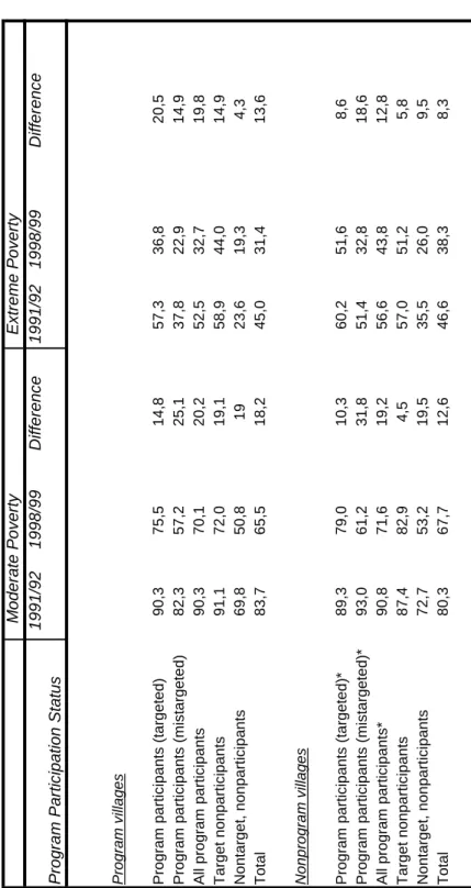
Following Khander’s carefully study, we now examine in detail the poverty e¤ects of microcredit intervention. In his analysis, the author distinguishes between moderately poor and extremely poor (as argued in Khander, 1998, he de…nes moderate poverty as house-hold consumption level below 5,270 taka/person/year and extreme poverty as 80% of that, 3,330 taka/person/year)27.
Table 1 contains data from Bangladesh context in Khander(2005). We can note, from this survey, that in program villages microcre-dit participants had relevant declines in poverty rates (in terms of moderate poverty). Concerning the voice "All program partic-ipants", we can see a decrease from a rate of about 90 percent in the …rst period to about 70 percent in the second round of data, approximately a 20 percentage point decline. But for el-igible households that did not participate in credit programmes (in the period 1991/92) the falling in terms of poverty rate was 19.2 percentage points, as nontarget nonparticipants (19 percent). At this point, the question is: did microcredit intervention play a role in this process? Pessimists may answer that the decline of average poverty incidence for program participants might have happened even without intervention. On the other hand, optimists think that the net impact of programmes have been substantial, involving also nonparticipants. In other words, they argue that the spillover e¤ect could explain the general improvement in areas with programs. Comparing the results for program areas to results for villages without intervention in 1991/1992, we can note a sim-ilar trend: poverty rates decreased by around 19 to 20 percentage points (only target nonparticipants had a poverty reduction of 4.5 percentage points).
In his conclusions, Khander argues that microcredit contributed to approximately one third to one half of these poverty contractions. Speci…cally, Khander asserts that lending 100 taka to a female leads to a growth in household consumption by around 8 taka annually. Moreover, he suggests that the impact of micro…nance intervention is stronger for extreme poverty than moderate poverty, and microcredit e¤ects are more relevant for women borrowing than for men borrowing.
4.4 The Roodman-Morduch revisitation.
The Roodman-Morduch approach to PK’s analysis a¢ rms, as Mor-duch (1998), that the baseline assumptions used in the study do not hold. Morduch (1999) does not …nd evidence of consumption impacts in the 1991/1992 data and criticizes the identifying as-sumptions of the PK’s framework. On the other hand, he suggests that microcredit decreases consumption volatility. In their replica-tion, Roodman and Morduch (2009) use the same methods to the same data as in PK. Applying two-stages least-squares (2SLS) re-gression, they contest the positive results obtained in the previous study. Concerning the PK …ndings, Roodman-Morduch achieve opposite (in sign) results. On the basis of speci…c tests , they argue that instrumentation strategy is failing. Reverse or omitted-variable causation drives the …nal outcomes, and the endogenous links between credit and consumption varies by subsample ( i.e., borrower sex). It can explain the di¤erences in terms of gender impact. But they do not conclude that microcredit does not a¤ect the lives of poor borrowers; rather, they suggest that the statistical setting is not due to the task.
Roodman and Morduch …ndings about Khander’s analysis reduce the con…dence that the key identifying assumptions for causal infer-ence e¤ectively hold in a similar context. In particular, they doubt that the Khander’s assertion concerning the relevant impact of mi-crocredit services in reducing extreme poverty could arise from a direct estimation. The critical point is that the introduction of the panel framework does not seem to overcome the problem of the lack of clearly exogenous variations in the use of microcredit. The distinction between moderately poor and extremely poor con-ducted by the author is based on estimated baseline poverty levels. Then he compares changes in consumption (about the two kinds of poor households) using regression coe¢ cients that would have sense only if all the households have similar net impacts.
All the three studies (Pitt-Khander 1998, Morduch 1998, Khander 2005) tend to reinforce the general positive idea about microcre-dit. According to PK (1998) and Khander (2005), microloans can reduce poverty, especially for women. In addition, Morduch (1998) suggests that small-size credits help households to attenuate con-sumption variability across the seasons. Roodman and Morduch (2009) do not contradict these considerations, but highlight the absence of decisive statistical evidence in support of these studies.
5.
Randomized approach
5.1 Randomization as potential solution of selection bias: analyti-cal foundations.
As discussed in section 3, selection bias represents a relevant prob-lem in order to obtain a clean estimation of the microcredit pro-gram impact.
The aim, in this particular context, is to gauge the net e¤ect of credit access on the revenue of a borrower. The causal impact, that is the term E(Yi1 Yi0=Ti = 1) , is not observable but as argued
in Du‡o et. al. (2007) is "logically well de…ned".
Randomized experiments allow to manage selection bias problems through a random assignment of the program to the treatment and comparison groups.
How does this methodology function in practice?
First, a sample of N individuals, or households, is selected from a population of interest28; second, the initial sample is randomly
divided into two distinct subgroups: treatment and comparison or control groups.
The target units are exposed to the "treatment" (i.e. they receive the loan), while the non-target units aren’t. Then researchers ob-serve the outcome Y, and compared the results for both di¤erent subgroups.
As argued in section 3, we can estimate the average program im-pact as follows:
=E(Y1
i =Ti = 1) E(Yi0=Ti = 0) (8)
The advantage in adopting this approach is that the two groups are expected to be identical before the microcredit program, be-cause of their random selection. The only di¤erence is due to the exposure of the treatment. This implies that the selection bias term E(Y0
i =Ti = 1) E(Yi0=Ti = 0) is equal to zero.The term in
question describes how both participant group and control group would have performed if nobody had had access to credit. More-over, if the outcomes of a subject are unrelated to the treatment of the other individuals29, we obtain
28It’s important to highlight that the population of interest can’t be randomly
drawn from the whole population, but could be selected on the basis of observable attributes (Du‡o et al. 2007).
E(Y1
i =Ti = 1) E(Yi0=Ti = 0) =E(Yi1 Yi0=Ti = 1) =E(Yi1 Yio)
(9)
If randomization has been completed with success, experimental approaches can provide a valuable instrument in order to overcome selection bias problems.
In the opposite case, we can meet with problems. For instance, the individuals that apply for loans successfully may have more business ability, organizational skills and entrepreneurial experi-ence than subjects that don’t apply for a microcredit program. Besides, the choice of the location from a micro…nance institution may be addressed to the villages with good life and economic con-ditions respect to other more disadvantaged sites.
Many estimation problems concern the cases of "non-random" at-trition (the less promising clients are the …rst to drop out of the program) and contamination (for instance, a new competitor starts his …nancial activity during the study period).
Generally, the bias of impact estimation is upward. But there are also particular forms of selection bias, such as contamination, which may lead to downward biases; performing a correct random-ization implying that E(Yi0=Ti = 1) =E(Yi0=Ti = 0):30
5.2 Randomization in microcredit impact evaluations: sample-size
and the power of experiments.
In general, two particular factors a¤ect the success of an exper-iment: statistical power and the role of spillovers (Armendàriz, Morduch, 2010).
Du‡o et al. (2007) suggest the basic principles of power calcu-lation31, starting from a simple regression frame. The estimate of the average impact is the OLS coe¢ cient of in the following regression:
Yi = + T + i (10)
Following Bloom’s (1995) approach, we assume that only a possible treatment exists, and that a speci…c proportion P of the sample receives the treatment in question. Since we suppose that each
30As much as discussed above depends on the properties of expectations of linear
operators (average impact).
As argued in Armendàriz, Morduch (2010, p. 296): "But the basic set-up does not permit us to say anything about the medians and very little about the distributional features of impacts. And we need to be careful in analyzing data on the impacts for
particular subgroups in a population."
unit was randomly sampled from an identical population, the ob-servations can be considered to beidentical independent distributed
(i.i.d.), with variance 2:
Clearly, the variance of the OLS estimator of , that is ^ , is determined by:
1
P(1 P)
2
N (11)
Now, we focus our attention on testing the hypothesis H0 , that is
the impact of the treatment is equal to zero against the alternative hypothesis, H1 , that it is not.
The signi…cance level related to a speci…c test describes the likeli-hood of rejecting the null hypothesis when it’s true.
Figure 1: Statistical Power
Figure 1 draws two distinct bell shaped curves: on the left there is the distribution of ^ under the null hypothesis of absence of impact H0 = 0, on the right the distribution of ^ if the true e¤ect
is e¤ectively :
In the …rst speci…cation, If ^ falls to the right of the critical value, for a determinate level of signi…cance, the hypothesis H0 = 0 will
be rejected; formally, it is true if
j ^ j> ta SE^ (12)
whereta hinges on the signi…cance level and it derives from a
stan-dard t-distribution.
In the second case, in order to evaluate the power of the test for a true impact size we take into account the part of the area under this curve which is to the right of the critical level ta. In
other words, it corresponds to the probability of rejecting the null hypothesis when it’s e¤ectively false.
The achievement of a power k implies the following condition:
>(t1 k+ta)SE ^ (13)32
Du‡o et al. (2007) consider the issue of power as the "minimum detectable e¤ect size" for a given statistical power (k), signi…cance level (a), sample size (N), and set of individuals that belong to the treatment group (P). It can be given by
MDE=(t1 k+ta) q 1 P(1 P) q 2 N (14) 33
where the termt1 krepresents the level of statistical power,tacaptures
the con…dence level,P includes the portion of sample that received the program, 2 is the variance of the impact and, …nally,N is the
total size of the sample.
From equation (14), we note a trade-o¤ between statistical power and sample size. In fact, when N increases, the minimum de-tectable e¤ect size decreases, and vice versa. Power calculation describes the linkage between impact size and sample size, with typical statistical con…dence levels (5 percent, 10 percent, 20 per-cent). But in general the e¤ect size is not known before starting with the intervention. Many di¤erent studies have developed po-tential solutions to overcome such problems: the …rst practical approach consists in making predictions on the basis of previous researches, the second concerns the introduction of a small pilot study.34
Cohen (1988), for instance, express the impact size in terms of standard deviations from the mean of the outcome; he suggests, in his analysis, that an impact of 0.2 standard deviation is negligible, 0.5 is intermediate, and 0.8 is relevant. Clearly, these values are indicative and have to be considered in each speci…c context. Equation (14) also provides useful advice concerning the division of the sample between treated and non-treated units. We assume, for example, that there is a single treatment, and the most relevant cost of the study is data collection. It follows that an equal distrib-ution between treatment and control group is an optimal allocation (in this case, the equation above is minimized at P=0.5).
But if program implementation is costly and the data are easily available for both the groups ( the data collection process isn’t
ex-32The term t
1 k is simply given by at-table.
33It refers to a single sided test. If we introduce a two-sided test, the termta will
be substituted by ta=2:
pensive), the optimal division will require a larger control group. Speci…cally, in order to obtain the optimal proportion of treated units, equation (14) must be minimized under the budget con-straint as follows: M in P (t1 k+ta) q 1 P(1 P) q 2 N (15) sub Ncc+N P ct B
where N is the total sample size, cc represents the unit cost per
comparison subject, and ct is the unit cost for treatment subject.
From (10), we obtain the optimal allocation rule:
P
1 P =
pcc
ct (16)
As argued in Du‡o et al. (2007), "the ratio of subjects in the treatment group to those in the comparison should be proportional
to the inverse of the square root of their costs."
The above setting can be applied to sample size calculations when there are multiple treatment.35
The level of randomization represents a crucial matter for the sam-ple size. Many experimental designs involve randomization over groups rather than single individuals. For example, PROGRESA36 program used the village as the unit of randomization, even if sin-gle individual data were available for statistical evaluation.
In similar contexts, we have to consider that the error term may not be independent across single individuals. If the program par-ticipants in a group have some attributes in common, information about single units will cause weak variations in the …nal result compared to the case of individual-level randomization. Since bor-rowers of the same group can be subject to common shocks, a correlation between outcomes is very likely, and leads to a wrong interpretation of the program impact.37
The key issue is to compare the proportion of the outcome vari-ance coming from the group impact and the proportion coming from individual impact: if the …rst value is higher, also the sample needs to be bigger, or, alternatively, the e¤ective size necessary for detection.
35See Bloom (1995).
36PROGRESA(Programa de Educaciòn, Salud y Alimentaciòn) is an anti-poverty
program implemented in Mexico in the late 1990s (for more information, see http://www.ifpri.org/dataset/mexico-evaluation-progresa)
One important di¢ culty encountered when we operate in the mi-cro…nance context is that some experimental designs only encour-age subjects to participate in a speci…c credit program (treatment) so that "eligible" people can accept or refuse the invitation. At the same time, people in the control group may take up the treatment even if they are not directly encouraged (Armendàriz, Morduch, 2010).
Ashraf, Karlan, and Yin (2006) encouraged a randomly selected group of people to sign up a new savings account. In this frame-work, the element of randomness was the invitation; this implies that the e¤ects of the program must be evaluated comparing in-vited and non-inin-vited subjects. Clearly, it follows that not all invited individuals accepted the proposal. Since the impact mea-sured at the invitation level is reduced, a bigger sample size is required.
Finally, a strati…cation (or block) of the sample can be introduced in order to improve estimate precision. Stratifying involves divid-ing the sample into subgroups that have similar values of particular observable characteristics. Then, the randomization is conducted for each single block (subgroup) separately.
While the randomization procedure ensures that treatment and comparison groups will be similar in terms of expectation, strati…-cation process is used in order to ensure that the assignment to a speci…c group (treatment or control group) is random in practice, along observable dimensions of the strati…cation.
A strati…ed design allows us to gauge the impact of the program for each subgroups separately using statistical methods. Since each block tends to be more homogeneous compared to the entire sam-ple, a little change in the outcome levels can be found out with the same sample size. The relevant consequence is that a smaller total sample is needed38.
5.3 Spillover e¤ects
Experimental designs can make externalities such that non treated individuals are a¤ected by the intervention. Moreover, there are spillovers also when an individual transfers from the treatment group to the comparison group, or vice-versa.
Following Du‡o et al. (2007), we consider a simple case in which a microcredit program is randomly attributed across a population of