Multivariate Poisson hidden Markov models for analysis of spatial counts

MULTIVARIATE POISSON HIDDEN MARKOV MODELS

FOR ANALYSIS OF SPATIAL COUNTS

A Thesis Submitted to the Faculty of Graduate Studies and Research in Partial Fulfillment of the Requirements for the Degree of

Doctor of Philosophy

in the Department of Mathematics and Statistics University of Saskatchewan, Saskatoon,

SK, Canada

by

Chandima Piyadharshani Karunanayake

PERMISSION TO USE

The author has agreed that the libraries of this University may provide the thesis freely available for inspection. Moreover, the author has agreed that permission for copying of the thesis in any manner, entirely or in part, for scholarly purposes may be granted by the Professor or Professors who supervised my thesis work or in their absence, by the Head of the Department of Mathematics and Statistics or the Dean of the College in which the thesis work was done. It is understood that any copying or publication or use of the thesis or parts thereof for finanancial gain shall not be allowed without my written permission. It is also understood that due recognition shall be given to the author and to the University of Saskatchewan in any scholarly use which may be made of any material in this thesis.

Requests for permission to copy or to make other use of any material in the thesis should be addressed to:

Head

Department of Mathematics and Statistics University of Saskatchewan

106, Wiggins Road Saskatoon, Saskatchewan Canada, S7N 5E6

ABSTRACT

Multivariate count data are found in a variety of fields. For modeling such data, one may consider the multivariate Poisson distribution. Overdispersion is a problem when modeling the data with the multivariate Poisson distribution. Therefore, in this thesis we propose a new multivariate Poisson hidden Markov model based on the extension of independent multivariate Poisson finite mixture models, as a solution to this problem. This model, which can take into account the spatial nature of weed counts, is applied to weed species counts in an agricultural field. The distribution of counts depends on the underlying sequence of states, which are unobserved or hidden. These hidden states represent the regions where weed counts are relatively homogeneous. Analysis of these data involves the estimation of the number of hidden states, Poisson means and covariances. Parameter estimation is done using a modified EM algorithm for maximum likelihood estimation.

We extend the univariate Markov-dependent Poisson finite mixture model to the multivariate Poisson case (bivariate and trivariate) to model counts of two or three species. Also, we contribute to the hidden Markov model research area by developing Splus/R codes for the analysis of the multivariate Poisson hidden Markov model. Splus/R codes are written for the estimation of multivariate Poisson hidden Markov model using the EM algorithm and the forward-backward procedure and the bootstrap estimation of standard errors. The estimated parameters are used to calculate the goodness of fit measures of the models.

Results suggest that the multivariate Poisson hidden Markov model, with five states and an independent covariance structure, gives a reasonable fit to this dataset. Since this model deals with overdispersion and spatial information, it will help to get an insight about weed distribution for herbicide applications. This model may lead researchers to find other factors such as soil moisture, fertilizer level, etc., to determine the states, which govern the distribution of the weed counts.

Keywords: Multivariate Poisson distribution, multivariate Poisson hidden Markov model, Weed species counts, EM algorithm.

ACKNOWLEDGEMENT

First I would like to acknowledge and express my sincere thanks and gratitude to my supervisor Dr. William H. Laverty for his availability, continual guidance, valuable suggestions and encouragement throughout the course of study.

Next, I would like to thank the members of my advisory committee, Prof. R. Srinivasan, Prof. C. E. Soteros, Prof. M.J. Miket and Prof. I.W. Kelly for their valuable suggestions and advice in many aspects of my thesis completion. I am also grateful for comments and suggestions from my external examiner, Prof. Peter MacDonald.

My special thanks to Dr. Dimitris Karlis, Athens University of Economics, Athens, Greece for his valuable advice and help me solve the problems I had with multivariate Poisson distributions.

I am very grateful for the funding provided by College of Graduate Studies and Research and Depaerment of Mathematics and Statistics. Without their support and resources, it is impossible to complete this thesis.

I would also like to thank Ms. Jessica Antonio of the Department of English, University of Saskatchewan for proof reading this thesis.

Finally, my heartfelt thanks go to my dear parents, and especially my husband, Sumith Priyashantha, who always wished and encouraged me to successfully complete my study program in Canada.

DEDICATION

This thesis is dedicated to my loving parents, Prof. Marcus Marcy Karunanayake and Mrs. Sumana Piyaseeli Karunanayake, and my dearest husband, Kahanda Rathmalapage Sumith Priyashantha, who always gave me encouragement for the success in my academic career.

TABLE OF CONTENTS

PERMISSION TO USE ...i

ABSTRACT ...ii

ACKNOWLEDGEMENT...iv

DEDICATION ...v

TABLE OF CONTENTS ...vi

LIST OF TABLES ...ix

LIST OF FIGURES...xi

LIST OF ACRONYMS...xiii

1 GENERAL INTRODUCTION 1.1 Introduction ...1

1.2 Literature review ...2

1.2.1Introduction to finite mixture models...2

1.2.2 History of hidden Markov models...3

1.2.3 Hidden Markov model and hidden Markov random field model ...5

1.3 Outline of the thesis...8

2 HIDDEN MARKOV MODELS ( HMM’s) AND HIDDEN MARKOV RANDOM FIELDS (HMRF’s) 2.1 Discrete time finite space Markov chain ...9

2.2 Examples of hidden Markov models...10

2.3 Definition of the hidden Markov model ...17

2.4 Definition of the hidden Markov random field model ...20

2.4.1 Markov random fields ...20

2.4.2 Hidden Markov random field (HMRF) model ...26

3 INFERENCE IN HIDDEN MARKOV MODELS 3.1 Introduction ...29

3.2 Solutions to three estimation problems ...30

3.2.1 Problem 1 and its solution ...30

3.2.2 Problem 2 and its solution ...35

3.2.3 Problem 3 and its solution ...37

4 HIDDEN MARKOV MODEL AND THEIR APPLICATIONS TO WEED COUNTS 4.1 Introduction ...43

4.2 Weed species composition ...44

4.2.1 Wild Oats...45

4.2.1.1 Effects on crop quality...45

4.2.2 Wild Buckwheat ...46

4.2.2.1 Effects on crop quality...47

4.2.3 Dandelion ...47

4.3 Problem of interest and proposed solution ...48

4.4 Goals of the thesis ...53

5 MULTIVARIATE POISSON DISTRIBUTION, MULTIVARIATE POISSON FINITE MIXTURE MODEL AND MULTIVARIATE POISSON HIDDEN MARKOV MODEL 5.1 The multivariate Poisson distribution: general description ...55

5.1.1 The fully- structured multivariate Poisson model ...59

5.1.2 The multivariate Poisson model with common covariance structure...63

5.1.3 The multivariate Poisson model with local independence ...65

5.1.4 The multivariate Poisson model with restricted covariance...66

5.2 Computation of multivariate Poisson probabilities ...68

5.2.1 The multivariate Poisson distribution with common covariance...70

5.2.2 The multivariate Poisson distribution with restricted covariance ...73

5.2.3 The Flat algorithm ...75

5.3 Multivariate Poisson Finite mixture models...78

5.3.1 Description of model-based clustering...79

5.3.2 Model-based cluster estimation...82

5.3.3 ML estimation with the EM algorithm...82

5.3.3.1 Properties of the EM algorithm ...84

5.3.4 Determining the number of components or states ...85

5.3.5 Estimation for the multivariate Poisson finite mixture models ...87

5.3.5.1 The EM algorithm ...87

5.4 Multivariate Poisson hidden Markov models...91

5.4.1 Notations and description of multivariate setting...91

5.4.2 Estimation for the multivatiate Poisson hidden Markov models...92

5.4.2.1 The EM algorithm ...93

5.4.2.2 The forward-backward algorithm...95

5.5 Bootstrap approach to standard error approximation ...98

5.6Splus/R code for multivariate Poisson hidden Markov model ...102

5.7 Loglinear analysis...102

6 RESULTS OF MULTIVARIATE POISSON FINITE MIXTURE MODELS AND MULTIVARIATE POISSON HIDDEN MARKOV MODELS 6.1 Introduction ...108

6.2 Exploratory data analysis ...108

6.4Data analysis...114

6.4.1 Results for the different multivariate Poisson finite mixture models...115

6.4.2 Results for the different multivariate Poisson hidden Markov models ...123

6.5 Comparison of different models...131

7 PROPERTIES OF THE MULTIVARIATE POISSON FINITE MIXTURE MODELS 7.1 Introduction ...138

7.2 The multivariate Poisson distribution...139

7.3 The properties of multivariate Poisson finite mixture models ....141

7.4 Multivariate Poisson-log Normal distribution...145

7.4.1 Definition and the properties ...145

7.5 Applications...147

7.5.1 The lens faults data ...147

7.5.2 The bacterial count data...152

7.5.3 Weed species data...156

8 COMPUTATIONAL EFFICIENCY OF THE MULTIVARIATE POISSON FINITE MIXTURE MODELS AND MULTIVARIATE POISSON HIDDEN MARKOV MODELS 8.1 Introduction ...161

8.2 Calculation of computer time ...161

8.3 Results of computational efficiency ...162

9 DISCUSSION AND CONCLUSION 9.1 General summary...168

9.2 Parameter estimation ...170

9.3 Comparison of different models...171

9.4 Model application to the different data sets...174

9.5 Real world applications ...174

9.6 Further research ...177

REFERENCES ...179

APPENDIX ...192

A. Splus/R code for Multivaraite Poisson Hidden Markov Model- Common Covariance Structure ...192

B. Splus/R code for Multivaraite Poisson Hidden Markov Model- Restricted and Independent Covariance Structure...200

LIST OF TABLES Table 6.1: Mean, variance and variance/mean ratio for the

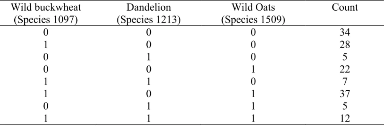
three species...110 Table 6.2: Univariate Poisson mixture models...110 Table 6.3: Correlation matrix of three species ...112 Table 6.4: The frequency of occurrence (present/ absent) of

Wild buckwheat, Dandelion and Wild Oats ...113 Table 6.5: The likelihood ratio (_G2_{) test for the different models of the}

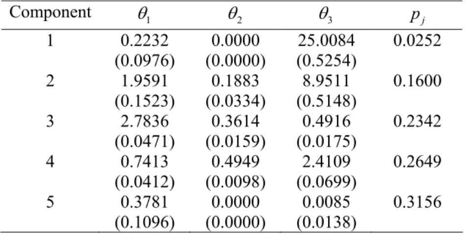
Wild buckwheat, Dandelion and Wild Oats counts...113 Table 6.6: Parameter estimates (bootstrap standard errors) of the five

components independence covariance model...118 Table 6.7: Parameter estimates (bootstrapped standard errors) of the five components common covariance model...120 Table 6.8: Parameter estimates (bootstrapped standard errors) of the four component restricted covariance model ...123 Table 6.9: Parameter estimates (bootstrapped standard errors) of the five states hidden Markov independence covariance model ...128 Table 6.10: Transition probability matrix of the hidden Markov

independence covariance model...128 Table 6.11: Parameter estimates (bootstrapped standard errors) of the five states hidden Markov common covariance model ...129 Table 6.12: Transition probability matrix of hidden Markov common

covariance model...129 Table 6.13: Parameter estimates (bootstrapped standard errors) of the four states hidden Markov restricted covariance model ...130 Table 6.14: Transition Probability matrix of the hidden Markov

restricted covariance model ...130 Table 7.1: Counts (x x₁, ₂) of surface and interior faults in 100 lenses...147 Table 7.2: Loglikelihood, AIC and BIC together with the number of

components for the common covariance multivariate

Poisson finite mixture model ...148 Table 7.3: Loglikelihood, AIC and BIC together with the number of

components for the local independence multivariate

Poisson finite mixture model ...149 Table 7.4: Loglikelihood, AIC and BIC together with the number of

components for the common covariance

multivariate Poisson hidden Markovmodel ...150 Table 7.5: Loglikelihood, AIC and BIC together with the number of

components for the local independence

multivariate Poisson hidden Markovmodel ...150 Table 7.6: Bacterial counts by 3 samplers in 50 sterile locations...153

Table 7.7: Loglikelihood and AIC together with the number of

components for the local independence multivariate Poisson

finite mixture model ...154 Table 7.8: Loglikelihood and AIC together with the number of

components for the local independence

multivariate Poisson hidden Markovmodel ...155 Table 8.1: Independent covariance structure –CPU time

(of the order of 1/100 second) ...163 Table 8.2: Common covariance structure –CPU time

(of the order of 1/100 second) ...164 Table 8.3: Restricted covariance structure –CPU time

LIST OF FIGURES

Figure 2.1: 1- coin model ...11

Figure 2.2: 2- coins model...12

Figure 2.3: 3- coins model...13

Figure 2.4: 2-biased coins model...15

Figure 2.5: The urn and ball model ...17

Figure 2.6: Two different neighbourhood structures and their corresponding cliques...22

Figure4.1: Wild Oats ...45

Figure 4.2: Wild Buckwheat...46

Figure 4.3: Dandelion...48

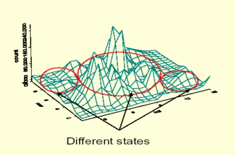
Figure 4.4: Distribution of weed counts in field #1...49

Figure 4.5: Data collection locations from field #1...50

Figure 4.6: Distribution of Weed Counts and Different States (clusters) in Field #1...50

Figure 4.7: Scanning method: Line Scan ...51

Figure 5.1: Flat algorithm (stage 1)...76

Figure 5.2: Calculating p(2, 2, 2) using the Flat algorithm ...76

Figure 5.3: Flat algorithm (stage 2)...77

Figure 5.4: Calculating (2, 2)p using the Flat algorithm...77

Figure 6.1: Histograms of species counts (a) Wild Buckwheat, (b) Dandelion and (c) Wild Oats ...109

Figure 6.2: Scatter plot matrix for three species...111

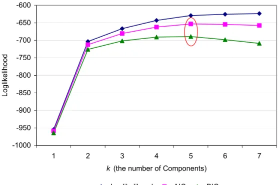
Figure 6.3: Loglikelihood, AIC and BIC against the number of components for the local independence multivariate Poisson finite mixture model...116

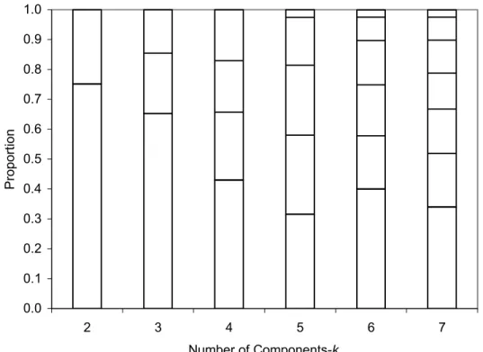
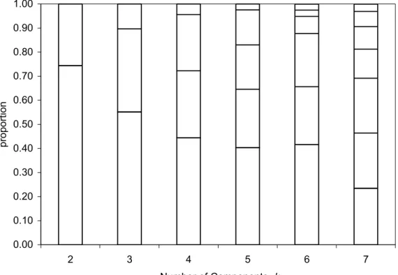
Figure 6.4: The mixing proportions for model solutions with k= 2 to 7 components for the local independence multivariate Poisson finite mixture model ...117

Figure 6.5: Loglikelihood, AIC and BIC against the number of components for the common covariance multivariate Poisson finite mixture model ...119

Figure 6.6: The mixing proportions for model solutions with k= 2 to 7 components for the common covariance multivariate Poisson finite mixture model ...120

Figure 6.7: Loglikelihood, AIC and BIC against the number of components for the restricted covariance multivariate Poisson finite mixture model ...121

Figure 6.8: The mixing proportions for model solutions with k= 2 to 7 components for the restricted covariance multivariate Poisson finite mixture model...122

Figure 6.9: Loglikelihood, AIC and BIC against the number of states for the local independent multivariate Poisson hidden Markovmodel ...125

Figure 6.10: Loglikelihood, AIC and BIC against the number of states for the common covariance multivariate Poisson hidden

Markovmodel ...126 Figure 6.11: Loglikelihood, AIC and BIC against the number of

states for the restricted covariance multivariate Poisson

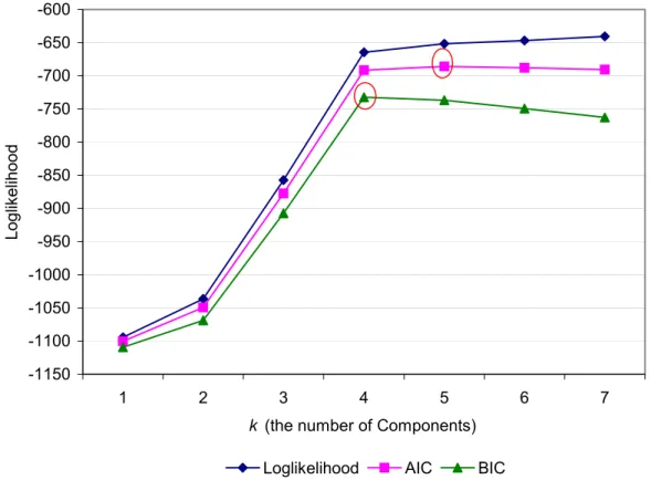
hidden Markovmodel...127 Figure 6.12: Loglikelihood against the number of components (k)

for the multivariate Poisson finite mixture models ...131 Figure 6.13: Loglikelihood against the number of components (k)

for the multivariate Poisson hidden Markov models...132 Figure 6.14: Contour plot of clusters for the (a) independent, (b) common

and (c) restricted covariance multivariate Poisson finite

mixture models ...136 Figure 6.15: Contour plot of clusters for the (a) independent, (b) common and (c) restricted covariance multivariate Poisson hidden

Markovmodels...137 Figure 8.1: Sample Size vs CPU time for different models of the

Independent covariance structure ...165 Figure 8.2: Sample Size vs CPU time for different models of the common covariance structure...166 Figure 8.3: Sample Size vs CPU time for different models of the restricted covariance structure...167

LIST OF ACRONYMS

AIC Akaike Information Criterion BIC Bayseian Information Criterion

EM Expectation- Maximization

GIS Geographic Information System

GLM Generalized Linear Model

HMM Hidden Markov Model

HMRF Hidden Markov Random Field

LRT Likelihood Ratio Test

MFM Multivariate Finite Mixture

ML Maxiumum Likelihood

MRF Markov Random Field

CHAPTER 1

GENERAL INTRODUCTION

1.1Introduction

The analysis of multivariate count data (e.g. weed counts for different species in a field) that are overdispersed relative to the Poisson distribution (i.e. variance > mean) has recently received considerable attention (Karlis and Meligkotsidou, 2006; Chib and Winkelmann, 2001). Such data might arise in an agricultural field study where overdispersion is caused by the individual variability of experimental units, soil types or fertilizer levels. Therefore, these data (e.g. weed counts) are not homogenous within the field. The Poisson mixture model is a flexible alternative model which can represent the inhomogeneous population. Finite Poisson mixtures are very popular for clustering since they lead to a simple and natural interpretation, as models describing a population consisting of a finite number of subpopulations.

These types of count data can be modelled using model-based clustering methods, such as multivariate Poisson finite mixture models (or independent finite mixture models) and multivariate Poisson hidden Markov models (or Markov-dependent finite mixture models). It is assumed that the counts follow independent Poisson distributions

conditional on rates, which are generated from an independent mixing distribution for finite mixture models. The counts for multivariate Poisson hidden Markov models are assumed to follow independent Poisson distributions, conditional on rates with Markov dependence. Finite mixture models can be particularly attractive because they provide plausible explanations for variation in the data (Leroux and Puterman, 1992).

1.2Literature review

1.2.1 Introduction to finite mixture models

The main question here is determining the structure of clustered data when no information other than the observed values is available. Finite mixture models have been proposed for quite sometime as a basis for studying the clustered data (Symons, 1981; McLachan, 1982; McLachlan et al., 1988). In this approach, the data are viewed as coming from a mixture of probability distributions, each representing a different cluster. Recently, finite mixture model analysis have been used in several practical applications: character recognition (Murtagh and Raftery, 1984); tissue segmentation (Banfield and Raftery, 1993); minefield and seismic fault detection (Dasgupta and Raftery, 1998); identification of textile flaws from images (Campbell et al., 1997); and classification of astronomical data (Celeux et al., 1995). Most of these examples are based on Gaussian finite mixture models. There are some examples of Poisson finite mixtures. Leroux and Puterman (1992) describe a univariate Poisson finite mixture model for fetal movement data. The clustering of cases of a rare disease (sudden infant death syndrome), on the basis of the number of cases observed for various counties in

North Carolina, is modelled by Symons et al. (1983) using a mixture of two Poisson distributions, which describe the two groups of high and low risk counties. Very recently, a multivariate Poisson finite mixture model was used for a marketing application (Brijs et al., 2004). Brijs describes a multivariate Poisson finite mixture model for clustering supermarket shoppers based on their purchase frequency in a set of product categories.

In this thesis, the multivariate Poisson finite mixture model is applied for the first time to weed species counts in an agricultural field. Also, we developed a multivariate Poisson hidden Markov model and applied it to analyze the weed species data. The goodness of fit measure of the model is also evaluated (Chapter 7). Details about multivariate Poisson finite mixture models and multivariate Poisson hidden Markov models are given in Chapter 5. The history of hidden Markov models is presented in the next section.

1.2.2 History of hidden Markov models

Hidden Markov Models (HMMs) are statistical models that are widely used in many areas of probabilistic modeling. These models have received increasing attention (Rabiner and Juang, 1986, 1991 and Rabiner, 1989), partially because of their mathematical properties (they are rich in mathematical structure), but mostly because of their applications to many important areas in scientific research.

Hidden Markov Models have been found to be extremely useful for modeling stock market behavior. For example, the quarterly change in the exchange rate of the dollar can be modelled as an HMM with two states, which are unobservable and correspond to the up and down changes in exchange rate (Engel and Hamilton, 1990). HMM is also used in the area of speech recognition. Juang and Rabiner (1991) and Rabiner (1989) described how one could design a distinct hidden Markov model for each word in one’s vocabulary, in order to envision the physical meaning of the model states as distinct sounds (e.g. Phonemes, syllables). A hidden Markov model for ecology was introduced by Baum and Eagon (1967). Later, they introduced a procedure for the maximum likelihood estimation of the HMM parameters for the general case where the observed sequence is a sequence of random variables with log-concave densities (Baum et al., 1970). In molecular biology, hidden Markov models are used to allow for unknown rates of evolution at different sites in a molecular sequence (Felsenstein and Churchill, 1996). Similarly, in climatology, the occurrence or nonoccurrence of rainfall at different sites can be modelled as an HMM where the climate states are unobservable, accounting for different distributions of rainfall over the sites (Zucchini et al., 1991).

The distinction between non-hidden Markov models and hidden Markov models is based on whether the output of the model is the actual state sequence of the Markov model, or if the output is an observation sequence generated from the state sequence. For hidden Markov models, the output is not the state sequence, but observations that are probabilistic function of the states. Thus in hidden Markov models, it extends the

concept of Markov models to include the case where the observation is a probabilistic function of the states.

The concept of hidden Markov Model has been the object of considerable study since the basic theory of hidden Markov models was initially introduced and studied during the late 1960’s and early 1970’s by Baum and his colleagues (Baum et al., 1966, 1967 and 1970). The primary concern in the hidden Markov modeling technique is the estimation of the model parameters from the observed sequences. One method of estimating the parameters of the hidden Markov models is to use the well-known Baum-Welch re-estimation method (Baum and Petrie, 1966). Baum and Eagon first proposed the algorithm in 1967 for the estimation problem of hidden Markov models with discrete observation densities. Baum and others (1970) later extended this algorithm to continuous density hidden Markov models with some limitations.

1.2.3 Hidden Markov model and hidden Markov random field model

Hidden Markov models are well known models in modeling the unknown state sequence given the observation sequence. As mentioned in the previous section, this has been successfully applied in the fields of speech recognition, biological modeling (protein sequences and DNA sequences) and many other fields. The hidden Markov models presented in section 1.2.2 are one-dimensional models, and they cannot take spatial dependencies into account. To overcome this drawback, Markov random fields and hidden Markov random fields (HMRF) can be used in more than one dimension when considering the spatial dependencies. For example, when the state space or

locations have two coordinates, that state space can be considered as a two-dimensional nearest-neighbor Markov random field. These Markov random fields have been extensively applied in the field of image processing (Fjφrtoft et al., 2003; Pieczynski et al., 2002; Zhang et al., 2001; Fjφrtoft et al., 2001; Aas et al., 1999).

In each case, there is a set of quantities, x, representing some unobservable phenomenon, and a supplementary set of observables, y. In general, y is a distorted version of x. For example, in the context of speech recognition, x represents a time sequence of configurations of an individual’s vocal tract; the y represents the corresponding time sequence of projected sounds. Here, the Markovian assumption would be that the elements of x come form a realization of a Markov chain. In the context of image analysis, x represents the true scene, in terms of the true pixellated colouring, and y denotes the corresponding observed image. Here, the Markovian assumption would be that the elements of x would be assumed to come from a Markov random field. The elements of x are indexed by a set, ,S of sites, usually representing time-points or discrete points in space (Archer & Titterington, 2002).

There is a very close relationship between Markov random fields and Markov chains. Estimation of Markov random field prior parameters can be done using Markov chain Monte Carlo Maximum likelihood estimation (Descombes et al., 1999). It is also demonstrated that a 2-D Markov random field can be easily transformed into a one-dimensional Markov chain (Fjφrtoft et al., 2003). Fjφrtoft (2003) explains that in image analysis, hidden Markov random field (HMRF) models are often used to impose spatial

regularity constraints on the underlying classes of an observed image, which allow Bayesian optimization of the classification. However, the computing time is often prohibitive with this approach. A substantially quicker alternative is to use a hidden Markov model (HMM), which can be adapted to two-dimensional analysis through different types of scanning methods (e.g. Line Scan, Hilbert-Peano scan etc.). Markov random field models can only be used for small neighbourhoods in the image, due to the computational complexity and the modeling problems posed by large neighbourhoods (Aas et al., 1999). Leroux and Puterman (1992) used maximum–penalized likelihood estimation to estimate the independent and the Markov-dependent mixture model parameters. In their analysis, they focus on the use of Poisson mixture models assuming independent observations and Markov-dependent models (or hidden Markov Models) for a set of univariate fetal movement counts. Extending this idea, for a set of multivariate Poisson counts, a novel multivariate Poisson hidden Markov model (Markov-dependent multivariate Poisson finite mixture model) is introduced. These counts can be considered as a stochastic process, generated by a Markov chain whose state sequence cannot be observed directly but which can be indirectly estimated through observations. Zhang et al. (2001) described that the finite mixture model is a degenerate version of the hidden Markov random field model. Fjφrtoft (2003) explained that the classification accuracy of hidden Markov random fields and hidden Markov models were not differing very much. Hidden Markov models are much faster than the ones based on the Markov random fields (Fjφrtoft et al., 2003). The advantage of hidden Markov models compared to the Markov random field models is the ability to combine

the simplicity of local modeling with the strength of global dependence by considering one-dimensional neighbourhoods (Aas et al., 1999).

1.3Outline of the thesis

Chapter 2 gives a review of the Markov process, and then gives examples of hidden Markov models to clarify and present the general definition of the HMM and the HMRF. Chapter 3 is about the prediction, the state identification and the estimation problem, the solution of the HMM for a univariate case. The question of interest in this thesis is presented in Chapter 4. Details about calculating multivariate Poisson probabilities, multivariate Poisson finite mixture models and multivariate Poisson hidden Markov models are discussed in Chapter 5. We extended the univariate Markov-dependent Poisson mixture model to a multivariate Poisson case (bivariate and trivariate). Also, we contributed to the hidden Markov model research area by developing Splus/R codes for the analysis of the multivariate Poisson hidden Markov Model. Splus/R codes are written to estimate the multivariate Poisson hidden Markov Model using the EM algorithm and the forward-backward procedure and the bootstrap estimation of standard errors. Results are presented in Chapter 6. The properties of the finite mixture models and several applications are presented in Chapter 7. The Computational efficiency of the models is discussed in Chapter 8. The discussion, conclusion and the areas of further research are presented in Chapter 9.

CHAPTER 2

HIDDEN MARKOV MODELS ( HMM’s) AND HIDDEN MARKOV RANDOM FIELDS(HMRF’s)

2.1 Discrete time finite state Markov chain

Let { ,S t_t =0,1, 2,....} be a sequence of integer valued random variables that can assume only an integer value {1, 2,...., }.K Then { ,S t_t =0,1, 2,....} is a K state Markov chain if the probability that S_t equals some particular value (j), given the past, depends only on the most recent value of S_t−1. In other words,

1 2 1

[ _t | _t , _t ,....] [ _t | _t ] _ij P S = j S₋ =i S₋ =m =P S = j S₋ = =i P ,

where

{ }

P_{ij i,j=1,2,...,K} are the one-step transition probabilities (Srinivasan and Mehata, 1978; Ross, 1996). The transition probability, P_ij, is the probability of transitioning

from state i to state j in one time step. Note that 1 1, 0. K ij ij j P P = = ≥

∑

Here, the output of the process is the set of states at each instant of time, where each state corresponds to an observable event. The above stochastic process is called an observable discrete time finite state Markov model.

2.2 Examples of hidden Markov models

In this section, we will give examples where the idea of the hidden Markov model (Rabiner, 1989; Elliott et al., 1995) is discussed and presented, in order to understand the concept of the HMM.

Examples:

1. A person is repeatedly rolling one of two dice picked at random, one of which is biased (unbalanced) and the other is unbiased (balanced). An observer records the results. If the dice are indistinguishable to the observer, then the two ‘states’ (i.e. biased dice or unbiased dice) in this model are hidden.

2. Consider an example of coin tossing. One person (person A) is in a room with a barrier (e.g., a curtain) through which he cannot see what is happening on the other side, where another person (person B) is performing a coin tossing experiment. Person B will tell person A the results of each coin flip. Person A only observes the results of the coin tosses, and he does not know anything about which coin gives the results. So the tossing experiment is hidden, providing a sequence of observations consisting of a series of heads and tails (T stands for tails and H stands for heads).

For example : Y1 Y2 …YT H T … H.

Given the coin tossing experiment, the question of interest is how to build hidden Markov models that will explain the observation sequence. For example 2, we can consider several models: 1-coin model, 2-coins model and 3-coins model.

1-coin model:

Here, there are two states in the model, but each state is uniquely associated with either head (state 1) or tail (state 2); hence, this model is not hidden because the observation sequence uniquely defines the state.

Y = H H T T H T H H T T H…… S = 1 1 2 2 1 2 1 1 2 2 1…..

Figure 2.1: 1- coin model

2-coins model:

There are two states in this model corresponding to a different, biased, coin being tossed; neither state is uniquely associated with either head or tail. Each state is characterized by a probability distribution of heads and tails, and the state transition matrix characterizes the transitions between the states. This matrix can be selected by a set of independent coin tosses or some other probabilistic event. The observable output sequences of 2-coins model are independent of the state transitions. This model is

1-P[H]

P[H] P[T]

P[H]

1 2

P[H]- The probability of observing a head P[T]- The probability of observing a tail 1-P[H]- The probability of leaving state 1

hidden because we do not know exactly which coin (state) led to the head or tail of each observation.

P11- The probability of staying in state 1 P22- The probability of staying in state 2 1-P11- The probability of leaving state 1 1-P22- The probability of leaving state 2

Y = H H T T H T H H T T H…… S = 2 1 1 2 2 2 1 2 2 1 2…..

(1) P[H]=P1 (2) P(H)=P2 P[T]=1-P1 P[T]=1-P2 ,

where (1) is the probability distribution of heads and tails in state 1 and (2) is the probability distribution of heads and tails in state 2.

Figure 2.2: 2- coins model

3-coins model:

The third form of the HMM for explaining the observed sequence of coin tossing outcomes is given in Figure 2.3. This model corresponds to the example using three biased coins, and choosing from among the three based on some probabilistic event.

1-P11

P11 P22

1-P22

P11- The probability of staying in state 1 P22- The probability of staying in state 2 P33- The probability of staying in state 3

P12- The probability of leaving state 1 and reaching state 2 P21- The probability of leaving state 2 and reaching state 1 P13- The probability of leaving state1 and reaching state 3 P31- The probability of leaving state 3 and reaching state 1 P32- The probability of leaving state 3 and reaching state 2 P23- The probability of leaving state 2 and reaching state 3

Y = H H T T H T H H T T H…… S = 3 1 2 3 3 1 1 2 3 1 3…..

(1) P[H]=P1 (2) P[H]=P2 (3) P[H]=P3 P[T]=1-P1 P[T]=1-P2 P[T]=1-P3,

where (1) is the probability distribution of heads and tails in state 1, (2) is the probability distribution of heads and tails in state 2 and (3) is the probability distribution of heads and tails in state 3.

Figure 2.3: 3- coins model

3 P32 P11 P22 P21 1 2 P12 P33 P13 P31 P23

Sample calculation of hidden Markov model (HMM)

A hidden Markov model is defined by specifying following five things: Q= the set of states ={1, 2,..., }.k

V = the output observations ={ , ,..., },v v_{1 2} v_m where m is finite number.

=

) (i

π Probability of being in state i at time t=0 (i.e. in initial states). A = transition probabilities = { },P_ij where

ij

P =P[entering state j at time t+1|in state i at time t] = P[S_t+1= j S| _t =i].

Note that the probability of going from state i to state j does not depend on the previous states at earlier times. This is called as Markov property.

B= output probabilities =

{

b_j(m)

}

,

where

{

b_j(m)

}

=P[producing v_m at time t| in statej at time t].

The above definition of a HMM applies to the special case where one has discrete states and discrete observations (Elliott et al., 1995).

Consider the case with the 2- biased coins model in Figure 2.4. Here, two biased coins were flipped, and an observer was seeing the results of the coin flip but not which coin was flipped. The states of the HMM are 1 and 2 (two coins), the output observation is {H, T}, and transition and output probabilities are as labeled. Let the initial state probabilities are π(1)=1 and π(2)=0. This model has two states corresponding to two different coins. In state 1, the coin is biased strongly towards heads and in state 2 ; the coin is biased strongly towards tails. The state transition probabilities are 0.8, 0.6, 0.2, and 0.4.

(1) P [H]=2/3 (2) P [H]=1/6

P [T]=1/3 P [T]=5/6

Figure 2.4: 2-biased coins model

0.8 0.8 0.2 0.6 0.4 0.8 1 Æ 1 Æ 1 Æ 2 Æ 2 Æ 1 Æ 1

H H T T T T H The probabilities for the following events can be calculated as follows:

1. The probability of the above state transition sequence:

P[1112211]= π(1)P11P11P12P22P21P11=1 0.8 0.8 0.2 0.6 0.4 0.8 0.025.× × × × × × =

2. The probabilities of the above output sequence given the above transition sequence:

P[(HHTTTTH)|( 1112211)]=2 2 1 5 5 1 2

3 3 3 6 6 3 3× × × × × × =0.023.

3. The probability of the above output sequence and the above transition sequence: P[(HHTTTTH)∩( 1112211)]=_{0.025 0.023 5.7 10× = ×} −4_. 0.8 0.6 0.2 1 0.4 2

In this case, the results of the coin flips and which coins are being flipped are known. In general, which coins are being flipped is unknown. That is, the underlying model is known and the output sequence is observed, while the state sequence is “hidden.” In this case, the 2-biased-coins model is a hidden Markov model.

In the above examples, the outcomes of the tossed coins are T or H and only two observations are possible. More general situation is explained below: considering a set of N urns and each urn consisting of several colored balls (M).

The urn and ball model

Consider the situation where there are N urns in a room, and within each urn there are M distinct colours of balls (Figure 2.5). The physical process for obtaining observations is as follows. A person is in a room, and using some random process, he (or she) chooses an initial urn. From this urn, a ball is chosen at random, and its color is recorded as the observation. The ball is then replaced in the urn from which it was selected. A new urn is then selected according to the random selection process associated with the current urn, and the ball selection process is repeated. This entire process generates a finite observation sequence of colours, which can be considered as the observational output of the HMM. Here, each state corresponds to a specific urn and the ball colour probability is defined for each state. The choice of urns is dictated by the state transition matrix of the HMM.

…

Urn 1 Urn 2 Urn N

P[Red]=b₁(1) P[Red]= b₂(1) P[Red]= (1)b_N P[Blue]=b₁(2) P[Blue]= b₂(2) P[Blue]=b_N(2) P[Green]= b₁(3) P[Green]= b₂(3) P[Green]=b_N(3) …

P[Orange]= b M₁( ) P[Orange]= b M₂( ) P[Orange]=b M_N( ) The observation sequence is

Y= {Green, Green, Red, Yellow, Blue, …, Orange, Blue}

Figure 2.5: The Urn and Ball Model

2.3 Definition of the hidden Markov model

A hidden Markov Model is a doubly stochastic process, with an underlying stochastic process that is not observable (hidden), and can only be observed through another set of stochastic processes that produced the sequence of observations.

Simply stated, a hidden Markov model is a finite set of states, each of them being associated with a probability distribution, and the transition between the states being covered by the transition probability. In particular, the observation can be generated according to the associated probability distribution so it is only the outcome that is

observable, not the states; therefore, the states are “hidden” to the observer, hence the name “Hidden Markov Model” (Rabiner, 1989; Elliott et al., 1995).

To define the hidden Markov model completely we need to define the elements of the HMM:

1. The length of the observation sequence, T. So the states sequence can be written as {S₁,S₂,...,S_T}and the observation sequence would be {Y₁,Y₂,...,Y_T}.

2. The number of states in the model, K. In the 2-coins model example, the states correspond to the choice of coins (i.e. two possible states). The state at time t is denoted as S_t throughout the thesis. In the Urn model, the number of states corresponds to the number of urns.

3. The number of distinct observation symbols per state, M. For the coin-tossing example, the observation symbols are simply the “H” and the “T”. Considering the more general Urn model, the numbers of distinct observation symbols are

M distinct colours.

4. A set of state transition probabilities A={ },P_ij

1

[ | ],

ij t t

P =P S₊ = j S =i 1≤i,j≤ K,

where S_t denotes the state at time t and P_ij denotes the transition probability which must satisfy the constraints

0 ij P ≥ , for all 1≤i,j≤K

∑

= = K j ij P 1 , 1 for all 1≤i≤K.

5. The probability distribution of the observation symbol in state j: B =

{

b_j(n)

}

( ) [

j n

b n =P v at time t |S_t = j], 1≤ j≤K, 1≤n≤ M , where v_n denotes the nth observation symbol in a given state j.

) (n

b_j should also satisfy the stochastic constraints 0 ) (n ≥ b_j , 1≤ j≤ K, 1≤n≤M and

∑

= = M n j n b 1 1 ) ( , 1≤ j≤K.

6. The above probability distribution is the case when the observations are discrete. The initial state distribution π =

{ }

π_i , where

1

[ ]

i P S i

π = = , 1≤ j≤K.

From above definitions, it is clear that a complete specification of an HMM involves three model parameters ( ,K M T, ) and three sets of probability parameters( , , )A Bπ . Therefore, for convenience, we can use the compact notation λ =(A,B,π) to denote the complete set of parameters of the model throughout the thesis.

Before we go further, there are some assumptions that are made in the theory of hidden Markov models for mathematical and computational tractability. First, it is assumed that the next state is dependent only on the current state, which is called the Markov assumption. That is,

1 1 1 0 0 1

[ _t | _{t t}, _{t t} ,..., ] [ _t | _{t t}] P S₊ = j S =i S₋ =i₋ S =i =P S₊ = j S =i .

Second, there is the homogeneity assumption (i.e. state transition probabilities are independent of the actual time at which the transition takes place)

1 1 1 2 1 2

[ _t | _t ] [ _t | _t ].

P S ₊ = j S = =i P S ₊ = j S =i

Third, the statistical independence of observations, i.e. suppose we have a sequence of observations Y={ , ,..., },Y Y_{1 2} Y_T and the sequence of states {S₁,S₂,...,S_T} then the probability distribution of generating the current observation depends only on the current state. That is,

1 1 1 [ | ,..., _{T T}; ] T [ _{t t}| _{t t}; ] t P S i S i λ P Y y S i λ = = = = =

∏

= = Y y ,

and these assumptions are used to solve the problems associated with hidden Markov models.

2.4 Definition of the hidden Markov random field model

In this section, the Markov random field model is introduced, followed by the definition of the hidden Markov random model (Kunsch, 1995; Elliott et al., 1995 and 1996; Fishman, 1996).

2.4.1 Markov random fields

A random field is a stochastic process defined on a two-dimensional set, that is, a region of the plane, or a set of even higher dimension. The two-dimensional case will be the

focus of this section. Random fields, which possess a Markov property, are called Markov random fields (Elliott et al., 1995 and 1996).

Let us generalize this idea in a two-dimensional setting. Let Zbe the set of integers, and let _S⊂Z2_{be a finite rectangular two-dimensional lattice of integer points. Typically, it}

will take S={0,1,...,n−1}×{0,1,...,m−1}, for some n and m. S is a two-dimensional lattice containing n×m points. The points in S are often called sites. To define a Markov structure on the set S, we define what is meant by two points being neighbours. Different definitions may suit different purposes, or applications. However, the following two general conditions should include in the definition.

(i) A site must be a neighbour of itself.

(ii) If t is neighbour of s, then s is a neighbour of t.

The second condition is a symmetry requirement. It can be written s~ if the sites t S

∈

t

s, are neighbours. Two common neighbourhood structures are given in Figure 2.6. If s is a site, the neighbourhood Ν_sof s can be defined as the set of all its neighbours; {Ν_s = ∈t S: ~ }.t s Hence, Figure 2.6 illustrates the neighbourhood of the middle site, for two different structures. In these structures, special care must be taken at the edge of the lattice S, since sites located there have smaller neighbourhoods. One way of defining the neighbourhood structure is “wrapping around” the lattice and define sites at the other end of the lattice as neighbours.

Concept of clique:

Cliques are particular subsets of the sites in S, defined in the following way: (i) Any single site s is a clique.

(ii) Any subset C⊂Sof more than one site is a clique if all pairs of sites in Care neighbours.

Hence, what the cliques look like depends on the neighbourhood system. Figure 2.6 shows what cliques there are for the two neighbourhood systems displayed therein. Note that these schematic cliques should be moved around over the lattice to find out all the subsets of sites that fit with the given pattern.

Figure 2.6: Two different neighbourhood structures and their corresponding cliques eight closest points are

neighbours (top), corresponding cliques (bottom)

four closest points are neighbours (top), corresponding cliques (bottom).

Now consider a random field { ( ) :X s s S∈ } defined on S, that is, a collection X(s)of random variables indexed by sites in S. These random variables are assumed to take their values in a finite set χ, the state space. Some examples of χ are χ ={−1,+1} and

}. ,..., 2 , 1 { r =

χ The set _χS_{is the set of elements of the form x={ ( ) :x s s S∈ }with}

χ s)∈

(

x for each s. An element of _χS_{will often called as a configuration (of the random}

field). Also often we can simply write this as X for { ( ) :X s s S∈ } and think of Xas a random variable with values in _χS_{, the set of configurations. Letting |S| denote the}

number of elements of S and similarly for χ, the number of elements of the configuration space _χS_{is |χ|}|S| _{and it is hence often extremely large. For example, if}

} 1 , 1 {− + =

χ and S is a lattice of size 128 128,× its size is ₂1282_{. If A is a subset of S,} write ( )X A for { ( ) :X s s A∈ }, that is the collection of random variables on A, and similarly for a particular configuration x={ ( ) :x s s S∈ }. The symbol \ denotes set-difference; for example, S\{s}is the set of sites in S except s, and write this difference as S\s. Now the random field { ( ) :X s s S∈ }is a Markov random field (MRF) on

S(with respect to the given neighbourhood structure) if

[ ( ) ( ) | ( \ ) ( \ )] [ ( ) ( ) | ( ) ( )]

P X s =x s X S s =x S s =P X s =x s X Ν_s =x Ν_s for all sites s∈S and all configurations _x∈χS. _{In other words, the distribution of ( )X s , given all other} sites, depends at the realized values in its neighbourhood only. These conditional distributions are often called the local specification of the MRF. Two examples are presented to get an idea of different MRF:

The Ising model

Assuming }χ ={−1,+1 and the neighbourhood structure to the left in Figure 2.6, an often used local specification is

exp( ( ) ( )) [ ( ) ( ) | ( ) ( )] exp( ( )) exp( ( )) x x P X x X x x x β β β ∈ ∈ ∈ = = = − +

∑

∑

s

∑

s s t Ν s s t Ν t Ν s t s s Ν Ν t t

for some real β; note that the denominator does not depend on x( )s and is only a normalizing factor to make the right hand side a proper distribution, summing to unity. This model is called the Ising model (McCoy et al., 1973; Binder, 1979; Binder et al., 1992), after German physicist Ising who invented it with the original purpose of using it as an idealized model of a ferromagnetic material. The sum in the exponent is positive if

( )

x s has the same sign as the most of its neighbours. Hence, if β>0 the sites interact such that configurations x with many neighbours of the same sign will have large probabilities. On the contrary, if β<0, configurations with many neighbours having opposite signs will have large probabilities.

The Potts model

If there is no particular assumption on χ, except it being finite, and any of the neighbourhood systems of Figure 2.6, or some other one, a possible local specification is exp( #{ : ( ) ( )}) [ ( ) ( ) | ( ) ( )] exp( #{ : ( ) }) i x x P X x X x x i β β ∈ ∈ ≠ = = = ∈ ≠

∑

s s s s χ t N t s s s Ν Ν t N t

for some real β. Again, the denominator does not depend on ( )x s and is only a normalizing factor. This model is called the Potts model (Binder, 1979; Wu, 1982; Binder et al., 1992). Note that, #{t N∈ _s: ( )x t ≠x( )}s is the number of neighbours of s that have values different from ( )x s . Hence, if β>0 this model gives large probabilities to configurations x in which there are many neighbours with different values. If β<0, the model works the opposite way, that is, configurations with many neighbours with equal values have large probabilities.

So far the local specification of a MRF is discussed, and it is also interesting to find out a corresponding distribution on _χS_{, that is, in the probabilities of various configurations}

x. This distribution can be denoted by π; hence,

( )x P X[ x] P X[ ( ) x( ), ]

π = = = s = s ∀ ∈s S

for any configuration _x∈χS_{. Now assume for each clique C there is a function}

: V χS →

C R. That is, VC maps a configuration x into a real number. Moreover, VC

must not depend on sites other than those in C. This can be written as ( ) ( ( )).

V x_C =V X_C C A probability mass function, or distribution, πon the configuration space _χS _{of the form}

1 ( )x Z exp V x( ) π ₌ −     

∑

C C 

is called a Gibbs distribution. Here the sum runs over all cliques C. The energy function is defined as ( )U x =

∑

V x_C( )

C

which is a sum of clique potentials V x_C( ) over all

exp x Z V ∈   = _{ }  

∑

∑

S _C C χ

and is generally infeasible to compute as the outer sum runs over a very large set. The importance of Gibbs distributions is made clear from the following facts:

(i) Any random field with a distribution π which is a Gibbs distribution is a Markov random field with respect to the neighbourhood system governing the cliques.

(ii) Any random field which is Markov with respect to a give neighbourhood system has a distribution π, which is a Gibbs distribution generated by the corresponding cliques.

Hence, according to the Hammersley-Clifford theorem (Fishman, 1996), an MRF can equivalently be characterized by a Gibbs distribution. For more details on the MRF and the Gibbs distribution, see Geman and Geman (1984).

2.4.2 Hidden Markov random field (HMRF) model

The concept of a hidden Markov random field model (Elliott et al., 1995 and 1996) is derived from the hidden Markov model, which is defined as stochastic processes generated by a Markov chain whose state sequence cannot be observed directly, only through a sequence of observations. Each observation is assumed to be a stochastic function of the state sequence. The underlying Markov chain changes its state according to a × transition probability matrix, where is the number of states.

Since original HMMs were designed as one-dimensional Markov chains with first-order neighborhood systems, it cannot directly be used in two-dimensional problems such as image segmentation. A special case of an HMM, in which the underlying stochastic process is an MRF instead of a Markov chain, is referred to as a hidden Markov random field model (Zhang et al., 2001). Mathematically, an HMRF model is characterized by the following:

• Hidden Markov Random Field (HMRF)

The random field X={X(s):s∈S} is an underlying HMRF assuming values in a finite state space L=(1,...., ) with probability distribution π. The state of X is unobservable.

• Observable Random Field }

: ) (

{ s s S

Y= Y ∈ is a random field with a finite state space D=(1,...,d). Given any particular configuration x∈χ, every Y( )s follows a known conditional probability distribution ( ( ) | ( ))p y s x s of the same functional form f y( ( );s θ_{x( )s} ), where θ_{x( )s} are the involved parameters. This distribution is called the emission probability function and Y is also referred to as the emitted random field.

• Conditional Independence

For any x∈χ, the random variables ( )Y s are conditional independent

∑

∈ = S s s s x y| ) ( ( )| ( )). ( p y x p

Based on the above, the joint probability of (X,Y) can be written as

∑

∈ = = S s s s x x x y x y, ) ( | ) ( ) ( ) ( ( )| ( )). ( p p p p y x p

According to the local characteristics of MRFs, the joint probability of any pair of ( ( ), ( ))X s Y s , given ( )X s ’s neighborhood configuration (X N_s), is

( ( ), ( ) | ( )) ( ( ) | ( )) ( ( ) | ( )) p y s x s x Ν_s = p y s x s p x s x Ν_s .

The marginal probability distribution of ( )Y s dependent on the parameter set θ and ( ) X Ν_s can be written as ( ( ) | ( ), ) ( ( ), | ( ), ) L p y x p y l x ∈ =

∑

s s s Ν θ s Ν θ ( ( ); ) ( | ( )) L f y θ p x ∈ =

∑

s Ν_s where θ=

{

θ : ∈L

}

.

This model is called the hidden Markov random field model. Note that the concept of an HMRF is different from that of an MRF in the sense that the former is defined with respect to a pair of random variable families, (X,Y) while the latter is only defined with respect toX.

CHAPTER 3

INFERENCE IN HIDDEN MARKOV MODELS

3.1 Introduction

Given the HMM model in Chapter 2, there are three basic computational problems that are useful for solving real world problems. The three problems are as follows:

Problem 1: Given the observation sequence Y={ , ,..., },Y Y_{1 2} Y_T and the model )

, ,

( π

λ = A B , how do we compute P[Y y= ; ],λ the probability or likelihood of occurrence of the observation sequence Y={ , ,..., }Y Y_{1 2} Y_T given the parameter set λ ?

We can consider problem 1 as an evaluation problem, namely given a model and a sequence of observations, how do we compute the probability that the model produced the observed sequence. We can also view this problem as how well the given model matches a given observation sequence. For example, if we are trying to choose among several computing models, the solution to problem 1 allows us to choose the model which best matches the observations (Rabiner, 1989).

Problem 2: Given the observation sequence Y={ , ,..., },Y Y_{1 2} Y_T and the model )

, ,

( π

λ = A B , how do we choose a state sequence S={ , ,..., }S S_{1 2} S_T so that

[ , ; ]

P Y y S s= = λ , the joint probability of the observation sequence

1 2

{ , ,..., }Y Y Y_T

=

Y and the state sequence given the model is maximized.

Problem 2 is the one in which we attempt to discover the hidden part of the model, that is, to find the “correct” state sequence. In practical situations, we usually use an optimality criterion to solve this problem as best as possible, since there is no “correct” state sequence to be found.

Problem 3: How do we estimate the hidden Markov model parameters λ =(A,B,π) so that [P Y y= ; ]λ (or [P Y y S s= , = ; ]λ ) is maximized given the model?

Problem 3 is to determine a method to adjust the models parameters to maximize the probability of the observation sequence given the model. The maximization of the probability function can be done using an iterative procedure or using gradient techniques.

3.2 Solutions to three estimation problems: 3.2.1 Problem 1 and its solution

Problem 1 is the evaluation problem; that is, given the model and a sequence of observations, how we can compute the probability that the model produced the observed

sequence. If we have several competing models, a solution to problem 1 allows us to choose the model which best matches the observations.

A most straightforward way to determine [P Y y= ; ]λ is to find out [P Y y S s= , = ; ]λ for a fixed state sequence S={ , ,..., }S S_{1 2} S_T then multiply it by [PS s= ; ]λ and then sum up over all possible states S.

We have a model

λ

and a sequence of observations Y={ , ,..., }Y Y_{1 2} Y_T where T is the number of observations and we want to find the probability of the observation sequence

[ ; ]

P Y y= λ given the model. One could calculate [P Y y= ; ]λ through enumerating every possible state sequence of length T. Hence

[ ; ] [ | ; ] [ ; ], S P λ P λ P λ ∀ = =

∑

= = = Y y Y y S s S s where S={ , ,..., }S S_{1 2} S_T 1 1 1 2 2 1 1 2 1 2 , ,..., ( ) ( )... ( ). T T T T S S S S S S S S T S S S b y P b Y P b y π ₋ =

∑

(3.1)

But this calculation for (P Y y= ; )λ according to (3.1), involves several operations of the order of 2_TKT, _{which is very large even if the length of the sequence, T, is} moderate. So another procedure must be applied to solve problem 1. Fortunately, this procedure, the forward procedure, exists and calculates this quantity in a moderate time (Baum et al., 1967; Rabiner, 1989).

The forward variable α_t( )j is defined as the probability of _Y(t)_{, the partial observation} sequence _Y(t)_={

t

Y Y

Y₁, ₂,..., }, when it terminates at state j given the hidden Markov model parameters

λ

. Thus,

( ) ( ) ( ) [ t t , ; ], t j P St j α = Y =y = λ j=1, 2,..., .K (3.2) then P[Y y= ; ]λ ( ) ( ) 1 [ , ; ] K t t t j P S j λ = =

∑

Y =y = , 1≤ ≤t T 1 ( ). K t j j α = =

∑

One can solve for α_t( )j inductively, through the equation: ( ) ( ) ( ) [ t t , ] t j P St j α = Y =y = ( 1) ( 1) 1 1 [ , , , ] K t t t t t j i P Y y − − S j S − i = =

∑

= Y =y = = .

Using the Bayes law and the independence assumption one can obtain the following:

∑

= − − − − − − _{= = = = = =} = K i t t t t t t t t t _{S i PY y S j S i} P 1 1 ) 1 ( ) 1 ( 1 ) 1 ( ) 1 ( _{, ] [ , | , ]} [Y y Y y

∑

= − − − − − − − − − _{= = = = = = = = =} = K i t t t t t t t t t t t t t _{S iPS j S iPY y S j S i} P 1 1 ) 1 ( ) 1 ( 1 ) 1 ( ) 1 ( 1 ) 1 ( ) 1 ( _{, ] [ | , ] [ | , , ]} [Y y Y y Y y

∑

= − − − − _{= = = = = =} = K i t t t t t t t t _{S i PS j S i PY y S j} P 1 1 1 ) 1 ( ) 1 ( _{, ] [ | ] [ | ]} [Y y

∑

= − = K i t j ij t i P b y 1 1() ] ( ). [α Therefore, 1 1 ( ) ( ) ( ) , K t j t t ij i j b y i P α α₋ = =

∑

1≤t ≤T, 1≤ j≤K, (3.3) with 1( )j P Y[ 1 y S1, t j] j jb y( )1 α = = = =π .

Using this equation we can calculateα_T( )j , 1≤ ≤j K, and then 1 [ ; ] K _T( ) j P λ α j = = =

∑

Y y . (3.4)

This method is called the forward method and requires a calculation of the order _K2_T, rather than 2_TKT_{, as required by the direct calculation previously mentioned.}

As an alternative to the forward procedure, there exists a backward procedure (Baum et al., 1967; Rabiner, 1989), which is able to solve P[Y y= ; ]λ . In a similar way, the backward variable β_t(i)can be defined as

*( ) *( ) ( ) [ t t | ; ] t i P St i β = Y =y = λ , (3.5) where _Y*(t) _{denotes { , ,..., }} 2 1 t T t Y Y

Y_{+ +} (i.e. the probability of the partial observation sequence from t+1 to T given the current state i and the model

λ

).

Note that *( 1) *( 1) 1( ) [ T T | 1 ; ] T i P ST i β − − λ − = Y =y − = 1 1 [ ; ] ( ) K T T T ij j T i P Y y S ₋ i P b y = = = = =

∑

. (3.6)

As for of α_t(j), one can solve for β_t(i)inductively and can get the following recursive relationship.

Now,

first initialize β_T(i)=1,1≤i≤K. (3.7) Then for t=T −1,T −2,...,2,1 and 1≤i≤K,

*( 1) *( 1)

1( ) [ t t | 1 ]

t i P St i

β − −

*( ) *( ) 1 [ , t t | ] t t t P Y y S₋ i = = Y =y = *( ) *( ) 1 1 [ , , | ] K t t t t t t j P Y y S j S₋ i = =

∑

= Y =y = = *( ) *( ) 1 1 [ | ] [ | ] [ | ] K t t t t t t t t j P S j P Y y S j P S j S₋ i = =

∑

Y =y = = = = = 1 ( ) ( ) K t j t ij j j b y P β = =

∑

1 1 ( ) ( ) ( ), K t ij j t t j i P b y j β₋ β = =

∑

1≤i≤K, 1≤ ≤ −t T 1. (3.8)

Finally it can be demonstrated that *(0) *(0) [ ; ] [ ; ] PY y= λ =P Y =y