Analytic Method for Probabilistic Cost
and Schedule Risk Analysis
Final Report
5 April 2013
PREPARED FOR:
NATIONAL AERONAUTICS AND SPACE ADMINISTRATION (NASA) OFFICE OF PROGRAM ANALYSIS AND EVALUATION (PA&E)
COST ANALYSIS DIVISION (CAD) Felecia L. London
Contracting Officer
NASA GODDARD SPACE FLIGHT CENTER, PROCUREMENT OPERATIONS DIVISION OFFICE FOR HEADQUARTERS PROCUREMENT, 210.H
Phone: 301-286-6693 Fax: 301-286-1746 e-mail: [email protected] Contract Number: NNH10PR24Z Order Number: NNH12PV48D PREPARED BY:
RAYMOND P. COVERT, COVARUS, LLC UNDER SUBCONTRACT TO
ii
iii
TABLE
OF
CONTENTS
1 Executive Summary ... 11
2 Introduction ... 12
2.1 Probabilistic Nature of Estimates ... 12
2.2 Uncertainty and Risk ... 12
2.2.1 Probability Density and Probability Mass ... 12
2.2.2 Cumulative Probability ... 13
2.2.3 Definition of Risk ... 14
2.3 Joint Probability Distributions ... 15
2.3.1 Marginal Distributions ... 16
2.3.2 Conditional Distributions ... 16
2.4 Statistics of a Random Variable ... 17
2.4.1 Moments ... 17
2.4.2 Quantile Statistics ... 19
2.4.3 Expectation Operator ... 19
2.4.4 Order Statistics ... 20
2.5 Section Summary ... 20
3 Cost and Schedule Estimates ... 21
3.1 Nomenclature ... 21
3.2 The Cost Estimating Problem ... 22
3.2.1 WBS structure ... 22
3.2.2 Estimating Methods ... 22
3.2.3 Discrete Risks ... 26
3.3 The Schedule Estimating Problem ... 27
3.3.1 Using Workdays in a Schedule ... 27
3.3.2 Arrangement of Tasks in a Network ... 29
3.3.3 The Critical Path ... 32
3.4 Mathematics of Estimates ... 33
iv
3.4.3 Correlation, Dependence and Independence ... 36
4 Probability Tools ... 38
4.1 Statistical Simulation ... 38
4.1.1 Sampling Techniques ... 38
4.1.2 Correlating Random Numbers ... 42
4.1.3 Timing of Discovery of Correlation Methods ... 42
4.1.4 Benefits and Drawbacks of Statistical Simulation Techniques ... 43
4.2 Statistical Analysis ... 44
4.2.1 Moments ... 44
4.2.2 Method of Moments ... 44
4.3 MOM Operations and Analytic Method Description ... 48
4.3.1 Addition and Subtraction of Random Variables ... 48
4.3.2 Covariance of Random Variables ... 51
4.3.3 Transformation of Random Variables ... 52
4.3.4 Multiplication and Division of Random Variables ... 54
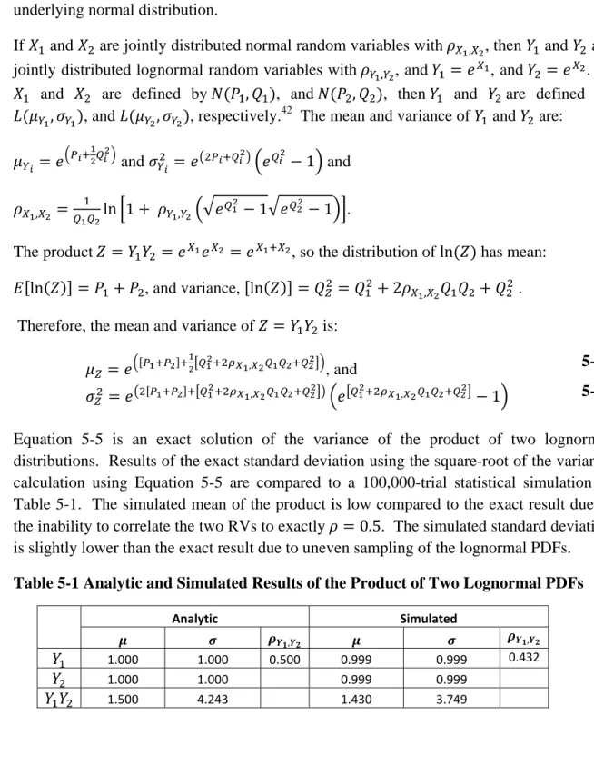
5 Product of Dependent Random Variables... 55
5.1 Product of Two Normal Random Variables ... 55
5.2 Product of Two Lognormal PDFs ... 56
5.3 Product of Exponentiated Lognormal PDFs ... 59
5.3.1 Correlation Between Exponentiated Lognormal PDFs... 60
5.4 Product of Multiple Lognormal PDFs ... 60
5.5 Limitations of Statistical Simulations... 61
6 Mellin Transforms ... 62
6.1 Mellin Transform Properties ... 62
6.2 Mellin Transform of the Uniform Distribution ... 63
6.3 Mellin Transform of the Triangular Distribution ... 63
6.4 Mellin Transform Example ... 63
7 Propagation of Errors ... 67
7.1 Propagation of Errors Example ... 68
v
8.1.1 Type I-1 Functional Correlation Example ... 73
8.2 Type I-2 Functional Correlation ... 75
8.2.1 Type I-2 Functional Correlation Example ... 76
8.3 Type II-1 Functional Correlation ... 84
8.3.1 Common Predecessor Functional Correlation ... 87
8.3.2 Type II-1 Functional Correlation Example ... 88
8.3.3 Type II-1 Functional Correlation between Multivariate Functions ... 90
8.4 Type II-2 Functional Correlation ... 91
8.5 Type III-1 Functional Correlation ... 93
8.6 Type III-2 Functional Correlation ... 95
8.6.1 Type III-2 Functional Correlation Example ... 96
8.7 Section Summary ... 97
9 Discrete Risks ... 98
9.1.1 Single Discrete Risk Case ... 98
9.1.2 Mean of Mixed Distribution ... 100
9.1.3 Standard Deviation of Mixed Distribution ... 101
9.1.4 Multiple Risks Case ... 102
9.1.5 Multiple Discrete Risks Example ... 103
9.1.6 Binary State Representation ... 104
9.1.7 Adding Discrete Risks with Impacts that are Random Variables ... 105
9.1.8 Discrete Risk Numerical Example ... 107
10 Maximum and Minimum of Random Variables ... 110
10.1.1 Maximum and Minimum of Correlated Non-Gaussian PDFs ... 112
11 Example Problems ... 117
11.1 Parametric Estimate Example Problem ... 117
11.1.1 Cost Distribution... 117
11.1.2 Probability Distributions ... 118
11.1.3 Schedule Probability Distribution ... 123
11.1.4 Forming the Joint Distribution ... 124
vi
11.2.2 Cost Probability Distribution ... 152
11.2.3 Joint Cost and Schedule Distribution ... 165
12 Summary ... 171
13 Conclusions and Recommendations ... 172
13.1 Conclusions ... 172
13.2 Recommendations ... 172
13.2.1 Evaluating Statistical Simulations ... 173
13.2.2 Using Estimating Methods ... 173
13.2.3 Basis of Estimate Credibility ... 173
13.2.4 Developing Cost Models ... 173
13.2.5 Improving Cost and Schedule Risk Tools ... 174
13.2.6 Time-Phasing a Resource-Loaded Schedule ... 175
13.2.7 Allocating Schedule Margin ... 175
14 Acronyms, Symbols and Definitions ... 176
14.1 Acronyms ... 176
14.2 Symbols ... 177
15 Bibliography ... 179
16 Appendices ... 182
16.1 Appendix A – Probability Distributions... 182
16.1.1 Uniform Distribution ... 182
16.1.2 Triangular Distribution ... 183
16.1.3 Normal Distribution ... 183
16.1.4 Lognormal Distribution ... 184
16.1.5 Beta Distribution... 185
16.1.6 Bivariate Normal Distribution ... 187
16.1.7 Bivariate Normal-Lognormal Distribution ... 187
16.1.8 Bivariate Lognormal Distribution ... 188
16.2 Appendix B – Expectation Operations ... 189
16.2.1 Expectation Properties ... 189
vii
16.3.1 Derivation of PDF of an Analog... 191
16.3.2 kth Moments of a Triangular Distribution ... 193
16.3.3 Propagation of Errors Derivation ... 195
16.3.4 Derivation of Mean of Mixed Distribution ... 195
16.3.5 Max of Farlie-Gumbel-Morgenstern Joint PDFs... 196
16.3.6 and Parameters for Symmetric Case of PERT distribution ... 198
16.3.7 Derivation of Product of Two Normal RVs ... 199
16.4 Appendix D – Visual Basic Functions ... 201
16.4.1 Lognormal Mean and Sigma ... 201
16.4.2 kth Moment of a Lognormal Distribution ... 201
16.4.3 Mellin Transform ... 201
16.4.4 Standard Deviation from Mellin Transform ... 202
16.4.5 Kurtosis from Mellin Transforms ... 202
16.4.6 Gamma Function ... 202
16.4.7 Uniform Distribution Function ... 202
16.4.8 Moments of Maximum of Two Bivariate Normal Distributions ... 203
16.4.9 Moments of Maximum of Two Bivariate Lognormal Distributions ... 204
viii
ix
ACKNOWLEDGEMENTS
The author wishes to acknowledge the support of the NASA Office of Program Analysis and Evaluation (PA&E), Cost Analysis Division (CAD) for this research. Specific thanks go to Mr. Charles Hunt, Dr. William Jarvis and Mr. Ronald Larson whose enthusiasm in this research resulted in this document.
I would like to acknowledge the significant contributions of my late mentor, Dr. Stephen Book, whose work laid the foundation to this report. I would also like to thank Dr. Paul Garvey (MITRE) and Mr. Timothy Anderson (iParametrics) for their assistance with many of the difficult subjects approached in the report.
I extend my gratitude to Galorath, Inc.: specifically, Mr. Dan Galorath for his gracious assistance in making this work possible; Mr. Robert Hunt for his diligence as the project manager; Mr. Brian Glauser for his promotion of the effort; Ms. Wendy Lee for her help deciphering the elusive properties of the beta distribution; and Ms. Karen McRitchie for her support in motivating the technical application of the analytic method into SEER-H.
x
11
1
Executive Summary
Estimates of cost and schedule duration of a task or project are uncertain values, so we do not know the exact, discrete values until it is complete. Given the inherent uncertainty of estimates, the only way to portray them is with probability distributions of possible costs and schedule durations (or dates). Probabilistic cost and schedule distributions for a program are quantified through the means of cost and schedule uncertainty analyses. The most popular way these analyses are performed is though statistical simulation. Statistical simulation (i.e., Monte Carlo and Latin Hypercube sampling) techniques are widely used in cost and schedule risk analysis, but they have limitations.
Analytic methods of cost and schedule risk analysis exist that: 1) correctly model random variables (RVs); 2) exactly correlate RVs and their sums, which many statistical simulation tools cannot; 3) have no fundamental limit to the number of RVs or correlation coefficients that can be defined; 4) provide [near] instantaneous results; and 5) have the ability due to their mathematical form to clearly indicate uncertainty drivers and thus the risk.
This report presents an analytic (i.e., a non-simulation based) method of quantitative cost and schedule risk analysis building on analytic techniques of applied probability and statistics. The analytic method provides near-instantaneous results with exact statistics such as mean and variance of total cost and total schedule duration. It capitalizes on the fact that the structure of estimates defines a mathematical problem to be solved through the use of applied probability. This report provides the mathematics required to perform the tasks of calculating the uncertainty of an estimate, and determining the risk from this uncertainty and a point estimate.
While much of the mathematics of applied probability used in this report are publicly available through journal publications, the author has derived methods and formulae that have, to his knowledge and through his research, never been published before. Therefore, the report provides a very unique set of mathematics useful in the analytic assessment of cost and schedule uncertainty and risk.
The report includes several quantitative examples, including two example estimates, where the results obtained using the analytic method compare well with those results obtained through statistical simulation. Given the excellent results obtained through this research, additional applications of the analytic method are recommended for use in risk analysis, estimating relationship development, and probabilistic cost and schedule estimating.
12
2
Introduction
This report describes an analytic method of applied probability analysis techniques germane to problems encountered in cost and schedule risk estimation. By their very nature, estimates are uncertain projections of future events. Given that, we discuss the probabilistic nature of estimates and describe the mathematical problems encountered in cost and schedule estimating. We discuss the mathematical tools that can be used to solve these problems (i.e., statistical simulation and statistical analysis) and we compare the two approaches. The next sections of the report provide the tools required to perform statistical analysis. Finally, we provide two sample problems to demonstrate analytical techniques.
2.1 ProbabilisticNatureofEstimates
Cost and schedule estimating is an integral part of the program management process. Organizations use these estimates for planning purposes such as cost/performance tradeoff studies, benefit/cost analyses, source selections, and budget planning. But estimates are predictions and their exact values are uncertain in nature since they have not yet become “fact”. Since the true cost and schedule durations of a project (or task) are only known when it is complete, the best we can do is to rely on estimates at various stages of planning and completion.
The word “estimate” itself implies uncertainty, so an estimate is not well represented by a single number but by a distribution of possible estimates. The distribution of possible estimates is defined by the estimate’s probability distribution that is calculated through the application of probability and statistics.
2.2 UncertaintyandRisk
Uncertainty is a measure of the distribution of possible outcomes of a random variable, such as cost and schedule estimates. This distribution is called a probability distribution and can either be a continuous, discrete, or mixed distribution.1
2.2.1 ProbabilityDensityandProbabilityMass
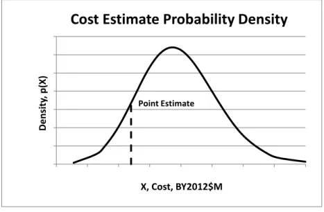
Probability distributions defined for continuous distributions are probability density functions (PDFs). PDFs such as the one shown in Figure 2-1 can be expressed in terms of a mathematical formula of , where is the PDF defined over the range, .
1
13
Figure 2-1 Probability Density Distribution
Probability distributions of discrete risks (which are discontinuous functions) are defined by probability mass functions (PMFs) such as the one shown in Figure 2-2. We will define the PMF as , where is the function defined over the range .
Figure 2-2 Probability Mass Distribution
2.2.2 CumulativeProbability
The cumulative probability is the probability that a real valued random number will be less than some value . In the case of discrete distributions, it is the sum of the probability-weighted values of the PMF less than , and in the case of continuous distributions, (remembering our college calculus) it is the integral of the PDF from – ∞ to .
Point Estimate 0 0.001 0.002 0.003 0.004 0.005 0.006 0.007 400 450 500 550 600 650 700 750 800 Density , p( X ) X, Cost, BY2012$M
Cost
Estimate
Probability
Density
0 0.05 0.1 0.15 0.2 0.25 0.3 0.35 400 425 450 475 500525550575600 625 650 675 700 725750775800 Pr o b ab ili ty Ma ss, f(x) X, Cost, BY2012$M
14
2.2.3 DefinitionofRisk
Any point estimate has some probability that it will be sufficient or be exceeded (Figure 2-3). The probability that an estimate will be exceeded (i.e., overrun) is the risk, and the probability that the estimate will be sufficient (and that there is a probability of the actual value being lower) is the opportunity or reward.
Figure 2-3 Risk, Reward and the Point Estimate
Since the entire area under the PDF shown in Figure 2-3 is, by definition, equal to one, the sum of the probabilities of overrun (risk) and under-run (reward or opportunity) is also equal to one. The probability of risk occurrence is the area of the distribution to the right of the point estimate and the probability of reward is the area to the left. As stated earlier, the area of the distribution under a curve can be computed using the definite integral expression bounded by the lower and upper limits. Therefore, risk is the integral of the PDF from the point estimate, c, to infinity (∞ .
1 1 . 2-1
Reward or opportunity represents the area under the curve from ∞ to c, which is
. 2-2
If we are using discrete risks defined by PMFs, then the risk equation is a summation of all of the probability-weighted risk consequences at all points x (i.e., costs or schedule durations) (Garvey P. R., 2000) greater than our point estimate, .2
∑ . 2-3
2
Garvey, P. R. (2000). Probability Methods for Cost Uncertainty Analysis: A Systems Engineering Perspective. New York, NY: Marcel Dekker.
15
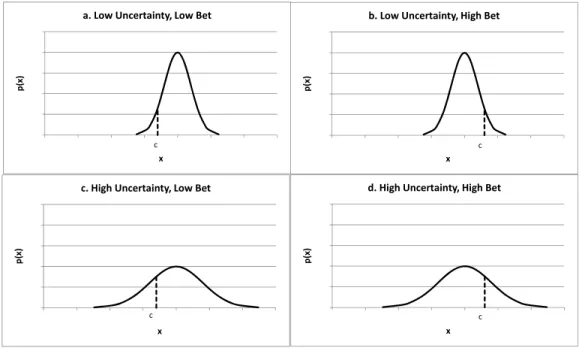
The amount of risk to an estimate is defined by two things: the uncertainty of the estimate and the point estimate, or the bet. To illustrate the interaction of risk with uncertainty and the bet, consider the four examples in Figure 2-4. Figure 2-4a. is a low-uncertainty, high-risk estimate since the area under the PDF to the right of the bet is much larger than that to the left. This means there is a disproportionate amount of risk compared to opportunity. In in Figure 2-4b, the risk is reduced by choosing a bet further to the right in the PDF. Note that in both of these cases, the potential low- and high-end outcomes remain the same – only the bet is changed. When the low bet is accompanied by a larger estimate uncertainty, as in in Figure 2-4c, the risk is reduced, but the potential impacts due to high-end outcomes (consequences) are increased. Finally, moving the bet to the right in the high uncertainty case, the risk is reduced as shown in in Figure 2-4d, but the potential for extreme high-end outcomes remains.
Figure 2-4 Relationship between Risk, Uncertainty and the Bet
2.3 JointProbabilityDistributions
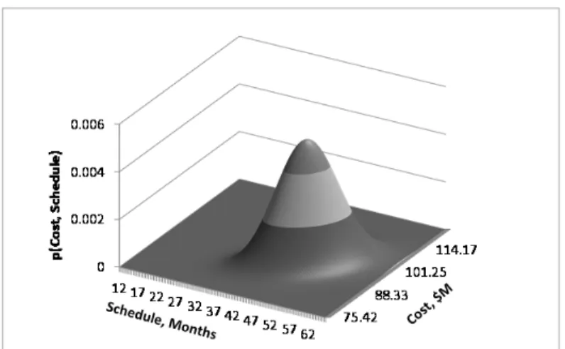
So far we have discussed the univariate3 probability distributions of single random variables (i.e., estimates of cost or schedule). When we are interested in the probability distribution of more than one random variable, we are interested in the multivariate probability distributions, such as the probability of achieving a particular cost and schedule of a yet-to-be-completed project. When the relationships between variables such as estimated cost and schedule must be considered, we need to form a joint probability distribution. An example of this is shown in Figure 2-5.
3 Single variable 0 0.5 1 1.5 2 2.5 0 0.5 1 1.5 2 2.5 3 3.5 p( x) x
a. Low Uncertainty, Low Bet
c 0 0.5 1 1.5 2 2.5 0 0.5 1 1.5 2 2.5 3 3.5 p(x) x
b. Low Uncertainty, High Bet
c 0 0.5 1 1.5 2 2.5 0 0.5 1 1.5 2 2.5 3 3.5 p( x) x
c. High Uncertainty, Low Bet
c 0 0.5 1 1.5 2 2.5 0 0.5 1 1.5 2 2.5 3 3.5 p(x ) x
d. High Uncertainty, High Bet
16
Figure 2-5 Joint Probability Density Function
If we have two random variables and , we can define the probabilities
2-4
The joint probabilities of , can be expressed as the joint distribution function
, , , 2-5
The joint PDF is defined as the partial derivative of , with respect to and .
, , 2-6
2.3.1 MarginalDistributions
The marginal distributions of a joint probability function are those distributions that are considered individually. Given a joint distribution of two random variables, the marginal distribution of one is its probability distribution averaged over the probability information from the other’s distribution.
2.3.2 ConditionalDistributions
A conditional distribution of a joint probability function is the distribution of one random variable given a specific value of the other distribution(s).
17
2.4 StatisticsofaRandomVariable
2.4.1 Moments
Moments provide useful information about the characteristics of a random variable, , such as the measures of central tendency, dispersion and shape. When referring to the moments of a distribution or a set of data, it is useful to define which of the three types of moments are being used: raw moments, central moments or standardized moments.
2.4.1.1 Raw Moments
The kth moments about the origin are called “raw moments” of a PDF, , and are defined as:
∑ ;
;
2-7
The mean, , is the first raw moment of about the origin, and it is a measurement of the central tendency of the data. We are more familiar with the mean being represented as, , so we will use this notation for the mean hereafter.
2.4.1.2 Central Moments
Central moments of a distribution are the raw moments about the mean, . The first central moment is by definition zero, but the second central moment is the variance, , which is a measure of dispersion about . Equation 2-8 provides the definition of the kth
central moments of discrete and continuous RVs.
∑ ;
;
2-8
The variance, , is the square of the standard deviation, .
The first five central moments expressed in terms of the raw moments are:
0 2-9 2-10 2 3 2-11 3 6 4 2-12 4 10 10 5 2-13 2.4.1.3 Standardized moments
Standardized moments are the kth central moments, , normalized by the kth powers of the standard deviation (i.e., ).
18
The most well-known standardized moments are skewness and kurtosis. Skewness, , is the measure of asymmetry of and is defined as the third standardized moment:
2-14
A distribution is a) symmetric if 0 , b) left (i.e. negatively) skewed if 0 , and c) right (i.e., positively) skewed if 0 as shown in Figure 2-6.
Figure 2-6 Left and Right Skewed Distributions
Kurtosis is the fourth standardized moment. Most textbooks define kurtosis of symmetric, unimodal distributions as a measure of peakedness of a distribution . This is a correct definition, however a more descriptive definition of kurtosis exists (DeCarlo, 1997), (Moors, 1986), (Balanda & MacGillivray, 1988), and (Darlington, 1970).4, 5, 6, 7 Moors defines kurtosis as the measure of the dispersion around the two “shoulders” of a distribution located at . DeCarlo warns that the classical attribution of peakedness of a distribution vice its “fat-tailedness” is not a good representation of the meaning of kurtosis and provides examples where this is the case.8
2-15
A more commonly used metric is the “excess kurtosis”, which is 3. Since the kurtosis of a normal distribution is equal to three, the excess kurtosis denoted as , is adjusted by 3 as in Equation 2-16.
3 3 2-16
In general, where a) 0 the distribution is mesokurtic, b) 0 it is leptokurtic, and c) 0 it is platykurtic.
4
DeCarlo, L. (1997). On the meaning and use of kurtosis. Psychological Methods, 292-307.
5
Moors, J.J.A. The meaning of kurtosis: Darlington reexamined. Amer. Statist.1986, 40, 283-284.
6
Balanda, K.P.; MacGillivray, H.L. Kurtosis: A critical review. Amer. Statist.1988, 42, 111-119.
7
Richard B. Darlington. Is Kurtosis Really "Peakedness?". Amer. Statist. 1970, 24, 19-22.
8
19
Figure 2-7 Excess Kurtosis of Distributions
2.4.1.4 Moment Summary
The moments describing the characteristics of a random variable such as the measures of central tendency, dispersion and shape (i.e., , , , ) can be derived from the raw moments of . We will capitalize on these relationships in the analytic method proposed in this report.
2.4.2 QuantileStatistics
Quantiles are a set of divisions of data into groups containing equal numbers of observations. We are most familiar with percentiles, which are division of the data into 100 groups of 1% of the cumulative area under a PDF. We will denote the percentile, , of a random variable, , as . For example the 50th percentile of would be written . .
2.4.3 ExpectationOperator
The expectation operator, ∙ , of a random variable is a powerful expression. The expected value, or , (Equation 2-17) of a random variable is perhaps the most important single parameter in applied probability. It is written as
, 2-17
and is the integral
, where is the PDF of . 2-18
The mean represents the center of gravity of the random variable. Another important parameter is , defined by the expectation of the squared difference of the PDF and its
20
mean. This quantity represents the moment of inertia of the probability masses (Papoulis, 1965).9
2-19
What is most important about ∙ is its ability to determine the raw moments (Equations 2-7 and 2-18) and central moments (Equations 2-8 and 2-19) of a random variable, and thus the measures of central tendency, dispersion and shape (i.e., , , , ).
2.4.4 OrderStatistics
Order statistics are those statistics that describe the numerical order in which random variables or samples of random variables appear. Some of the simplest order statistics are the minimum and maximum values defining the range of a PDF. Other, more complex order statistics are those which describe the maximum and minimum of a series of random variables. Order statistics play an especially important role in schedule risk analysis whereby the maximum probabilistic end dates of certain tasks define the maximum probable end-date of the schedule.
2.5 SectionSummary
The mathematics of the analytic techniques used to solve estimating uncertainty problems require definition of the estimating problems germane to cost and schedule estimates. In the next section, we discuss the mathematical problems typically found in cost and schedule estimating.
9
Papoulis, A. (1965). Probability, Random Variables and Stochastic Processes. New York, NY: McGraw Hill.
21
3
Cost and Schedule Estimates
Cost and schedule estimates are defined by a set of mathematical formulae that lend themselves to probabilistic uncertainty analysis. In this section, we will discuss the structures of these types of estimates and define the mathematical problem(s) to be solved in probabilistic uncertainty analysis.
Book10,11 (1994; 2002) showed the cost and schedule estimating communities that every cost and schedule estimating problem should be treated as a risk analysis, not simply an exercise in summing most likely costs – the result of which is a number that has no statistical meaning without risk analysis. Furthermore, he showed estimates should be treated as random variables and not deterministic numbers (i.e., constants).
3.1 Nomenclature
To better describe the mathematical problems germane to cost and schedule estimates, we will define constants, variables, and random variables.
A numerically expressed entity is called a “constant” if there is a unique specific number that is always its numerical value (e.g., , 1.414, -2). A numerically expressed entity is called a “variable” if there are several possible specific numbers that may serve as its numerical value and which specific number happens to be its numerical value in any particular situation depends on the particular circumstances (e.g., , , )12. A variable is further denoted a “random variable” if the proportion of particular situations in which any specific number happens to be its numerical value is established by a probability distribution (e.g., , , cost, schedule duration).
We will use the following notation throughout this document to define variables. Constants will be defined using their numerical value or lowercase letter (e.g., , , , , ). Variables will use lowercase letters , , , , , and , and random variables will use uppercase letters , , , , and . Random variables defined by commonly used PDFs will use the following notation:
Uniform: ; , , 3-1 Triangular: ; , , , , 3-2 Normal: ; , , 3-3 Lognormal: ; , , 3-4 Beta: ; , , , , , , 3-5 Where 10
Book, S. A., “Do Not Sum ‘Most Likely’ Cost Estimates”, 1994 NASA Cost Estimating Symposium, Johnson Space Center, Houston, TX, 8-10 November 1994.
11
Book, S. A., “Schedule Risk Analysis: Why It is Important and How to Do It”, Ground Systems Architectures Workshop, The Aerospace Corporation, El Segundo, CA, 13-15 March 2002.
12
22
L, M, H are low, most likely (mode), and high shape parameters
, are the mean and standard deviation of the distribution in unit space α, β are standard beta distribution shape parameters
a, b are lower and upper bounds of the four-parameter beta distribution
The properties of these distributions are provided in Appendix A – Probability Distributions.
3.2 TheCostEstimatingProblem
The cost estimating problem is defined by the mathematics of the following: 1) the work breakdown structure (WBS), which requires multiple levels of statistical summation; and 2) the mathematics most applicable to the estimating approach(es) used (i.e., bottom-up, analogy, parametric). We will first describe the statistical techniques used to perform statistical summation of a WBS structure and then discuss, in more depth, how to apply analytic uncertainty and risk analysis to the individual WBS elements.
3.2.1 WBSstructure
The WBS defines the summation hierarchy of the project. In other words, it defines the mathematical problem of summation of individual WBS elements to successively higher levels of the WBS up to the total project level. The statistical treatment of summing correlated random variables is fairly straightforward and can be easily programmed into a spreadsheet or cost estimating tool (Young, 1992).13
3.2.2 EstimatingMethods
The methods used to estimate costs at different WBS levels define another part of the mathematical problem to be solved. Different estimating methods require different mathematical procedures, so we will examine these methods individually and note the important mathematical features of each. These include bottom-up, analogy approach relying on scaled actuals, multiple scaled actuals, and cost estimating relationships (CERs).
3.2.2.1 Bottom-up
The bottom-up estimating approach relies on summing a detailed list of the classical elements of cost: labor (effort), material and expenses. If a detailed, resource-loaded schedule is used to estimate effort, then the duration of the task, the staffing level and the associated labor rates can be represented by random variables. As an example, the cost of
13
The “Formal Risk Assessment of System Cost Estimates” (FRISK) method is an analytic risk model that uses “Method of Moments” to calculate summary distributions. FRISK was originally developed by Phil Young of The Aerospace Corporation in 1992 (before Crystal Ball and @Risk became available) with funding from USAF SMC. A BASIC Program implementing FRISK was developed by Dr. Stephen Book and enjoyed many years of use. FRISK has been reprogrammed in Excel by various analysts since 2000, with each new version providing more advanced capability and features and ease of use.
23
the effort for a particular task is the product of the task duration, the resource loading profile and the associated labor rates. Each is treated as a random variable.
; where
= effort, measured in dollars
= duration of the task, measured in hours = resource loading, measured in heads
= the labor rate, measured in dollars per hour per head
In this case, the first mathematical problem to be solved is the multiplication of multiple (and perhaps correlated) random variables. This will be discussed in Section 5. The second problem is the summation of the elements of cost represented by random variables for each WBS element, as discussed in Section 4.2.2.
3.2.2.2 Analogy (Scaled Actuals)
The analogy method relies on using an actual cost of a product or service to estimate the cost of a similar product or service. Intuitively, it is the easiest method to use when preparing a cost estimate. The simplest form of an analogy estimate is a direct analogy, in which case the estimated cost is equated to the actual cost of the similar product or service. Unfortunately, this simple procedure does not provide any information about the uncertainty of the estimate. Indeed, the analogy can be the most misleading estimating method from a probability perspective.
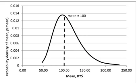
Studies (MacKenzie & Addison, 2000) by the Space Systems Cost Analysis Group (SSCAG) have shown the standard deviation of the costs of similar items at the “box level” of the WBS to be as much as 30% to 40%.14 In the same report, the authors showed the data to be lognormally distributed, which provides a shape to the distribution. Given this information, we are able to derive a measure of the standard deviation of the “actual” cost based on the coefficient of variation ( / ), but we do not know at which percentile to place our particular analogy. Is it at the 50th percentile (median), the mode, the mean (expected value), or is it at some other percentile such as the 4th or the 85th, or somewhere else? If it is at the mean, then the PDF of the analog is easily determined. But, is this the right PDF to use in this situation? Figure 3-1 shows an example lognormal distribution based on the mean and 0.3, 100, 30 .
14
MacKenzie, D. and Addison, B., “Space System Cost Variance and Estimating Uncertainty”, 70th SSCAG Meeting, Boeing Training Center, Tukwila, WA, October 12-13, 2000.
24
Figure 3-1 PDF of Cost of Analogy at Mean
Now consider the case where the analogy is one cost of many possible costs within an unknown probabilistic range. To provide a distribution about the analogous cost, we need to either 1) assume a percentile value for the analogy within a prescribed distribution, or 2) determine the (yet unknown) probabilistic range of possible values to which the analogous cost belongs. The first case is described by Flynn, Braxton, Garvey and Lee (2012).15 The second case requires the use of applied probability to determine the probability distribution. The derivation for this approach is provided in Appendix C – Derivations.
3.2.2.3 Scaled Actuals (Factor)
If a simple factor is used to scale an actual cost, then the mathematical problem is the multiplication of random variables, where one random variable is the scaling factor and the other is the PDF of the analogy, described in Section 3.2.2.2.
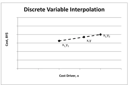
3.2.2.4 Scaled Actuals (Interpolation)
When we estimate the cost of an item through linear interpolation of two actuals using a cost driver (i.e., weight), the mathematical problem is a linear relationship:
∗ , where 3-6
= the cost estimate (random variable)
= the cost driver of the item we are estimating (a random variable) , = the costs of the two actuals, (random variable)
, = the cost drivers of the two actuals (constant)
15
Flynn, B., Braxton, P., Garvey, P., & Lee, R. (2012). Enhanced Scenario-Based Method for Cost Risk Analysis: Theory, Application and Implementation. 2012 SCEA/ISPA Joint Annual Conference & Training Workshop. Orlando, FL. mean = 100 0 0.002 0.004 0.006 0.008 0.01 0.012 0.014 0.016 0.00 50.00 100.00 150.00 200.00 250.00 P ro b ab ilit y dens ity of mea n , p(me an) Mean, BY$
25
The plot of the discrete interpolation problem is shown in Figure 3-2.
Figure 3-2 Discrete Variable Interpolation
The mathematical problems to be solved in Equation 3-6 are the addition, subtraction and multiplication of random variables.
Note the costs of the two actuals have a similar issue as the direct analogy method whereby we cannot assume the a priori standard deviations of the samples. If we cannot treat these samples of actual values as constants (no error) in the direct analogy case, then we shouldn’t treat them as such in the interpolation case.
3.2.2.5 Multiple Scaled Actuals and Cost Estimating Relationships
Multiple scaled actuals are those actuals that are similar in nature and whose costs can be represented by a probability distribution or by simple moments such as and . For example, the costs of three-meter ground station antennas could be represented by a normal distribution, , . Provided the antenna of interest fits into the set of three-meter ground station antennas represented by the PDF, we know the , , and confidence level of each estimate in the range of the PDF.
When we are estimating costs of products or services that are based on a similar set of parameters, we can develop a cost estimating relationship (CER) that explains some of the variations in cost based on variations in one or more independent variables (i.e., cost drivers). Consider the generic form of a recurring CER based on unit theory shown in Equation 3-7.
∑ ∏ ∏ ; where
, , , , and are coefficients of the regression ( ), = cumulative average learning curve slope when a = 0, = unit number , 3-7 0 2 4 6 8 10 12 0 0.5 1 1.5 2 2.5 Co st , BY $ Cost Driver, x
Discrete
Variable
Interpolation
x1,y1
x2,y2 x,y
26 = independent variable ,
= number of independent variables, = indicator (“dummy”) variable , = number of indicator variables, and = percent standard error (multiplicative).
The independent variables, , can be represented by random variables as can the multiplicative error of the estimate, . The dependent variable, , will also be a random variable, , defined by the PDFs of each independent variable, the functional transformation of the CER form, and the PDF of the multiplicative error, .
The CER provides a model for constructing the PDF, so we can obtain the , , and confidence level of each estimate in the range of the PDF as in the case of multiple scaled actuals. To compute the statistics of the CER, we must first learn how to convolve and transform random variables. This is discussed in Sections 4 through 7.
3.2.3 DiscreteRisks
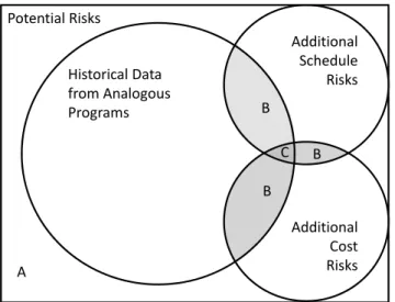
Analysts may need to include discrete risk events form a risk register (Table 3-1) in a cost or schedule estimate. In the single risk case, this means there is a probability that some estimate of additional cost or schedule will be added. With multiple risks, the problem becomes combinatoric, since we must account for any combination of risks that could potentially occur.
Historical cost and schedule actuals contain realized risks which may or may not have been mitigated or manifested themselves into cost and schedule growth from the original proposed estimate. By using historical actuals to form the estimating relationships, the resulting estimate 1) will appear more conservative than if it had been developed using engineering judgment or non-metric-based approaches; 2) will inherently contain schedule and cost risks typical of similar programs; and 3) will be more prone to double or even triple-counting risks when augmented with discrete cost and schedule risks from a risk register (Table 3-1).
Table 3-1 Example Risk Register
Risk ID Description Probability Impact Impact Area
R1 Additional program management personnel 0.50 $200,000 Cost
R2 Redesign of computer board 0.25 6 Months
$75,000
Schedule Cost
R3 Parts failure 0.10 $250,000 Cost
Technical
R4 Second vendor required 0.05 12 months Schedule
Technical
27
To form a complete risk picture, additional cost-related risks identified by the schedule risk assessment (SRA) and the discrete risk analysis obtained from the risk and opportunities register (ROR) are included to form the risk profile of the program. In many cases, the historical risk inherent in the use of estimating methods developed from actual data covers many potential risks (Figure 3-3). In these cases, the analyst must identify unique risks and omit redundant risks (B and C) identified and represented in the SRA and ROR. The use of more robust statistical and risk analyses minimizes the unidentified and untracked risks (A).
Figure 3-3 Estimating Risk Venn Diagram
3.3 TheScheduleEstimatingProblem
The schedule estimating problem is defined by the method used to estimate the schedule duration. When scaled analogy or multiple scaled actuals or schedule estimating relationships (SERs) are used to estimate schedule duration, the mathematical problem to be solved is similar to those of cost estimating. The two fundamental differences are: 1) probabilistic durations are measured in workdays, and 2) when the bottom-up approach is used, the schedule network defines the mathematical problem to be solved. We will discuss the issues that arise when using workdays rather than calendar days and then discuss the issues arising from the arrangement of tasks in a network.
3.3.1 UsingWorkdaysinaSchedule
When using workdays in a program schedule, probabilistic dates are expressed as discrete rather than continuous distributions. This arises from the fact that a particular task may finish on a particular day (or part of a work day) but not all possible values within the range. Consider the example of the duration of a task to be a continuous, uniform distribution defined as 1,2 . The lower bound of the continuous distribution is defined as one day and the upper bound as two days. Assuming a continuous distribution for the duration of the task, the finish date of the task will be within the range of one to two days
Historical Data from Analogous Programs Potential Risks Additional Schedule Risks Additional Cost Risks B B B C A
28
later. In our example, the mean and standard deviation of the duration’s continuous uniform , distribution are:
, 1.5 days
, 2 1 0.2887 days
Since schedules (and scheduling software programs) use discontinuous working days (as opposed to continuous calendar days) to define start and finish dates, the probabilistic finish date will be one or two days after the start date, not anywhere within entire range of the distribution. This phenomenon induces changes in the statistics of the finish date of the task and the overall distribution shape and statistics of the schedule. If the duration is treated as a discrete uniform , distribution with two (n=2) discrete days duration, the statistics are:
, 1.5 workdays (wd)
, , , . . 0.5 wd
Note the mean is unchanged, but the variance increases dramatically because the probability mass is equally distributed at the lower (L) and upper (H) bounds of the distribution. The statistics take a more severe departure when evaluating the distribution in calendar days where one possible finish day may occur on a Friday and another on a Monday, assuming Saturday and Sunday are not workdays. This translates into a distribution with two possible durations in calendar days with the statistics:
, 2.5 calendar days (cd)
, , , . . 1.5 cd
We must take great care to properly define the appropriate units and respective shapes of durations or else we may be miscalculating the correct moments of the schedule durations, start dates and finish dates. For this reason, probabilistic workdays are defined by continuous distributions, and calendar days are defined by discrete distributions.
3.3.1.1 Converting Calendar Days to Workdays
Scheduling software makes provisions for converting from a number of calendar days to workdays and vice versa. A simple approximation that can be used is:
29
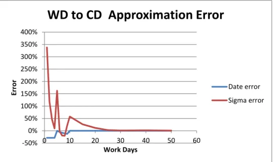
This conversion provides less than 1% error for date conversions over 10 wd as shown in Figure 3-4. An equally useful approach when using Excel is to compute the finish date (in cd) using the WORKDAY() function, which calculates the finish date (in cd) using the start date (in cd) and duration (in wd). The duration in cd (and the appropriate conversion factor from wd to cd) can be calculated by subtracting the finish date (in cd) from the start date (in cd).
3.3.1.2 Expressing Durations and Dates as Random Variables
When probabilistic schedule network tools use continuous distributions to define the probabilistic durations of tasks, they effectively transform the continuous distributions into discrete distributions binned into possible working days. This discretization of continuous distributions scales the standard deviation of the task’s duration. The conversion factor shown in 3-8 provides a good approximation of this scaling for standard deviations of durations over 25 wd as shown in Figure 3-4.
Figure 3-4 Workday-to-Calendar Day Approximation Error
3.3.2 ArrangementofTasksinaNetwork
Schedule networks contain the task durations and the arrangement of those tasks with respect to each other. There are four possible arrangements: serial, parallel, tree and feedback (Book S. A., 2011).16
16
Book, S. A., “Schedule Risk Analysis: Why It is Important and How to Do It”, 2011 ISPA/SCEA Joint Annual Conference & Training Workshop, Albuquerque NM, 7-10 June 2010.
‐50% 0% 50% 100% 150% 200% 250% 300% 350% 400% 0 10 20 30 40 50 60 Error Work Days
WD
to
CD
Approximation
Error
Date error Sigma error30
3.3.2.1 Serial Arrangement
In a serial arrangement, each task is arranged as a predecessor or a successor of another. Figure 3-5 shows a serial arrangement of tasks represented by boxes. The number in each box indicates the duration (number of wd) allocated to the individual tasks. The serial network’s critical path passes through all of the boxes, and its duration is the sum of the durations of the individual activities in the serial network. The critical path, in this case, has a total duration equal to 32 wd.
Figure 3-5 Serial Network (Book S. A., 2011)
3.3.2.2 Parallel Arrangement
In a parallel arrangement, two activities are “parallel” if neither is a predecessor or a successor of the other. The critical path passes through those boxes whose combined duration is the longest possible through the network, not the sum of the durations of all of the individual tasks in the network.17 In Figure 3-6, the series of tasks on the top (the critical path) is outlined in solid lines and have a total duration of 32 wd; the series of tasks at the bottom is outlined in dashed lines and has a total duration of 27 wd.
Figure 3-6 Parallel Network (Book S. A., 2011)
3.3.2.3 Tree Structure
A tree structure is a mixture of serial and parallel activities in a schedule network. In Figure 3-7, the numbers in boxes indicate number of workdays allocated to the task represented by each box. The critical path passes through those boxes whose combined duration is the longest possible through the network, not the sum of the durations of all of the individual tasks in the network. The critical path, consisting of boxes outlined in solid lines, has a total duration = 25 wd. The sequences of boxes outlined in dotted black lines have “slack time” of 3 wd, 8 wd, 21 wd, 5 wd and 1 wd, respectively.
17
The fundamental reason why “Earned Schedule” is an incorrect approach for estimating the expected duration of a program with parallel paths is that the total schedule duration is not equal to the sum of the individual task durations.
3 1 6 2 3 4 2 2 1 8
3 1 6 2 3 4 2 2 1 8
31
Figure 3-7 Tree-Structured Network (Book S. A., 2011)
The critical path in this case is defined by the maximum of the path durations of each “branch” or path in the tree structure. This is a fundamental difference between schedule-analysis software and cost-schedule-analysis software. The work breakdown structure is a “linear” list, and program cost is calculated by adding together the costs of all items on that list. The schedule network (unless it is entirely serial) is not linear, and therefore program duration cannot be calculated by adding together the durations of all activities in the network.
3.3.2.4 Merging Tasks
When parallel branches or tasks in a tree structure merge, the start date of their successor task is driven by the maximum of the end dates of the merging predecessor tasks. The mathematical problem to be solved when dealing with probabilistic schedule analysis (i.e., probabilistic start dates, end dates and durations) where tasks merge is the calculation of the PDF of the maximum, , of the PDFs of merging tasks (Covert, Using Method of Moments in Schedule Risk Analysis, 2011). This is the source of a phenomenon called “merge bias” which was first discovered in the early 1960s (MacCrimmon & Ryavec, 1962), (Archibald & Villoria, 1967) when a statistical approach was applied to schedule network analysis.18,19
3.3.2.5 Feedback Loop
A feedback loop uses a series of feedback paths to define repeated paths such as repeated testing due to test failures and subsequent fixes. In Figure 3-8, the numbers in boxes indicate the number of wd allocated to the task represented by each box. The critical path passes through those boxes whose combined duration is the longest possible through the network. If “feedback” is not exercised, the critical path, consisting of the boxes outlined in solid lines, has a total duration = 19 wd. If “feedback” is exercised once, all boxes lie on the critical path, which then has total duration = 44 wd.
18
MacCrimmon, K. R., & Ryavec, C. A. (1962). An Analytical Study of the Pert Assumptions. Santa Monica, CA: RAND.
19
Archibald, R. D., & Villoria, R. L. (1967). Network-Based Management Systems (PERT/CPM). New York: John Wiley & Sons.
3 5 3 2 4 1 3 5 2 2 6 4 5 3 7 4 1 3 3 4
32
Figure 3-8 Feedback Loop (Book S. A., 2011)
3.3.2.6 Probabilistic Branching
The feedback loop is difficult (and sometimes impossible) to model using commercially available scheduling software, and is often modeled using probabilistic branching techniques. These techniques insert a series of tasks in a schedule network with a set of enabling “switches” based on the probability that these additional or repeated tasks will occur. In Figure 3-9 , the probabilistic switches are indicated by circles (nodes) containing “ ”, representing the probability of the path being exercised.
Figure 3-9 Feedback Loop with Probabilistic Decisions
Written in a non-recursive form, the additional, repeated tasks look like those shown in Figure 3-9.
Figure 3-10 Feedback Loop with Probabilistic Branching
Probabilistic branching requires us to know how to add probability-weighted schedule duration (a random variable) to a particular path’s duration (another random variable) (Covert, Using Method of Moments in Schedule Risk Analysis, 2011).
3.3.3 TheCriticalPath
The criticality index ( ) is the probability a particular task’s path will be on the critical path, or the probability one path will have a longer duration than the others. Where three parallel paths ( , and ) with probabilistic end dates merge, there are three potential critical paths, each with its own , defined as:
, 3 5 2 2 1 4 5 1 3 4 3 5 2 2 1 4 5 1 3 4 p p 3 5 2 2 1 4 5 3 4 p p 2 2 1 3 5 2 2 1 1
33 ,
,
Generally, we can state the of path ( ) to be
3-9
Using the notation for the maximum of distributions to be X, then the probability that the end date of path A is greater than the maximum of paths B and C, P(A>X), which is the same as P(X<A), and therefore P(X-A<0). We will need to know how to subtract two correlated random variables (the probabilistic durations of the individual paths in the network) to compute the CI (Covert, Using Method of Moments in Schedule Risk Analysis, 2011).20
3.4 MathematicsofEstimates
In Sections 3.2 and 3.3, we discussed mathematical problems to be solved when using a variety of cost and scheduling estimating methods. The mathematical operations applied to random variables in which we are most interested are (Figure 3-11): addition and subtraction, multiplication and division, correlation between random variables, minimum and maximum, linear and nonlinear transformations, and discrete risks and probabilistic branching. These operations between PDFs result in new PDFs with moments of their own, which we will use in the analysis. What we have not discussed yet is the subject of correlation of random variables, which affects all of these operations.
Figure 3-11 Mathematics of Random Variables
20
34
3.4.1 CorrelationbetweenRandomVariables
When performing operations on random variables we must have knowledge of how they behave with respect to each other, or covary. Correlation is a statistical measure of association between two random variables and is specified by a correlation coefficient ( , ). It measures how strongly the random variables are related, or change, with each
other. If two random variables tend to move up or down together, then they are said to be positively correlated. If they tend to move in opposite directions, they are said to be negatively correlated. The most common statistic for measuring association is the Pearson (linear) correlation coefficient, . Another is the Spearman (rank) correlation coefficient, , which is used in statistical simulation tools such as Crystal Ball and @Risk. These two definitions of correlation are different, and should not be confused to mean the same thing. Garvey (1999) pointed out that simulations relying on rank correlation do not correctly model the covariance of random variables.21
Pearson product-moment linear correlation, , , measures the extent of linearity of a relationship between two random variables. It plays an explicit, well-defined role in establishing the sigma value (as well as the range) of the total-cost distribution as described by Book (1994). For example:
, 1 if and only if (iff) X and Y are linearly related, i.e., the least-squares linear relationship between X and Y allows us to predict Y precisely, given X
, = proportion of variation in Y that can be explained on the basis of a least-squares linear relationship between X and Y
, 0 iff the least-squares linear relationship between X and Y provides no ability to predict Y, given X
The second type of correlation, called Spearman rank correlation, , , measures the extent of monotonicity of a relationship between two random variables. Since it does not appear explicitly in the formulae for any of the mathematical operations for which we are concerned, its impact on sigma is not known.
, 1 iff the largest value of X corresponds to the largest value of Y , the second largest, ... , etc.
, 1 iff the largest value of X corresponds to the smallest value of Y, etc.
, 0 iff the rank of a particular X among all X values. In this case it provides no ability to predict the rank of the corresponding Y among all X values
21
Garvey, P. R. (1999). Do Not Use Rank Correlation in Cost Risk Analysis. 32nd DOD Cost Analysis Symposium.
35
Linear and rank correlations are different for different sets of pairwise data. As an example, Figure 3-12 shows the linear and rank correlation coefficients for different plots of x and y variables.22
Figure 3-12 Linear vs. Rank Correlation
We discuss these two types of correlation because: 1) Pearson product-moment correlation is an essential element used to find the distributions formed by mathematical operations on random variables, 2) Spearman correlation is used nearly exclusively in statistical simulations and does not define covariance, and 3) we need to know the difference between them if we are interested in comparing analytical results to those produced by statistical simulations.
3.4.2 CalculatingCorrelationCoefficients
The correlation coefficient between lists of values of random variables, such as the multiplicative (or additive) error terms of CERs, can be calculated quite easily. Previous papers by the author (2001), (2002), (2006) have demonstrated this application. 23, 24, 25 The Pearson product-moment correlation between discrete values such as pair-wise CER residuals is calculated using Equation 3-10.
, ∑ ∑ ∑ 3-10 22
Covert. R. P. (2011). Using Method of Moments in Schedule Risk Analysis. Bethesda, MD: IPM.
23
Covert, R. P. (2001). Correlation Coefficients in the Unmanned Space Vehicle Cost Model Version 7 (USCM 7) Database. 3rd Joint ISPA/SCEA International Conference. Tyson's Corner, VA.
24
Covert, R. P. (2002). Comparison of Spacecraft Cost Model Correlation Coefficients. SCEA National Conference. Scottsdale, AZ.
25
Covert, R. P. (2006). Correlations in Cost Risk Analysis. 2006 Annual SCEA Conference. Tysons Corner, VA.
36
where and are CER residual pairs,
and are individual program residual data, and and are the means of the residuals respectively.
If the two variables exactly follow a linear relationship (with no scatter), then the correlation coefficient , = +1 or -1. Similarly, if there is no correlation between and
, then the numerator should be zero, and , 0.
3.4.3 Correlation,DependenceandIndependence
In the process of researching the analytic method presented in this paper, we found correlation can be induced between two vectors of sampled, uncorrelated variables and when one, the other, or both are transformed through a non-linear equation (i.e., a CER) form such as , or a triad type of CER, .
Consider the two uncorrelated random variables and shown in Table 3-2. We will introduce a linear transformation, 2 3 , and two exponential transformations,
and . A linear transformation does not change the fundamental correlation, as seen in the correlation coefficients , and , (Table 3-3). Small amounts of correlation are induced by the exponentiation of the uncorrelated random variables U and V as seen in , 0.0088, and , 0.1925. Variables correlated with their squares
show a decrease in their correlation from 1.0 as seen in , 0.9811 and , 0.9990.
Table 3-2 Transformed Random Variable Samples
U V W=2+3U X=U2 Y=V2
1 4.2 4 1 17.64
2 2.1 6 4 4.41
3 1.8 8 9 3.24
4 2.2 10 16 4.84
5 4.15 12 25 17.2225
Table 3-3 Correlations between Transformed Random Variables
U V W X Y U 1.0000 0.0000 1.0000 0.9811 ‐0.0088 V 0.0000 1.0000 0.0000 0.1924 0.9990 W 1.0000 0.0000 1.0000 0.9811 ‐0.0088 X 0.9811 0.1924 0.9811 1.0000 0.1828 Y ‐0.0088 0.9990 ‐0.0088 0.1828 1.0000
37
This demonstration shows that while any pair of sampled vectors of random numbers may themselves be uncorrelated, their exponentiated values are not (i.e., , , . While
we may believe we have two sample vectors of independent random variables, we probably do not. True statistical independence is a high standard of independence between random variables and is difficult to achieve – particularly through statistical sampling. A less stringent type of independence is “expectation independence”, in which the variables remain uncorrelated (i.e., , , 0 for any higher order of expectation operations. “Uncorrelated” is the least stringent standard, and as our demonstration shows, correlation can be induced through exponentiation of the random variables.
Another way RVs can be correlated is through the structure of the mathematical problem (i.e., the functional relationship to each other directly through one equation or indirectly through more than one equation), whether that structure is a cost estimate or a schedule network. In a cost estimate, two CERs can be correlated through sharing a common cost driver or where one CER drives another CER, such as a cost-on-cost factor. Garvey26 (2000) provides an analytic method of determining , when and are random variables representing the estimates from errorless CERs. In a schedule network, two finish dates may have uncorrelated durations of their predecessor tasks, but will still be correlated to each other by sharing a common predecessor. We are interested in calculating functional correlation out of necessity when using analytic methods of uncertainty analysis.
26
Garvey, P. R. (2000). Probability Methods for Cost Uncertainty Analysis: A Systems Engineering Perspective. New York, NY: Marcel Dekker.
38
4
Probability Tools
When we use a cost model to perform a cost risk analysis, we need to know the uncertainty of the individual cost estimates, their statistical dependencies, and how to calculate their sums. We can employ statistical modeling techniques such as statistical simulation or statistical analysis to find these uncertainties and their properties. Although the goal is the same, these techniques differ, which we will discuss in more detail.
4.1 StatisticalSimulation
Statistical simulation is a numerical experiment designed to provide statistical information about the properties of a model driven by random variables. It is often used in cost and schedule risk analysis to model the complex interaction of the transformations and summations involved with correlated random variables.
The statistical simulation process follows these steps:
1) Define numerical experiment (spreadsheet, schedule network, etc.) 2) Define PDFs for each random variable
3) Define correlation coefficients for random variables 4) Determine the number of experimental trials
5) For each trial:
a. Draw correlated random variable(s) from defined PDF(s) i. Sample uniform distributions, 1,0
ii. Transform each 1,0 to the desired PDF based on an inverse transformation of the cumulative density function (CDF), denoted as CDF-1.
iii. Correlate the set of PDFs b. Compute the experimental result(s) c. Save the experimental result(s)
6) At the end of the simulation, determine the statistics from the experimental results
4.1.1 SamplingTechniques
Statistical simulation tools use one or more of the following sampling techniques:
Bootstrap sampling: Re-sampling with replacement from sample data numerous times in order to generate an empirical distribution of a statistic
Monte Carlo sampling: New sample points are generated without taking into account the previously generated sample points
Latin Hypercube sampling: Each variable is divided into m equally probable divisions and sampling is done without replacement for each set of m trials
Orthogonal sampling: This adds the requirement that the entire sample space must be sampled evenly
The most commonly-used statistical simulations use Monte Carlo or Latin Hypercube sampling of correlated random variables. The reasonableness of the simulation results
39
depends on the reasonableness of the user inputs, correct modeling of PDFs for all random variables, and the correct specification of the correlation between these PDFs (even if it is assumed to be 0). The accuracy of the simulation is highly dependent on the simulation’s ability to draw uniformly-distributed random variables 1,0 in step 5.a.i and to correlate them correctly in step 5.a.iii.
4.1.1.1 Generating PDFs from Random Number Generators
A random number generator, such as the Excel RAND( ) statement, produces a uniformly-distributed pseudo-random number between 0 and 1 (0 0,1 , 1). We know that the range of the CDF, , for any random number is the same (i.e., 0 1). Based on that knowledge, the uniform draw can be transformed by the inverse of the CDF, the CDF-1, to get the desired probability distribution, as shown in Figure 4-1. The Excel statements are fairly simple to use for this purpose, as we will demonstrate.
We can generate different PDFs using Excel to demonstrate how statistical simulations generate differently-distributed random numbers. First, we will generate a pseudo-random number based on a uniform distribution 0,1 , then transform it into the desired PDF using the inverse CDF (i.e., CDF-1) using simple Excel functions.
Note: In the graph on the left, the cumulative probability, P(x), is the vertical axis, and in the graph on the right, P(x) is the horizontal axis.
Figure 4-1 Simulating a Lognormal Distribution
In our example, 1000 uniformly-distributed numbers over the interval [0,1] were generated using the Excel RAND( ) function. Figure 4-2 shows the histogram of the 1000 uniform draws, which is a representation of 0,1 .
40
Figure 4-2 Simulated Uniform Distribution
The moments of the pseudo-random uniform distribution formed by the 1000 samples, the vector , can be easily calculated using the following Excel statistical functions:
= AVERAGE
STDEV
SKEW
KURT
Note the kurtosis calculated by the Excel function is excess kurtosis. The moments of the uniform samples and their exact values based on the defined uniform distribution are shown in Table 4-1.
Table 4-1 Moments of the Simulated Uniform Distribution
Moment Simulated Exact
0.488 0.500
0.292 0.083
0.053 0.000
‐1.222 ‐1.200
Based on the moment statistics of the uniform distribution, it is slightly biased low (based on the mean), somewhat unevenly distributed (based on the standard deviation), right-skewed (based on the positive skewness), and platykurtic (based on the excess kurtosis). A normal distribution 1000,300 can be generated by transforming 0,1 using the inverse CDF of a normal distribution. The transform function (i.e., the inverse CDF of a
110 116 90 100 106 95 91 99 88 105 0 20 40 60 80 100 120 140
Histogram of Transformed Random Numbers
41
normal distribution) used in this example is NORMINV ( , , ),27 where x is the draw from 0,1 , = 1000, and = 300. Figure 4-3 shows the histogram of the normal PDF formed by this procedure, and Table 4-2 shows the moments of the simulated and exact values expected.
Figure 4-3 Simulated Normal Distribution
Table 4-2 Moments of the Simulated Normal Distribution
Moment Simulated Exact
987.7155 1000
303.4236 300
0.001349 0
‐0.12993 0
Likewise, a lognormal distribution 1000,300 can be generated by transforming 0,1 using the inverse CDF of a lognormal distribution. The transform function used in this example is LOGINV(x,P,Q).28 Before we can use the inverse lognormal transformation, we must find P and Q, which are the log-transformed mean and sigma of the lognormal distribution. The log-transformed mean, 6.8647, and the
log-transformed sigma, 1 0.2936.
27
NORMINV( ) is an Excel 2007 function, and NORM.INV( ) is an Excel 2010 function.
28
LOGINV( ) is an Excel 2007 function and LOGNORM.INV( ) is an Excel 2010 function.
5 16 79 168 254 235 150 73 18 1 0 50 100 150 200 250 300
Histogram of Transformed Random Numbers
42
Figure 4-4 shows the histogram of the lognormal PDF formed by this procedure, and Table 4-3 provides the moments of the simulated and exact values expected.
Figure 4-4 Simulated Lognormal Distribution
Table 4-3 Moments of the Simulated Lognormal Distribution
Moment Simulated Exact
988.989 1000
299.102 300
0.855934 0.927
1.094075 1.566
4.1.2 CorrelatingRandomNumbers
Much literature in the statistics community exists regarding generating correlated random numbers for use in statistical simulation, but few families of joint PDFs specified in terms of their Pearson product-moment correlation exist. Among ones that do exist are correlated joint normal, joint normal-lognormal and joint lognormal distributions discussed in Garvey (2000).29 Other families of joint distributions are formed through the use of copulas – a transformation technique used to create joint probability distribution.
4.1.3 TimingofDiscoveryofCorrelationMethods
The timing of the discovery of methods of generating correlated random numbers was an influence on which commercially-available risk analysis tools use Pearson (product moment) correlation vs. Spearman (rank) correlation. Commercial tools developed in the early-1980s (i.e., @Risk and Crystal Ball) use a method of generating rank correlated
29
Garvey, P. R. (2000). Probability Methods for Cost Uncertainty Analysis: A Systems Engineering Perspective. New York, NY: Marcel Dekker.
0 0 58 225 296 205 110 65 27 12 0 50 100 150 200 250 300 350
Histogram of Transformed Random Numbers
43
random numbers based on a published paper (Iman & Conover, 1982)30. In the late-1990s, a new algorithm (Lurie & Goldberg, 1998)31, 32 was published that provided a method of generating Pearson-correlated random numbers. Many of the commercially available statistical simulation tools were developed before the Lurie-Goldberg paper, so they rely on Spearman rank correlation. However, these are limitations of using rank correlation when performing cost risk analysis as noted in Garvey’s paper33 (1999). Only since 1998 have tools such as Risk+ for Microsoft Project been programmed with the method presented by Lurie and Goldberg.
4.1.4 BenefitsandDrawbacksofStatisticalSimulationTechniques
Statistical simulation has its benefits and drawbacks. Among its benefits are 1) its ability to provide the statistics of a simulated PDF formed by complex mathematical modeling of random variables and 2) its relative ease of use. Quite often, statistical simulation obtains very close results to and is easier to use than statistical analysis. However, statistical simulation does have its drawbacks – particularly due to its 1) inability to sample uniformly, 2) (in)ability to correlate two distributions exactly using Pearson product-moment correlation coefficients, 3) difficulty of correlating large numbers of random variables, and 4) inability to provide reasonable results when the number of simulation trials is too small to account for single or combinations of low-probability events. The last error is further exaggerated when multiplying highly-skewed random variables (e.g., the product of two lognormal PDFs) and when performing discrete risk analysis. In these instances, high-impact, low-probability-of-occurrence events are difficult for simulations to adequately sample in order to produce reasonable facsimiles of the exact results.
One way to check the reasonableness of the results of a statistical sim