A Bag of Systems Representation for
Music Auto-Tagging
Katherine Ellis, Emanuele Coviello, Antoni B. Chan, and Gert Lanckriet
, Senior Member, IEEE
Abstract—We present a content-based automatic tagging system for music that relies on a high-level, concise “Bag of Systems” (BoS) representation of the characteristics of a musical piece. The BoS representation leverages a rich dictionary of musical codewords, where each codeword is a generative model that captures timbral and temporal characteristics of music. Songs are represented as a BoS histogram over codewords, which allows for the use of tradi-tional algorithms for text document retrieval to perform auto-tag-ging. Compared to estimating a single generative model to directly capture the musical characteristics of songs associated with a tag, the BoS approach offers theflexibility to combine different gen-erative models at various time resolutions through the selection of the BoS codewords. Additionally, decoupling the modeling of audio characteristics from the modeling of tag-specific patterns makes BoS a more robust and rich representation of music. Experiments show that this leads to superior auto-tagging performance.
Index Terms—Audio annotation and retrieval, bag of systems, content-based music processing, dynamic texture model, music in-formation retrieval.
I. INTRODUCTION
A
S physical media has evolved towards digital content,re-cent technologies have changed the way users discover music. Millions of songs are instantly available via online music players or personal listening devices, and new songs are con-stantly being created. With such a large amount of data, particu-larly in the “long tail” of relatively unknown music, it becomes a challenge for listeners to discover new songs that align with their musical tastes. Hence there is a growing need for auto-mated algorithms to explore and recommend musical content.
Many recommendation systems rely on semantic tags, which are words or short phrases that describe musically meaningful concepts such as genres, instrumentation, mood and usage. By bridging the gap between acoustic semantics and human seman-tics, tags provide a concise description of a musical piece. Tags can then be leveraged for semantic search based on transparent textual queries, such as “mellow acoustic rock”, or for playlist Manuscript received December 14, 2012; revised April 30, 2013; accepted August 03, 2013. Date of publication August 21, 2013; date of current version October 24, 2013. This work was supported by Google, Inc. The work of E. Coviello and G. Lanckriet was supported by Yahoo!, Inc., the Sloan Foundation, KETI under the PHTM program, and National Science Foundation Grants CCF-0830535 and IIS-1054960. The associate editor coordinating the review of this manuscript and approving it for publication was Prof. Laurent Daudet.
K. Ellis, E. Coviello, and G. Lanckriet are with the Department of Electrical and Computer Engineering, University of California at San Diego, La Jolla, CA 92093 USA (e-mail: [email protected]; [email protected]; [email protected]). A. B. Chan is with the Department of Computer Science, City University of Hong Kong, Kowloon Tong, Hong Kong (e-mail: [email protected]).
Color versions of one or more of thefigures in this paper are available online at http://ieeexplore.ieee.org.
Digital Object Identifier 10.1109/TASL.2013.2279318
generation based on semantic similarity to a query song. A va-riety of tag-based retrieval systems use annotations provided by expert musicologists [1], [2] or social services [3], and work well when provided enough annotations. However, scaling these systems to the size and needs associated with modern music col-lections is not practical, due to the cost of human labor and the cold start problem (i.e., the fact that songs that are not annotated cannot be retrieved, and more popular songs (in the short-head) tend to be annotated more thoroughly than unpopular songs (in the long-tail))[4]. Therefore, it is desirable to develop intelligent algorithms that automatically annotate songs with semantic tags based on the song’s acoustic content. In this paper we present a new approach to content-based auto-tagging, which we build on a novel, high-level descriptor of songs that uses a vocabulary of musically meaningful codewords, each of which is a gener-ative model that captures some prototypical textures or dynam-ical patterns of audio content.
A good deal of previously proposed approaches follow a “fixed” recipe—start from a collection of annotated songs, rep-resented by a sequence of audio feature vectors, and estimate a series of statistical models, one for each tag, to learn which acoustic patterns are most predictive for each tag. Then, the tag models are used to annotate new songs—the audio features of a new song are compared to each tag model, and the song is annotated with the subset of tags whose statistical models best
fit the song’s audio content.
A few solutions rely on generative models, which posit that data points are randomly generated samples from a fully spec-ified probabilistic model. This is in contrast to a discriminitive approach, which models only the conditional distribution of a tag conditioned on the observed audio data. After selecting a base model, i.e., a particular type and time scale of generative model, these approachesfine-tune an instance of this base model for each tag, through maximum likelihood estimation, to cap-ture musical characteristics that are common to songs associated with the tag. The choice of base model is usually driven by the type of audio characteristics one intends to capture with the tag
models. For example, Turnbullet al.[5] use Gaussian mixture
models (GMMs) over a “bag of features” (BoF) representation of songs as a base model, where each audio feature represents the timbre over a short snippet of audio. Covielloet al.[6] use the more sophisticated dynamic texture mixture (DTM) models (i.e., linear dynamical systems), to explicitly leverage the tem-poral dynamics (e.g., rhythm, beat, tempo) present in short audio fragments, i.e., sequences of audio features.
Our work is motivated by the observation that these direct generative approaches have some inherent limitations. First,
their modeling power is determined by the choice of base
model(e.g., GMM, DTM, etc.) and the choice oftime scalefor
audio feature extraction (e.g., length of snippets, duration of 1558-7916 © 2013 IEEE
fragments). Alternative choices will result in tag models that focus on complementary characteristics of the music signal, and no particular set of choices may be uniformly better, for all tags, than any other. For example, in [6], Covielloet al.reported that while the DTM models they propose outperformed GMM
models (as proposed by Turnbull et al. in [5]) on average,
this superior DTM performance is not consistently observed for all tags. Indeed, each method was best on a subset of tags, suggesting that different fundamental design choices are best suited to model different groups of tags. In addition, fixing a single time scale may be suboptimal, as acoustic patterns common to different tags may unfold over different time scales. A second limitation of the direct generative methodology is
that fitting tag models, in particular complex ones such as
DTMs, involves estimating many parameters. This may result in non-reliable estimates for tags associated with few example songs in the annotated collection.
To address these limitations, we propose a “Bag of Systems” (BoS) representation of music, whichindirectlyuses generative models to represent tag-specific characteristics. The BoS rep-resentation is a rich, high-level descriptor of musical content that uses generative models as musical codewords. Similar to the bag of words (BoW) representation commonly used in text retrieval [7] which represents textual documents as histograms over a vocabulary of English words, the BoS approach repre-sents songs as histograms over counts of musical codewords. Given a vocabulary of musical codewords (which we call a BoS codebook), a song’s BoS histogram is derived by “counting” the occurrences of each codeword in the song through probabilistic inference. Once songs are represented as a BoS histogram, a variety of supervised learning algorithms (e.g., those generally employed with BoW representations in the text mining commu-nity) can be leveraged to implement a music auto-tagger over the BoS histograms of songs.
The BoS representation enables combining the benefits of dif-ferent types of generative models over various time scales in a single auto-tagger. In this paper we demonstrate that a codebook which uses a combination of Gaussian models and dynamic tex-ture models that operate over various time scales as BoS code-words improves the performance of the auto-tagger relative to codebooks that are formed with codewords from only one base model.
The BoS codebook is similar to the classical vector-quan-tized (VQ) codebook of prototypical feature vectors, but con-tains richer and more complex codewords. A Gaussian code-word in the BoS representation captures the same information contained in a VQ codeword, i.e., the mean feature vector, but includes additional information about the variance of the cluster that is not accounted for by VQ. Additionally, the use of DT codewords in the BoS representation adds information about the temporal dynamics of sequences of feature vectors that a VQ representation cannot capture.
Another key advantage of the BoS representation is that it de-couples modelingmusicfrom modelingtags. First, a vocabulary of BoS codewords that model typical characteristics of musical audio is learned from some large, representative collection of songs, which need not be annotated. With a suitable collection, these BoS codewords will be rich descriptors that can represent a wide variety of songs. Once a BoS representation for music
has been obtained, auto-tagging reduces to learning recurring patterns in the BoS histograms of songs associated with each tag. The advantage is that relatively simple tag models (i.e., rel-ative to the sophisticated generrel-ative models used at the code-word level) may suffice to capture tag-specific characteristics in the BoS histograms, while still leveraging the full descriptive-ness of the codebook. In particular, estimating simpler statistical models is less prone to over-fitting and, thus, more likely to pro-vide robust estimates for tags with few example songs in the an-notated collection (used for estimating tag models). We demon-strate this advantage through experiments later in this paper.
This paper expands on results described in a previous confer-ence publication [8], including an expanded discussion of algo-rithmic details and a more extensive experimental evaluation. In particular, we analyze in more depth the method we use to generate BoS codebooks, with a comparison to three alternative methods of codebook generation. We include more experiments dealing with parameter selection, e.g., the effect of the codebook size, the size of codebook song set, and the histogram smoothing parameter. We include experiments using additional time scales of base models. We also include for comparison two additional baseline methods beyond the direct generative HEM-DTM and HEM-GMM methods shown in the conference publication — one that uses VQ codebooks and one that averages probabilities given by the direct generative approaches across different time scales and models. Additionally, we include more experiments that investigate the composition of the codebook song set, using combinations of labeled and unlabeled data.
The remainder of this paper is organized as follows. In Section II we overview related work. Then in Section III we delve into the details of the BoS representation of music, including the generative models used as codewords (III-A), and algorithms for learning a BoS codebook (III-B) and for representing songs using the resulting BoS codebook (III-C). Music annotation and retrieval with BoS histograms is dis-cussed in Section IV. After introducing the music datasets used in our experiments in Section V, we present experiments that demonstrate the effectiveness of the BoS representation for music auto-tagging in Section VI.
II. RELATEDWORK
In recent years content-based auto-tagging has seen in-creasing interest as a result of the growing amount of on-line music and the impossibility of manual labeling. Music auto-tagging has been approached from a variety of perspec-tives, both discriminative and generative, as well as a few unsupervised methods. Generative models previously used in auto-taggers include Gaussian mixture models (GMMs) [5], [9], hidden Markov models (HMMs) [10]–[12], hierarchical Dirichlet processes (HDPs) [13], a codeword Bernoulli av-erage model (CBA) [14] and dynamic texture mixture models (DTMs) [6]. Previously proposed auto-taggers that rely on a discriminative framework employ algorithms such as mul-tiple-instance learning [15], stacked SVMs [16], boosting [17], nearest-neighbor [10], logistic regression [18], locally-sensitive hashing [19] and temporal pooling with multilayer perceptrons [20]. In [21], the authors approach music auto-tagging as a low rank matrix factorization problem. Alternative approaches add information from non-audio data, such as a hybrid music
recommender system that combines usage and content data [22] and a multimodal music recommendation algorithm that combines information from music content, music context, and user context [23].
Recent work in music auto-tagging has focused on devel-oping approaches that can take into account information at dif-ferent time scales. For example, one approach uses boosting to combine features extracted at different time scales by using trees as weak classifiers [24]. Another approach integrates features computed from shorter frames over the duration of a longer analysis window, before applying a classifier [25].
Addition-ally, Sturmet al.[26] found that combining MFCCs over
mul-tiple time scales to create a unified feature vector improved per-formance in automatic musical instrument identification. Multi-scale spectrotemporal features are used to discriminate speech from non-speech audio in [27]. In [28], the authors use an un-supervised deep convolutional representation for genre recog-nition and artist identification, demonstrating an improvement over raw MFCC features. In [29], scattering representations of MFCCs were used for genre classification.
Existing auto-tagging algorithms for music that employ a codebook representation of songs have only focused on vector-quantized (VQ) codebooks of raw audio features [14], [18]. One of these approaches combines multiple VQ code-books, learned from the same set of features but with slightly different initial conditions, to reduce the variance in code-book construction [30]. In VQ codecode-books, each codeword is a prototypical feature vector, while in BoS codebooks, each codeword is a generative model that describes sets or sequences of features vectors; this allows for the capture of higher-level and richer musical characteristics.
The BoS approach provides a way to combine discrimina-tive and generadiscrimina-tive components into a single learning frame-work — while the modeling power of the BoS representation is achieved through generative models used as codewords, once songs are represented as BoS histograms, any standard super-vised learning algorithm, discriminative or generative, can be used to learn tag models. A related approach that merges dis-criminative and generative learning is the use of kernels to inte-grate the generative models within a discriminative learning par-adigm, for example through probability product kernels (PPK) [31].
A BoS approach has been used for the classification of videos [32]–[34], and a similar idea has inspired anchor modeling for speaker identification [35].
III. THEBAG OFSYSTEMSREPRESENTATION OFMUSIC
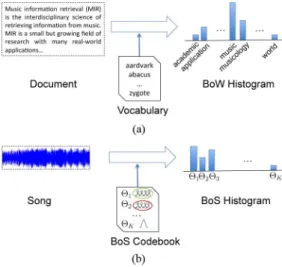
Analogous to the bag-of-words representation of text doc-uments, the BoS approach represents songs with respect to a codebook, where generative models are used in lieu of words. These generative models compactly characterize typical audio features and musical dynamics in songs. A song is then modeled as a composition of these codewords, just as a text document is composed of words, and a BoS histogram is constructed by counting the occurrences of each codeword in the song through probabilistic inference (see Fig. 1).
In this section, we establish a BoS representation for music.
Wefirst discuss the (generative) base models from which we
will derive BoS codewords (Section III-A). We choose Gaussian
Fig. 1. (a) Bag of Words modeling process: a document is represented as a histogram over word counts. (b) Bag of Systems modeling process: a song is represented as a histogram over musical codewords, where each codeword is a generative model that captures timbral and temporal characteristics of music. and dynamic texture (DT) models to capture prototypical tim-bral content and temporal dynamics, respectively, although it should be noted that the BoS representation is not restricted to these choices of generative models. We then present several ap-proaches to learn a dictionary of codewords from a collection of representative songs (Section III-B). Finally, we describe how to map songs to the BoS codebook using probabilistic inference (Section III-C).
A. Generative Models as Codewords
To construct arichcodebook that can model diverse aspects
of musical signals, we consider two different base models, the Gaussian model and the dynamic texture (DT) model [36]. Each captures distinct musical characteristics.
In particular, the audio content of a song isfirst represented by a sequence of audio feature vectors (e.g., MFCCs, which
cap-ture timbre) , extracted from equally spaced,
half-overlapping time windows of length (which determines
the time resolution of the features), where depends on the
duration of the song and the sampling process. Gaussian
code-words will capture average timbral information in unordered
portions of ; DT codewords will model characteristic temporal
dynamics inorderedsubsequences of . Below, we discuss each
base model in more detail. To further increase the diversity of the codebook, we will consider the above base models at dif-ferent time resolutions as well.
1) Gaussian Models: A Gaussian codeword models the
av-erage timbral characteristics of the bag-of-features representa-tion of a sequence of audio feature vectors, without taking into account the actual ordering of audio features. In particular, the model assumes each vector in the bag-of-features is generated
by a multivariate Gaussian , where and are the
mean and the covariance matrix, respectively. Hence the
code-word is parameterized by .
2) Dynamic Texture Models: A dynamic texture (DT)
code-word captures timbre as well as explicit temporal dynamics of an audio fragment (i.e., a sequence of audio feature vectors) by explicitly modeling the sequential ordering of the audio feature vectors.
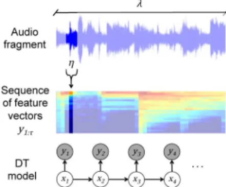
Fig. 2. A dynamic texture model represents a fragment of audio of length . Wefirst compute a sequence of feature vectors, each computed from a window of length . The DT models each feature vector as an observed variable in a linear dynamical system.
Specifically, a DT treats a sequence of audio feature
vectors as the output of a linear dynamical system (LDS): (1) (2)
where the random variable encodes the timbral
con-tent (audio feature vector) at time , and a lower dimensional
hidden variable encodes the dynamics of the
obser-vations over time. The codeword is specified by parameters
, where the state transition matrix
encodes the evolution of the hidden state over
time, is the driving noise process, the
observa-tion matrix encodes the basis functions for
repre-senting the observations , is the mean of the observation
vectors, and is the observation noise. The
ini-tial condition is distributed as . We note that the
columns of the observation matrix can be interpreted as the
principal components (or basis functions) of the audio feature vectors over time. Hence, each audio feature vector can be rep-resented as a linear combination of principal components, with corresponding weights given by the current hidden state. In this way, the DT can be interpreted as a time-varying PCA represen-tation of an audio feature vector time series.
Fig. 2 illustrates the underlying generative process of a DT modeling a sequence of feature vectors. The time scale of a
DT is determined by the duration of an audio-fragment,
and the length of a window from which feature vectors are
computed. Note that the duration is directly determined
by and the number of feature vectors in a sequence, , by
, since we compute feature vectors from half-overlapping windows.
B. Codebook Generation
We are interested in compiling arichcodebook, which effec-tively quantizes the space of music-fragment models. The code-book should have a high representational power for music, i.e., contain a diverse set of codewords that can capture many dif-ferent musical characteristics. First, in order to consider diverse aspects of the musical signal (e.g., timbre in short snippets of audio, or more complex timbral and dynamic patterns in longer
fragments), we choose different base models (i.e., type of
generative model and time scale). We learn the codebook by
learning groups of codewords, where each codeword in a group is derived from a certain base model.
More formally, we define the subset of the codebook
con-sisting of codewords derived from the base model as
, where is the number of codewords derived from
base model . Hence for a given song , the subset of
codewords is associated with a particular feature vector repre-sentation of the song at the specified time scale. For
code-word subset with a Gaussian base model, each codeword
takes the form , and song is
repre-sented as a bag of audio feature vectors ,
extracted from windows of length . For codeword subset
with a DT base model, each codeword takes the form
, and song is represented as a bag
of audio fragments . Audio fragments
are sequences of feature vectors, each feature extracted from
a window of length . The length of an audio fragment is
de-fined as and the step size between successive audio
frag-ments is .
In what follows, we assume that all codeword subsets are the
same size, i.e., . The union
of all these subsets of codewords is the BoS codebook,
, where is the total number of
codewords in the codebook.
In practice, to compile a codebook we select a collection of
representative songs . Then, based on this collection, we
ob-tain some codewords for each of the base models. In
par-ticular, we will learn the codewords in each codeword subset
independently, byfirst generating the corresponding
repre-sentation for each song , and then estimating the
parameters for a set of codewords of that base model to
ade-quately span these audio representations.
A natural approach to this estimation problem is to use the
EM algorithm to directly learn a mixture of codewords (of
base model ) fromallaudio data — i.e., the combined audio
data from all the songs in . However, this becomes expensive
as and the amount of audio data increases. Therefore, we also
investigate alternative methods of codebook generation, which are expected to increase computational efficiency by learning
fewer (than ) codewords at once and/or learning from (small)
subsets of all audio data in .
In particular, we will consider four different procedures for
learning codewords for subset : (1) learneach of the
codewords independently from very small (non-overlapping)
subsets of all available audio data (e.g., from a fragment of a
song in ), (2) learn small mixtures of afew
codewords independently fromsmall(but slightly larger,
non-overlapping) subsets of all available audio data (e.g., from
indi-vidual songs in ), (3) learnall codewords simultaneously
from allavailable audio data in , either by using standard
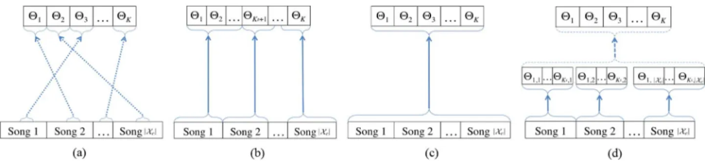
EM, or (4) with recourse to a more efficient,hierarchicalEM (HEM) algorithm. Each of these methods is depicted graphi-cally in Fig. 3. In Section VI-A we experimentally evaluate each codebook generation method, leading us to settle upon the second, song-based method of codebook generation, as the best combination of efficient learning time and good performance.
In what follows, we detail each codebook generation method,
applied to learning a subset of codewords for a single base
Fig. 3. Learning a BoS Codebook by (a) modeling random audio fragments with a single instance of the model, (b) modeling each song with a small mixture model, (c) modeling all available audio data with a large mixture model using standard EM, or (d) using a more efficient, hierarchical EM (HEM) algorithm. A solid arrow corresponds to applying EM, a dashed arrow to applying HEM, and a dotted arrow to direct estimation (see Section III-B.1).
repeat the procedure for each base model and pool the resulting codeword subsets.
1) Fragment-Based Procedure: An individual codeword
is learned directly from a very small subset of all
available audio data in . In particular, to learn a Gaussian
codeword, a song is selected uniformly at random from the
codebook song set , represented appropriately as ,
and a few (sequential) audio feature vectors are (uniformly)
randomly chosen from . The parameters of are then
directly estimated by computing the mean and the (diagonal) covariance matrix of these feature vectors. To learn a DT codeword, again a song is selected uniformly at random
from the codebook song set , represented appropriately as
, and an audio fragment is (uniformly) randomly
chosen from . The parameters of are directly estimated
from the audio fragment, using an approximate and efficient
algorithm based on principal component analysis for DT codewords [36]. The process is repeated until the desired number of codewords ( ) has been collected. With
com-plexity , this is the least computationally expensive
method of codebook generation, as each codeword is learned individually and efficiently from a small amount of data (as shown in Fig. 3(a)). Additionally, since each codeword is learned independently, the learning processes can easily be
parallelized, reducing the complexity to , where
is the number of processors available.
2) Song-Based Procedure: Mixtures of afewcodewords are
learned fromindividual songsin the codebook song set and
are then pooled together to form the codeword set . More
specifically, each song in (represented appropriately as )
is modeled with a Gaussian mixture model (GMM) or dynamic
texture mixture (DTM) model with mixture
components, where the ’s are Gaussian or DT components
and the ’s are the corresponding mixture weights. These
mix-ture models are learned using the EM algorithm (EM-GMM [37] or EM-DTM [38] for Gaussian mixture models or dynamic texture mixture models, respectively). We then aggregate the mixture components (ignoring the mixture weights1) from each
song-level model to form , where .
1The alternative to ignoring mixture weights would be to use the mixture weights when building the BoS histograms for each song — so a more common codeword, with a high mixture weight, is more likely to be assigned to represent a portion of audio than a rare codeword, which would have a low mixture weight. However, it makes more sense assign to a snippet of audio the codeword thatbest
matches, even if it is a rare codeword, to create the most precise representation of the song. In fact, these rare codewords may have more discriminative power than more common codewords, which may occur across many tags.
This approach has a complexity of
, where is the average number of iterations for each
run of the EM algorithm and is the average number of data
samples used as input to the EM algorithm. In the case of
Gaussian codewords, is the average number of audio feature
vectors per song, while in the case of DT codewords, is the
average number of audio fragments per song. In comparison to the fragment-based procedure, the song-based procedure makes use of the entire codebook song set, and provides a regularization effect in learning the codewords by smoothing over an entire song rather than using a single fragment for estimation. As Fig. 3(b) shows, each song is associated with a few codewords, from the corresponding song model. Since song models can be learned in parallel, the complexity can be
reduced to , where again is the number
of processors available.
3) Collection-Based Procedure: All the codewords in
are learned jointly, as one large mixture model, from
all available audio data in the codebook song set . In
particular, for Gaussian codewords, we pool the
bag-of-fea-tures representations of all the songs in , and use this as
input to the EM-GMM algorithm to learn a mixture model
, where each parameterizes a Gaussian and
is the corresponding mixture weight. For DT codewords, we pool the bag-of fragments representations of all the songs
in , and use this as input to the EM-DTM algorithm to
learn a mixture model , where each
param-eterizes a DT and is the corresponding mixture weight.
Each individual mixture component becomes a codeword in (mixture weights are discarded). Therefore, the number
of mixture components corresponds to (the desired number
of codewords in ). The computational complexity of this
procedure is , where
is the number of samples used as input to the EM algorithm.
This approach has a factor of higher time complexity than
the song-based procedure. However, the complexity can be improved by subsampling the inputs to the EM algorithm, i.e.,
using . The EM algorithm usually requires storing
in memory (RAM) all available audio data, and hence scales poorly to large codebook song sets. Even though a parallel implementation of EM could effectively alleviate the high memory requirements (at the likely modest cost of globally coordinating the local computations), the cumulative CPU time requirements would be still elevated because each iteration would still need to process the entire data. Fig. 3(c) shows the collection based procedure.
4) Hierarchical Collection-Based Procedure: Similar to the previous approach, this procedure learns a mixture model with
components from all available audio data in , but now
using a more efficient two-stage procedure. First, a series of mixture models are estimated from small subsets of the data, using EM. Then, after aggregating all mixture components, the resulting (very large) mixture is reduced to a mixture with components using the hierarchical EM algorithm (HEM) [33],
[39]. Specifically, a large collection of codewords of size
is learned from with the song-based procedure, using
mixture components per song. Then, the
codewords in are clustered to form a codeword set of
size using the HEM algorithm for GMMs [39] or
the HEM algorithm for DTMs [33]. In this case, the HEM algo-rithm takes as input a large mixture model
(weighing all mixture components equally), and produces a
reduced mixture model with fewer components ,
where each component is a novel codeword that groups,
i.e., clusters, some of the original codewords. As before, each individual mixture component in the output model becomes a codeword.
The complexity is , where is the
average number of iterations of the HEM algorithm. Assuming
and , this becomes ,
saving a factor compared to the previous, direct
col-lection-based procedure. Furthermore, since learning the song models in thefirst stage can be parallelized, the complexity can
be further reduced to . As before,
is the number of processors available. Fig. 3(d) shows the two stages of this method of codebook generation.
C. Representing Songs With the Codebook
Once a codebook is available, a song is represented by a
BoS histogram , where is the weight of codeword
in the song. To count the number of “occurrences” of a given
codeword in the song, we start from the appropriate
song representation, , at the appropriate time scale. At
var-ious time points in the song (e.g., every seconds), we
com-pare the likelihood of to the likelihood of all other codewords
derived from the same codeword subset, i.e., all (since
likelihoods are only comparable between similar models with
the same time scale). We count an occurrence of at if it
has the highest likelihood of all the codewords in given the
audio data , i.e., . For GMM
codewords, is a single audio feature vector, extracted from a
window of width starting at , while for DTM codewords,
is a sequence of such feature vectors, extracted at intervals
of .
Finally, codeword counts are normalized to frequencies to
obtain the BoS histogram for song :
(3)
We first normalize within each codeword subset — by the
number of fragments, , in — and then between subsets
— by the number of base models, .
Equation (3) is derived from the standard term frequency rep-resentation of a document, where each audio fragment is re-placed by its closest codeword. However, this can become un-stable when a fragment has multiple codewords with (approx-imately) equal likelihoods, which is more likely to happen as the size of the codebook increases. To counteract this effect, we generalize Equation (3) to support the assignment of multiple codewords at each point in the song. We introduce a smoothing
parameter . In particular, we assign the
most likely codewords (within one subset) to each portion of audio. The softened histogram is then constructed as:
(4)
where the additional normalization factor of ensures that
is still a valid multinomial for . The is formally
defined for a function over a discrete set as
such that , and .
IV. MUSICANNOTATION ANDRETRIEVALUSING THE
BAG-OF-SYSTEMSREPRESENTATION
Once a BoS codebook has been generated and songs
repre-sented by BoS histograms, a content-based auto-tagger may be obtained based on this representation — by modeling the char-acteristic codeword patterns in the BoS histograms of songs as-sociated with each tag in a given vocabulary. In this section, we formulate annotation and retrieval as a multiclass multi-label classification of BoS histograms and discuss the algorithms used to learn tag models.
A. Annotation and Retrieval With BoS Histograms
Formally, assume we are given a training dataset , i.e., a
collection of songs annotated with semantic tags from a
vocab-ulary . Each song in is associated with a BoS histogram
which describes the song’s acoustic content with respect to the BoS codebook . The song is also associated with an annotation vector
which expresses the song’s semantic content with respect to ,
where if has been annotated with tag , and
otherwise. In short, a training dataset is a collection of
histogram-annotation pairs .
Given a training set , we estimate a series of tag-level
models that capture the statistical regularities in the BoS
his-tograms representing the subsets of songs in associated with
each tag in , using standard text-mining algorithms. Given
the BoS histogram representation of a novel song, , we can then resort to the previously trained tag-level models to
com-pute the relevance of each tag in to the song. In this work,
we consider two algorithms with a probabilistic interpretation,
which output posterior probabilities that a tag
ap-plies to a song with BoS histogram . We then aggregate the posterior probabilities to form a semantic multinomial (SMN) , characterizing the relevance of each tag to
the song ( and ).
Annotation involves selecting the most representative tags for a new song, and hence reduces to selecting the tags with the highest entries in the SMN . Retrieval consists of rank ordering
to a query. When the query is a single tag from , we define
the relevance of a song to the tag by , and hence retrieval
consists of ranking the songs in the database based on the entry in their SMN.
B. Learning Tag Models From BoS Histograms
The BoS histogram representation of songs is amenable to a variety of annotation and retrieval algorithms. In this work, we investigate one generative algorithm, Codeword Bernoulli Average (CBA), and one discriminative algorithm, multiclass kernel logistic regression (LR).
1) Codeword Bernoulli Average: The CBA model proposed
by Hoffmanet al.[14] is a generative process that models the conditional probability that a tag applies to a song. Hoffman
et al.define CBA based on a vector quantized (VQ) codebook
representation of songs. For our work, we use instead the BoS representation. CBA defines a collection of binary random
vari-ables , which determine whether or not tag
ap-plies to song , with a two-step generative process. First, a
code-word is chosen according to the distribution
given by the song’s BoS histogram , i.e.,
(5)
Then, a value for is chosen from a Bernoulli distribution
with parameter , which represents the probability of tag word
given codeword :
(6)
We use the author’s code [14] to fit the CBA model, i.e.,
learn the parameters . To obtain the SMN of a novel song with BoS histogram , we compute the posterior probabilities under the estimated CBA model, and
nor-malize by its norm.
2) Multiclass Logistic Regression: For each tag, logistic
re-gression defines a linear classifier with a probabilistic interpre-tation byfitting a logistic function to BoS histograms associated and not associated with the tag:
(7) Kernel logistic regression [40]finds a linear classifier after
applying a non-linear transformation to the data, .
The feature map is indirectly defined via a kernel function
.
In our experiments, we use the histogram intersection kernel [41], which is defined by the kernel function:
(8)
where and are BoS histograms. In our implementation we
use the software package Liblinear [42] to learn an
-regular-ized logistic regression model for each tag using the “one-vs-the rest” approach. We select the regularization parameter by per-forming 4-fold cross-validation on the training set. Given the BoS histogram of a new song , we collect the posterior
prob-abilities and normalize to obtain the song’s SMN.
V. MUSICDATA
In this section we introduce the two music datasets used in our experiments, along with the audio features and the base models used for the codewords.
A. CAL500 Dataset
The CAL500 [5] dataset consists of 502 Western popular songs from 502 different artists. Each song-tag association has been evaluated by at least 3 humans, using a vocabulary of 149 tags, including genres, instruments, vocal characteristics, emo-tions, acoustic characteristics, and use cases. CAL500 provides binary annotations that can be safely considered as hard labels,
i.e., when a tag applies to the song and 0 when the
tag does not apply. We restrict our experiments to the 97 tags with at least 30 example songs. CAL500 experiments use 5-fold cross-validation where each song appears in the test set exactly once.
B. CAL10K Dataset
The CAL10K dataset [43] is a collection of over ten thousand songs from 4,597 different artists, weakly labeled (i.e., song an-notations may be incomplete) from a vocabulary of over 500 tags. The song-tag associations are mined from Pandora’s web-site. We restrict our experiments to the 55 tags in common with CAL500.
C. Codeword Base Models and Audio Features
We choose a priorifive different base models for codewords:
two time scales of Gaussians ( and ) and three time scales
of DTs ( , and ). These time scales were chosen by
referring to previous work [5], [6], and with the goal of spanning a reasonable range of scales that occur in music. For example,
codewords from model class will capture dynamics that
unfold over a few milliseconds to while codewords from model
class will capture dynamics that unfold in the time span of
several seconds. We will experimentally determine the best base
models and combinations of models from these five choices.
For the Gaussian codewords, we use as audio features thefirst 13 Mel-frequency cepstral coefficients (MFCCs) appended with
first and second instantaneous derivatives (MFCC deltas). This results in 39-dimensional feature vectors [44]. For the DT
code-words, we model 34-bin Mel-frequency spectral features.2We
note that these features represent timbre, but not other facets of music such as rhythm or tonality.
To motivate the difference in features between Gaussian and
DT codewords, note that Mel-frequency cepstral coefficients
(MFCCs) use the discrete cosine transform (DCT) to decorre-late the bins of a Mel-frequency spectrum. In Section III-A.2 we noted that the DT model can be viewed as a time-varying PCA representation of the audio feature vectors. This suggests that we can represent the Mel-frequency spectrum over time as the output of the DT model. In this case, the columns of the ob-servation matrix (a learned PCA matrix) are analogous to the DCT basis functions, and the hidden states are the coefficients (analogous to the MFCCs). The advantage of learning the PCA representation, rather than using the standard DCT basis, is that 2We use 30 Mel-frequency bins to compute the MFCC features, which pro-vides a similar spectral resolution to the 34-bin Mel-frequency features.
TABLE I
DESCRIPTION OFBASEMODELSUSED INEXPERIMENTS: TWOTIMESCALES OFGAUSSIANS ANDTHREETIMESCALES OFDTS
different basis functions (matrices) can be learned to best repre-sent the particular codeword, and different codewords can focus on different frequency structures. Also, note that since the DT explicitly models the temporal evolution of the audio features, we do not need to include their instantaneous derivatives (as in the MFCC deltas).
In both cases, feature vectors are extracted from half-over-lapping windows of audio. The window and fragment length for each codeword base model are specified in Table I. These choices were intended to cover a few sufficiently distinct time resolutions, and the step size between fragments is relatively small in order to increase the number of fragments we can ex-tract from each song.
VI. EXPERIMENTALEVALUATION
In this section we present experimental results on music an-notation and retrieval using the BoS representation. Annota-tion performance is measured using mean per-tag precision (P), mean tag recall (R) and mean tag F-score. Retrieval per-formance is measured using area under the receiver operating characteristic curve (AROC), mean average precision (MAP), and precision at 10 (P10) averaged over all one-tag queries. We refer the reader to Turnbullet al.[5] for a detailed definition of these metrics.
A. Design Choices
The combination of four codebook generation methods,five
base models of codewords and two BoS histogram annotation algorithms creates a large number of possibilities for the im-plementation of the BoS framework. Along with the choice of
codebook size and histogram smoothing parameter , it
be-comes difficult to present an exhaustive comparison of all pos-sibilities. We instead evaluate each design parameter indepen-dently while keeping all other parametersfixed, which leads us to select (1) the song-based procedure for codebook generation,
(2) a combination of three codeword base models ( , ,
and ; see Table I), and (3) logistic regression to annotate BoS histograms. Appendix I discusses each of these design choices in more detail. For each design choice, alternatives are com-pared by measuring the annotation and retrieval performance of a series of BoS auto-taggers. In the experiments in this sec-tion, reported metrics are the result offive-fold cross-valida-tion where tag model training and testing are done using LR on CAL500.
1) EXP-1: Codebook Generation Methods: Wefirst
com-pare the four methods of codebook generation presented in Section III-B. We restrict our attention to codebooks consisting
TABLE II
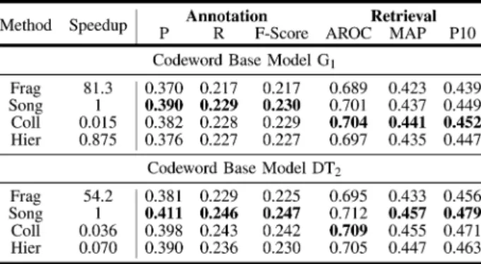
EXP-1: LEARNING ABOS CODEBOOKWITHFOURDIFFERENTMETHODS: FRAGMENT-BASED(FRAG), SONG-BASED(SONG) COLLECTION-BASED
(COLL)ANDHIERARCHICAL(HIER). CODEWORDS ARELEARNED
FROM ACODEBOOKSONG SET OF SONGS. BOS HISTOGRAMS USE
SMOOTHINGPARAMETER ,AND AREANNOTATEDWITHLR.
SPEEDUP ISREPORTEDRELATIVE TO THESONG-BASEDMETHOD
of a single base model ( only or only) and use a small
codebook size (because for the collection-based codebook
learning procedures, learning time quickly becomes prohibitive with larger values of ). Additional parameter settings for this experiment can be found in Appendix I.
Annotation and retrieval results for these experiments are
reported in Table II. We find that learning codewords with
the song-based procedure produces the best combination of performance and efficiency. While highly efficient, learning codewords at the fragment level gives sub-optimal perfor-mance. The collection-based procedure (with standard EM) provides good performance in terms of annotation and retrieval, but training times are an order of magnitude higher than the song-based method. Moreover, the results in Table II are for
relatively small codebooks — as the codebook size
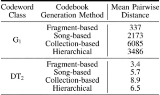
increases, the computational cost of the EM algorithm becomes even more prohibitive. In Appendix I we analyze the code-books produced by each method in more detail, in particular investigating the diversity and spread of the learned codewords using appropriate pairwise distances and 2-D visualization. Hence, for the remainder of experiments codebooks are learned by the song-based method.
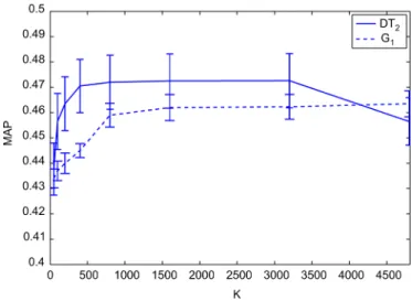
2) EXP-2: Codebook Size: In this experiment we investigate
the effect of the codebook size, , on annotation and retrieval performance. Fig. 4 plots the retrieval performance (MAP) as
a function of the codebook size, for values of ranging from
50 to 4800. Further details about the parameter settings for this
experiment are provided in Appendix I. Wefind that once the
codebook has reached a certain size, adding more codewords has a negligible effect on performance, and in fact for DT code-words performance eventually degrades as the codebook
be-comes large. We see an optimal range for between 800 and
3200, corresponding to an optimal range for between 2 and
8. Based on these results we choose for future experiments
(corresponding to ) for each codeword group, for
codebooks learned from CAL500. We note however, that these results are for a single base model, and we see in preliminary ex-periments that when codewords from a variety of different base models are combined, we can use a larger codebook without sat-urating performance (see Section VI-A). We also note that these
Fig. 4. EXP-2: Retrieval performance (MAP) as a function of BoS codebook size . Each codebook is generated with a song-based approach. For afixed codebook song set , the codebook size is varied by varying the number of codewords learned per song, . The error bars indicate the standard error over thefive cross-validation folds of CAL500.
TABLE III
EXP-3: RESULTSUSINGBOS CODEBOOKSWITHCODEWORDSFROMVARIOUS
BASEMODELS. ALLCODEBOOKSHAVE CODEWORDS, WITH
VARYINGNUMBER OFCODEWORDBASEMODELS, , CODEWORDS PER
BASEMODEL, ,ANDSIZE OFSONGMODEL, . BOS HISTOGRAMS USE
SMOOTHINGPARAMETER ,AND AREANNOTATEDUSINGLR
We found in preliminary experiments that with a larger
code-book song set, we can keep in a similar range, allowing for
larger codebooks before performance deteriorates. In particular, when using the CAL10K dataset as the codebook song set, we
set (see Section VI-B.2).
3) EXP-3: Codeword Base Models: One of the key
advan-tages of the BoS framework is that it allows one to leverage codewords from different base models (i.e., model types and time scales) to produce a rich codebook. In this set of experi-ments, we investigate the extent to which using multiple base models is useful.
We evaluate various combinations of the codeword base models defined in Table I, adjusting the number of codewords
learned from each base model, , to obtain afixed codebook
size . We begin with a codebook with all codewords of
base model , which was the best performing individual
codeword base model in preliminary experiments, and com-pare it with codebooks containing additional base models of codewords. Additional parameter settings can be found in Appendix I.
Results are presented in Table III. Wefind that using multiple types of generative models with different time scales in a
code-book is beneficial. Compared to a codebook of codewords
only, adding Gaussian codewords3(i.e., ) or DT codewords
on a shorter time scale4(i.e., ) leads to a significant im-provement in performance. In particular, the best performance is achieved when all of the above base models are combined:
, and . This is a significant improvement in
per-formance over the , codebook.5 While Fig. 4 shows
that adding more codewords of thesamebase model to a
code-book of size 1600 saturates and eventually deteriorates perfor-mance, Table III illustrates that adding codewords of adifferent
base modelcan further improve performance. This confirms the
codebook isenrichedwith codewords that model different
as-pects of the musical signal.
We notice, however, that adding a third set of DT codewords no longer improves performance. We speculate this is because
the and base models use feature vectors sampled at
the same time resolution, ; they differ in the number of feature vectors, , in the fragments they model, which is twice as long
for as . The hidden state of a DT model evolves as a
first order Markov process, with the evolution from state to defined by the transition matrix . While a different time resolution can significantly affect , the model (and the corre-sponding codewords) does not explicitly encode the fragment length, . The latter only defines the length of the input audio fragments used in the learning stage of the algorithm. Using larger values of means using longer audio fragments, resulting
in more smoothed DT models. Hence the codewords in and
may capture more or less the same dynamics, although the
codewords in may be more smoothed than those in .6
Similarly, adding a second set of Gaussian codewords pro-vides no improvement in performance. Indeed, since Gaussians do not model temporal dynamics, the only time scale parameter to tune is the window length (i.e., ), varying which determines the amount of audio that is averaged over to produce timbral features. Therefore, features extracted at the time scale for are essentially more smoothed versions of the features extracted
for (with slightly different frequency bands), and the
code-words capture much of the same timbral information.
4) EXP-4: BoS Histogram Smoothing Parameter : In this
experiment we investigate the effect of the BoS histogram
smoothing parameter on annotation and retrieval
perfor-mance. Fig. 5 illustrates a few example BoS histograms with
varying values for for a song from CAL500. When building
BoS histograms, we assign the most likely codewords (of
each base model) to each portion of audio. Hence when a smaller value of is used, songs tend to be represented by only a few different codewords, leading to more peaked histograms, while a larger value of creates smoother histograms.
Details of the experimental setup are provided in Appendix I. Results are plotted in Fig. 6 as a function of . Wefind that the performance is fairly stable for a wide range of values for ,
reaching a peak between and . The performance
drops off gradually for large and more steeply for small .
This leads us to select as the BoS histogram smoothing
parameter for further experiments. 3Paired t-test of MAP score on 97 tags: 4Paired t-test of MAP score on 97 tags: 5Paired t-test of MAP scores on 97 tags: 6See Chan and Vasconcelos [38] for more details.
Fig. 5. BoS histograms with smoothing parameter , 10 and 50 for Guns N’ Roses’November Rain. The smoothing parameter determines the number of codewords to be assigned at each point in the song, so using a smaller value of will assign only a few different codewords, leading to more peaked his-tograms, while a larger value of creates smoother histograms. Note the dif-ferent y-axis scales.
Fig. 6. EXP-4: Annotation (F-score) and retrieval (MAP) performance of the BoS approach, using LR on the CAL500 dataset, as a function of the smoothing parameter .
We also notice throughout these (and following) experiments that LR tends to outperform CBA as an annotation algorithm, and hence LR is our annotation algorithm of choice.
B. BoS Performance
In this section we present experiments that demonstrate the effectiveness of the BoS representation for music annotation and retrieval, using the design choices made in the previous sec-tion. We compare the BoS approach to several baseline autotag-gers on the CAL500 and CAL10K datasets.
1) Results on CAL500: We run annotation and retrieval
ex-periments on CAL500 using two BoS auto-taggers based on a
codebook of size which combines codeword base
models , and , each with and obtained
with the song-based method and
his-togram smoothing parameter . One auto-tagger uses
LR to annotate BoS histograms and the second uses CBA — BoS-LR and BoS-CBA, respectively. For LR, the regularization parameter is chosen by 4-fold cross-validation on the training set. All reported metrics are the result offive-fold cross-valida-tion, where for each split of the data the whole training set is
used as the codebook song set (i.e., ).
We compare our BoS-CBA and BoS-LR auto-taggers with three state-of-the-art baselines for automatic music
tagging. The first two are based on hierarchically trained
GMMs (HEM-GMM) [5] and hierarchically trained DTMs (HEM-DTM) [6], respectively. Note that the HEM-GMM and
TABLE IV
BOS CODEBOOKPERFORMANCE ONCAL500, USINGCBAANDLR,
COMPARED TOGAUSSIAN TAGMODELING(HEM-GMM), DTMTAG
MODELING(HEM-DTM), AVERAGING OFGMMANDDTMTAG
MODELS(HEM-AVG)ANDVQ CODEBOOKSWITHLR
HEM-DTM approaches each leverage one base model from among those selected for our BoS codewords, but use it to directly represent tag-specific distributions on low-level audio feature spaces. In particular, the HEM-GMM auto-tagger learns
tag-level GMM distributions with mixture components
over the same audio feature space as . The HEM-DTMfits
tag-level DTM distributions with mixture components
over the same space of audio fragments as used for . The
hyperparameters for these methods were set to those used in previous works [5], [6].
The third baseline, HEM-AVG, averages (on a tag-by-tag basis, by directly averaging the SMNs) the predictions of three HEM auto-taggers: two versions of HEM-DTM (based on
and , respectively) and HEM-GMM (based on ).
The fourth baseline (VQ-LR) is based on a VQ representa-tion of songs [18]. Each song is represented as a Bag-of-Words (BoW) histogram by vector-quantizing its MFCC features with
a VQ codebook of size , and annotation is
imple-mented using -regularized logistic regression. In preliminary
experiments we found that, similarly to the BoS representa-tion, using a softened BoW histogram results in superior per-formance, and consequently we used a smoothing parameter of to build VQ histograms. These hyperparameters were tuned using cross-validation over the CAL500 dataset, using the same methodology as for the BoS hyperparameters.
Results for these experiments are reported in Table IV. The BoS auto-taggers based on LR and CBA outperform the other approaches on all metrics except precision, where HEM-DTM performs best. HEM-AVG outperforms HEM-DTM and HEM-GMM in retrieval metrics, indicating that leveraging multiple time scales and models is beneficial in general, but BoS outperforms HEM-AVG, which demonstrates the addi-tional modeling power the BoS framework provides.
In addition, we also notice that tagging BoS histograms with LR leads to higher performance than CBA. This is not sur-prising, as LR is a discriminative algorithm which is typically better suited when training on small, hard-labeled datasets such as CAL500, whereas CBA is a generative algorithm.
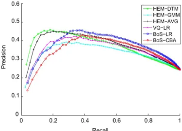
We plot precision-recall curves for each of these auto-taggers in Fig. 7. First, we notice that BoS-LR achieves the best pre-cision-recall trade-off point, and has the best precision for in-termediate and large values of recall. However, at low levels of recall, HEM-DTM has the highest precision — meaning some DTM tag models may befinely tuned to capture certain patterns associated with a tag, at the risk of not generalizing to all oc-currences of that tag. We also note that BoS-LR has a higher precision than BoS-CBA at all levels of recall.
Fig. 7. Precision-recall curves for various auto-taggers on CAL500. HEM-DTM dominates at low recall, but BoS outperforms HEM-DTM at higher recall.
TABLE V
TOP-10 RETRIEVEDSONGS FOR“FEMALELEADVOCALS”. SONGSWITH
FEMALELEADVOCALS AREMARKED INBOLD
In order to provide a qualitative sense of how the BoS auto-tagger performs for retrieval, Table V shows the top-10 retrieval results for the query “female lead vocals”, for the three autotag-gers HEM-GMM, HEM-DTM and BoS-LR.
2) Results on CAL10K: In order to analyze the performance
of the BoS approach when dealing with larger, weakly labeled music collections, which are more representative of web-scale applications, we train both the codebook and the annotation
models on CAL10K. Specifically, we subsample from CAL10K
a codebook song set consisting of one song from each artist
TABLE VI
BOS CODEBOOKPERFORMANCE FORTRAINING TAGMODELS ONCAL10KAND
EVALUATING ONCAL500, USINGCBAANDLR, COMPARED TOGAUSSIAN
TAGMODELING(HEM-GMM), DTMTAGMODELING(HEM-DTM),
ANDVQ CODEBOOKSWITHLR
(i.e., ), and use the song-based method with
to compile a BoS codebook, resulting in
code-words from each base model. (Because the codebook song set is much larger in this experiment than in previous CAL500 exper-iments, wefind that it can support much larger codebook sizes.) Similar to the CAL500 experiments, we use three base models
of codewords, , and , leading to
codewords overall. As CAL10K is not well suited for evaluation purposes, (due to the weakly labeled nature of its annotations the absence of a tag in a song’s annotations does not generally imply that it does not apply to the song), we train BoS tag models on all of CAL10K, and reliably evaluate them on CAL500. Our experiments are limited to the 55 tags that
CAL10K and CAL500 have in common. Wefix the
hyperpa-rameters to the best setting found through cross-validation on CAL500 (see Section VI-B.1), i.e., BoS histogram smoothing
parameter and LR regularization trade-off . We
compare the performance of BoS codebooks to the HEM-GMM, HEM-DTM, and VQ-LR autotaggers.
Annotation and retrieval results reported in Table VI demon-strate that the BoS approach outperforms direct tag modeling also using larger, weakly annotated collections for training. In addition, we notice that BoS-CBA catches up with BoS-LR on several performance metrics. This is a consequence of the weakly-annotated nature of CAL10K, which makes the employ-ment of generative models (such as CBA) more appealing rela-tive to discriminarela-tive models (such as LR).
VII. DISCUSSION
In this section we look at the performance of the BoS au-totagger in more detail, substantiating the claims we made in the introduction about the advantages of the BoS framework. Namely, that decoupling modeling music from modeling tags makes the BoS system more robust for tags with few training ex-amples (Section VII-A), that combining multiple types and time scales of generative models improves performance (VII-B) and that incorporating unlabeled songs when building a codebook is advantageous (VII-C).
A. Decoupling Modeling Music From Modeling Tags
As anticipated in the introduction, we expect that the BoS approach will be particularly robust for tags with fewer training examples when compared to traditional generative algorithms, because the relatively simpler tag models used in the BoS ap-proach are less prone to overfitting. To demonstrate this, we an-alyze performance on subsets of CAL500 tags defined by their
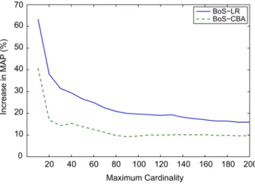
Fig. 8. Retrieval performance (MAP) of the BoS approach, relative to HEM-DTM, as a function of maximum tag cardinality. For each point in the graph, the set of all CAL500 tags is restricted to those associated with a number of songs that is at most the abscissa value. Experiments are run on the resulting (reduced) data set as described in Section VI-B.1, and the performance metrics are averaged over each tag subset.
the cardinality of a tag is defined as the number of
exam-ples in the data set that are labeled with the tag.
We report retrieval performance for both the BoS ap-proaches and the direct generative approach with DTM models (HEM-DTM), using the experimental setup in Section VI-B.1. In Fig. 8 we plot the relative improvement in retrieval perfor-mance (MAP score relative to the MAP score of HEM-DTM) for both BoS auto-taggers as a function of maximum tag car-dinality. The BoS approach achieves the greatest improvement for tags with few training examples. Since the BoS approach decouples modeling music from modeling tags, simple tag models (with few tunable parameters) can leverage the full descriptive power of a rich BoS codebook while avoiding the risk of over-fitting small training sets.
B. Combining Codeword Base Models
A key advantage of the BoS framework is that it enables com-bining different types of generative models over various time scales in a single auto-tagger. We expect that different tags will be better modeled by different model types and time scales. Covielloet al.discuss this in [6], noting that DTM models are more suitable for tags with characteristic temporal dynamics (e.g., tempo, rhythm, etc.)), while some other tags are well char-acterized by timbre alone and thus are better suited for GMMs. A framework such as BoS, which allows the combination of model types and time scales, can therefore enable good per-formance over these different kinds of tags by learning to use codewords from the most suitable base model class in each tag model.
To illustrate this, Table VII compares the annotation (F-score) performance of a BoS-LR autotagger based on four codebooks,
using: (1) base model only (2) base model only (3)
base model only, and (4) base models , and ,
for a few tags in the CAL500 dataset.
DT codewords prove suitable for tags with significant tem-poral structure, such as vocal characteristics and emotions such as “angry” and “aggressive”. Instruments such as electric guitar
TABLE VII
COMPARISON OFPER-TAGF-SCORES FORBOS AUTOTAGGERSBASED ONFOUR
CODEBOOKS: (1) BASEMODEL ONLY(2) BASEMODEL ONLY(3)
BASEMODEL ONLY AND(4) BASEMODELS , AND
and synthesizer also perform well, perhaps because these in-struments exhibit some temporal signature that is captured in the model. We can infer that tags that perform better with are characterized by dynamics that unfold more quickly than tags that perform better with , e.g., “fast” (recall that models fragments of 726 ms, at a resolution of 12 ms per
fea-ture vector, while models fragments of 5.8 s, at a resolution
of 93 ms per feature vector). Additionally, as the performance
averaged over all the tags is a bit higher with codewords,
we gather that the longer time scale is a better “catch-all” to model a wide range of tags. Other tags, such as “low energy” and “mellow” seem to have little in the way temporal dynamics to model, and are best described by timbre information alone.
We note that the BoS codebook combining all three base models often leads to comparable or higher performance to the highest performing individual base model codebook.
C. Incorporating Unlabeled Songs in the Codebook Song Set
An additional advantage of the BoS framework is that the codebook can be learned without an annotated corpus of audio data. This suggests that the codebook can be enriched by expanding the codebook song set to include potentially large, unannotated music collections. To illustrate this intuition, we compare a variety of BoS auto-taggers, each of which differ in
the codebook song set .
We start by forming three different codebook song sets by
aggregating subsets of CAL10K and CAL500: (1) ,
the codebook song set corresponding to the training set for each cross-validation split of CAL500 (as in Section VI-B.1), (2) , a codebook song set that is a subset of 400 ran-domly selected songs from the CAL10K collection and (3)
, the codebook song set that is a subset of the CAL10K dataset consisting of one song from each of the 4,597 artists (as in Section VI-B.2). Note that, since we are using only
TABLE VIII
BOS CODEBOOKPERFORMANCE ONCAL500 USINGCODEBOOKSLEARNED
FROMVARIOUSCODEBOOKSONGSETS. BOS HISTOGRAMS USESMOOTHING
PARAMETER AND AREANNOTATEDWITHLR
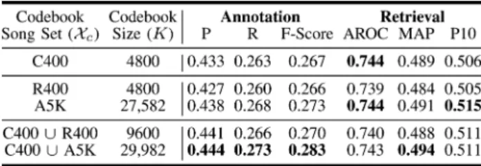
dataset, and thus R400 and A5K, can be considered as collec-tions of unlabeled data that could be used to form a codebook song set. In addition, we consider codebooks derived from the union of C400 with R400 and A5K, respectively. This is a prac-tical scenario — an annotated music collection is augmented with additional unlabeled songs to build a richer codebook.
Details of the experimental setup can be found in Appendix III. Annotation and retrieval results are reported in Table VIII. We notice that the best performances are ob-tained when a richer codebook is produced from combining the training set (i.e., C400) with a much larger collection of
unlabeled music, corresponding to in Table VIII.
Adding only a small set of unlabeled music to the codebook
song set (i.e., ) does not lead to substantial
improvements over using only the training set.
We have shown before (in Section VI-A) that as we learn in-creasingly more codewords from the same collection, perfor-manceflattens and then deteriorates. However, if we increase the size of our codebook song set, the added information allows us to extract larger codebooks that are effectively enriched. This results in a slight improvement of performance.
In addition, we notice that when codebook song sets are equally sized, using the training collection as the codebook song set (C400) outperforms using a different collection (R400). This result may be affected by the fact that CAL500 is mostly pop music, while CAL10K has many other genres (classical, jazz, etc.), so codewords learned from CAL10K may not be as relevant for CAL500. However, growing the size of the collec-tion of unlabeled songs (A5K) allows it to catch up with, and in fact outperform, the C400 codebooks. The ability to leverage a large codebook compiled off-line could, for example, be useful for an application that learns personalized retrieval models. Such a system should be based on a BoS codebook large and varied enough to represent well the music various users are interested in. Personalized tag models can then be learned from a smaller, user-specific collection, perhaps located on the user’s personal device. As demonstrated in Section VI-B.1, these simple tag models can be estimated reliably even when the collection of songs associated with a specific tag is relatively small, as might be the case when training on a user’s personal collection of music.
VIII. CONCLUSION
We have presented a semantic auto-tagging system for music that leverages a rich “bag of systems” representation based on generative modeling. The BoS representation allows for the integration of the descriptive qualities of various generative
models of musical content with different time resolutions into a single histogram descriptor of a song. This approach improves performance over traditional generative modeling approaches to auto-tagging, which directly model tags using a single type of generative model. It also proves significantly more robust for tags with few training examples, and can be learned from a representative collection of songs which need not be annotated. We have shown the BoS representation to be effective for training annotation models on two very different datasets, one small and strongly annotated and one larger and weakly annotated, demonstrating its robustness under different scenarios.
APPENDIXA
DETAILS OFDESIGNCHOICESEXPERIMENTS
This Appendix provides the details of the parameter settings and design for the experiments in Section VI-A.
EXP-1: Codebook Generation Methods: In this
experi-ment we learn codebooks using each of the four methods of codebook generation presented in Section III-B.
For each codebook generation method and each cross-valida-tion split of CAL500, we construct one codebook based on
only and a second codebook based on only. We learn
code-books of size (We choose small because for the
collection-based codebook learning procedures, learning time quickly becomes prohibitive with larger values of ). We select
a small (in order to keep small with ) random subset
of songs from the training set of CAL500 to form a codebook
song set of size . For the fragment-based method,
each codeword is directly estimated from a randomly selected subset of audio data, consisting of 100 (sequential) feature
vec-tors for Gaussian codewords and a fragment of feature
vectors for DT codewords. For the song-based method we set , and for the hierarchical collection-based method we
set . For the collection-based method we subsample the
input data to alleviate the high cost in computational time of the EM algorithm. For the Gaussian codebook we randomly sub-sample 250,000 input feature vectors and for the DT codebook
we randomly subsample 5000 input fragments ( of the
data in both cases).
We build BoS histograms with smoothing parameter and use LR for annotation and retrieval. Tag model training and testing are done on CAL500, usingfive-fold cross-validation.
EXP-2: Codebook Size: In this experiment we investigate
the effect of the codebook size, , on annotation and retrieval performance. For each cross-validation split of CAL500, we use the song-based method to compile codebooks using the training
set as the codebook song set (Now that we have settled
on the song-based method of codebook generation, we can effi -ciently build larger codebooks from a larger codebook song set).
We learn one codebook from base model and a separate
codebook from base model . We vary the size of the
code-book, , from 50 to 4800 codewords. As the number of songs
in the codebook song set isfixed7, i.e., , we vary the
codebook size by changing , i.e., the number
of codewords learned per song. When learning codebooks con-sisting of fewer than 400 codewords, we group multiple songs to 7Actual sizes of thefive training splits are either 401 or 402 songs, we sub-sample to 400.