Abstract
This article presents one solution to the parameterization problem for automated road feature extraction models. Using a line-length buffer approach, a measure of agreement be-tween extracted road features and reference road features is defined. An automated approach for deriving this agreement index is presented and implemented as a parameterization model. Coupling the implemented parameterization model with an existing transportation feature extraction model is demonstrated. Although the solution was designed for a road feature extraction model (FEM), the conceptual design could be applied to other linear FEMs, such as models for streams, fault lines, and isolines.
Introduction
Calibration of the parameters in a road feature extraction model is typically performed through an iterative staged ap-proach using visual comparisons. The stagesin this visual ap-proach are (1) setting of the model parameters, (2) extraction of features from the model run, (3) visual comparison of re-sults to a reference set, and (4) a repeat of the first three stages numerous times. The “best” parameterized model is con-cluded when the agreement (or accuracy) between model re-sults and reference data is maximized. Visible comparisons are favored because of the endemic mis-registration problems and line-to-line correspondence problems plaguing an auto-mated approach. A sparse sampling of the parameter space has been favored because of the combinatorial problems of multiple parameters and the limitation of human efficiency for evaluating model results by visual analysis.
Although automated methods for parameterizing road fea-ture extraction models have been argued (Wang, et al., 1992), little research has focused on this issue. Conceptual and im-plementation impediments have prevented automated ap-proaches for comparing the model results and reference linear features. An automated solution to the parameterizationof road feature extraction models would enable a broad sensitiv-ityanalyses to be conducted using multiple parameters and range in values. For instance, how well the feature extraction model performs in other geographic areas, image types, and spatial resolution is of interest. As most road feature extrac-tion models are evoluextrac-tionary (i.e., under continual refine-ment), such an automated solution would also enable efficient assessments of each model refinement.
A Parameterization Model for
Transportation Feature Extraction
Michael E. Hodgson, Xingong Li, and Yang Cheng
Automated approaches for parameterizing such models or conducting sensitivity analyses would obviously require an automatedmethod for evaluating model performance (i.e., an accuracy assessment). This article presents one solution to the problem of an automated parameterization of road feature ex-traction models. This research builds on work in assessing spatial accuracy of linear features by Goodchild and Hunter (1997) using a line-length buffered approach. However, in the current research the assumptions and unknowns of Goodchild and Hunters’ buffered line method for accuracy assessment are inverted.
In this article, the conceptual nature of the accuracy as-sessment problem is first presented. Next, the proposed line-length buffered theme approach is presented along with the measure of agreement. The parameterization model was imple-mented in an embedded GIS approach and demonstrated using the road feature extraction model (FEM) from the Oak Ridge National Laboratory (ORNL). The algorithmic logic behind the ORNL FEMis briefly presented.
Parameterization and Accuracy Assessment Problem
Approaches for extracting transportation features from re-motely sensed imagery may be categorized into autonomous methods and interactive (i.e., semi-autonomous) methods. In-teractive methods, typically more successful, are guided by human operators that “train” the algorithms spectrally, spa-tially, or topologically. In some implementations, the interac-tive methods require frequent nudges and guidance for many features in an image. The parameters in interactive methods may be continually changed. Autonomous methods require no user input once they are parameterized. Autonomous meth-ods, however, require careful prior parameterization for the geographic area and specific imagery.Parameterizing a model is performed by conducting accu-racy assessments on the output of different parameter combi-nations. The conceptual goal in the accuracy assessment is to compare one extracted feature to one reference feature (or set of extracted features to a set of reference features) and assess the level of “agreement” between features. If the reference fea-ture is considered “truth” the analysis is an accuracy assess-ment, otherwise it is considered a measure of agreement. This distinction is important for those studies focused on change-detection or a better representation of the transportation fea-tures, as in versioning. This study assumes the transportation reference features are “truth.”
In the context of transportation feature extraction models, the three logical choices for conducting an accuracy assess-ment would be a: (1) visual comparison, (2) automated Michael E. Hodgson is with the Department of Geography,
University of South Carolina, Columbia, SC 29208 ([email protected]).
Xingong Li is with the Department of Geography, University of Kansas. Lawrence, KS 66045.
Yang Cheng is with the Machine Vision Group, Jet Propulsion Laboratory, Pasadena, CA 91109.
Photogrammetric Engineering & Remote Sensing Vol. 70, No. 12, December 2004, pp. 1399–1404. 0099-1112/04/7012–1399/$3.00/0 © 2004 American Society for Photogrammetry and Remote Sensing
comparison (in a raster model), or (3) automated comparison (in a vector model).
Visual accuracy assessments suffer from the same prob-lem of quantitatively measuring success as do digital ap-proaches; for example, determining which of the following characteristics define correctness:
•
geometry (e.g., length of feature, number of nodes in feature curvature)•
number of distinct segments (e.g., road composed of n-segments with intersections)•
continuity (i.e., no gaps)•
spatial accuracy (i.e., deviation of extracted feature from refer-ence feature)•
commission errors (i.e., incorrectly identified road segments).The following example questions further elaborate on these issues. Is the correct identification of a 100 meter road segment considered equally important as the correct identifi-cation of a 1600 meter road segment? If the reference road is represented by two extracted segments with a small gap, is this considered a success, partial failure, or failure? If the ref-erence feature is defined from a different scale (i.e., spatial res-olution) of imagery than the imagery used for automated fea-ture extraction, how should commensurate spatial differences in geometry and spatial accuracy be considered? Are these geometric or spatial differences caused by scale-considered failures? If more than one of the measures above are used are the measurements weighted equally? There is no agreement on above measures of success, particularly, the last question on weightingeach measure.
A visualcomparison between the model results and the reference data is the common approach used in parameteriz-ing any extraction model. First, parameter settparameteriz-ings are set, and the model is run. The output road features are visually com-pared to the reference source. Based on the results, a new set of parameter values is set, and the process is repeated. Such an approach is commonly used in selecting training sites for supervised classification procedures. The visual comparison is appropriate as a guide to parameterization if: (1) the num-ber of parameters is relatively small, and (2) the “accuracy” of the extracted features can be adequately assessed. The sheer number of iterations involved with a large set of parameters, many of which are co-dependent, would prohibit the visual approach. Yet, the visual approach clearly dominates research in transportation feature extraction as alternatives are less de-sirable. Thus, the evaluation of model sensitivity to imagery and geography or the evaluation of a large range/combination in parameter values is compromised.
A digital comparison of the transportation pixels identi-fied in the image and the reference transportation pixels would solve the computational problem associated with the number of parameters. This approach may be implemented as a map overlay in a rasterdata model. As in the visual approach, the iterative method of setting parameter values, comparison of ex-tracted and reference features, and resetting parameters for a new run, is still followed. However, as with all pixel-to-pixel comparisons, it assumes the two maps are in perfect, spatial registration. In most real-world applications this spatial agree-ment is seldom true. Assessing accuracy of linear features using a raster approach is thus, seldom performed.
A digital comparison of extracted roads to reference roads in vectorform is generally the ideal, as extracted roads typi-cally populate a database in a vector model form. However, because the precision in representing the spatial location of critical points is so great, a comparison of vector themes using the critical points in corresponding lines will suggest nearly total disagreement. Coincident-paired points in the reference and FEMextracted line will rarely occur. One coverage may be more generalized than another, resulting in a different number of points for the reference line than the extracted line.
Some related work in feature extraction using “snakes” (Agouris, et al., 2001) is based on matching extracted features to pre-existing reference features using energy measures: spac-ing of nodes, curvature, and local gradient. It is possible that this approach could be used as the assessment approach within a parameterization model. The implicit assumption and resulting problem for applying these snake measures to a holistic accuracy assessment of multiplefeatures is that each pairof reference road and extracted road must be compared in isolation from all other reference roads and extracted objects. In other words, the specific road portion to “match” to must be known. Problems may occur if the FEMroad segment is in-complete. Issues of scale differences may also complicate an autonomous methodology for assessments.
Parameterization Model
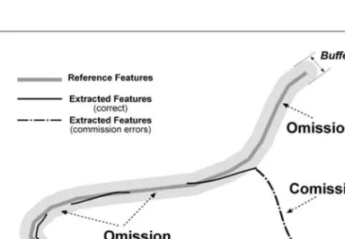
The proposed solution to the spatial registration problem and point-matching problem is to use a line lengthcomparison in-side a buffered reference theme. This approach addresses many of the characteristics of linear accuracy listed earlier. Although not a perfect solution for a final accuracy assess-ment, it is a tractable solution to the problem of model para-meterization. In the line-length buffer approach, a buffered distance commensurate with the spatial registration accuracy is specified (Figure 1). The total length of the extracted fea-tures located inside the buffered reference theme is compared to the total length of the reference lines inside the same buffer. One index of accuracy is the traditional “overall accuracy” value (also referred to as producer’s accuracy) computed as:
Overall Accuracy (%) * 100 (1)
where,
RoadsFEMTotal road length found by Feature Extraction Model (FEM).
RoadsRefTotal road length in Reference Data Set. With line length as the measure of correctness, however, it is possible for the overall accuracy to be greater than 100 percent. Even if the extracted feature set of roads are indeed essentially the same as the reference features, the extracted features may
RoadsFEM
Roads
Ref
Figure 1. The buffer-based calibration method for estimat-ing the percentage of agreement between a reference lin-ear transpor tation feature and candidate road segments extracted from an automated feature extraction program.
have a length slightly greater or shorter than the length in the reference set because of scale differences. More importantly, the percentage may be over 100 percent if the extracted fea-tures include commission error.
The overall accuracy in Equation 1 is a measure of only omissionerror. A comparison of extracted features and refer-ence features should also consider the commissionerror. In this study a measure of agreement is used that considers omis-sion and commisomis-sion errors. The formula used for considering both types of error simultaneously is defined as:
Road Feature Agreement (%)
* 100 (2) where,
RoadsFEMTotal road length found by Feature Extraction Model (FEM)
RoadsRefTotal road length in Reference Data Set RoadsFEM^ RoadsRefTotal FEM road length in Buffered
Area of Reference Data Set. This index for feature agreement is bounded between 0.0 and 1.0. Interpretation is as follows:
•
A value of 0.0 means no features in the reference data set are represented in the set extracted by the FEM.•
A value of 1.0 means the FEMset is identical to the population in the reference data set and neither set contains additional transportation features not in the other set.The index may also be interpreted as the percentage of the total features in both sets that is expressed in the common fea-ture set.
The method of using a buffered reference line as the “true line location” was proposed by Goodchild and Hunter (1997) for evaluating the spatial accuracyof a linear feature. Their goal was to determine the spatial accuracy measured in circu-lar statistics (e.g., circucircu-lar error probable) for the linear features in a theme. The buffer distance in their method was varied in an iterative fashion to converge on the probability threshold of interest (e.g., 68 percent, 90 percent) for the agreement in line length. Our use of the buffered theme is an inversion of the as-sumptions and known variables of the features in the Good-child and Hunter study. In GoodGood-child and Hunter’s work, the pairs of features (one in the extracted and one in the reference set) are known. The spatial accuracy is unknown. Our use of the buffered concept assumes the spatial accuracy is known while the pairs of features is unknown, i.e., an inversion of their assumptions. In the proposed accuracy assessment solu-tion, the buffered approach is applied to the entire setof refer-ence features simultaneously rather than individual features. As noted earlier, determining the specific paired FEMroad seg-ment and reference road segseg-ment is problematic. Also, the ap-plication of the buffered approach to individual roads would result in double counting of extracted road lengths in the over-lap buffer around road segment endpoints.
There are potential problems with using this buffered ref-erence theme approach for an accuracy assessment. As the buffer distance becomes large, the omission errors may be bi-ased by commission errors. Incorrectly identified transporta-tion features will occur inside large buffers, and their length will counteract the omitted transportation features; possibly resulting in an inflated accuracy. By using small buffer dis-tances, this problem is minimized, although not eliminated.
ORNLFeature Extraction Model
As a demonstration, the proposed parameterization model using the line-length buffered theme approach was coupled
RoadsFEM^ RoadsRef
Roads
FEMRoadsRef(RoadsFEM^ RoadsRef)
with the ORNLroad feature extraction model (FEM). The ORNL FEMis not the focus of this work as any road feature extraction model could be used. A brief presentation of the logic and pa-rameters of the ORNL FEMfollow.
The ORNL FEMfor extracting transportation features from panchromatic imagery is not a supervised approach; it is, in fact, an autonomous approach in the purest sense (Cheng, et al., 1998). It was developed to support work by the U.S. Air Force in a collaborative effort with ORNLand Northrop Grum-man Corporation. Imagery may be input to the system without any collateral information, such as spatial resolution, and without training sites. The model is designed to receive image input and extract transportation features.
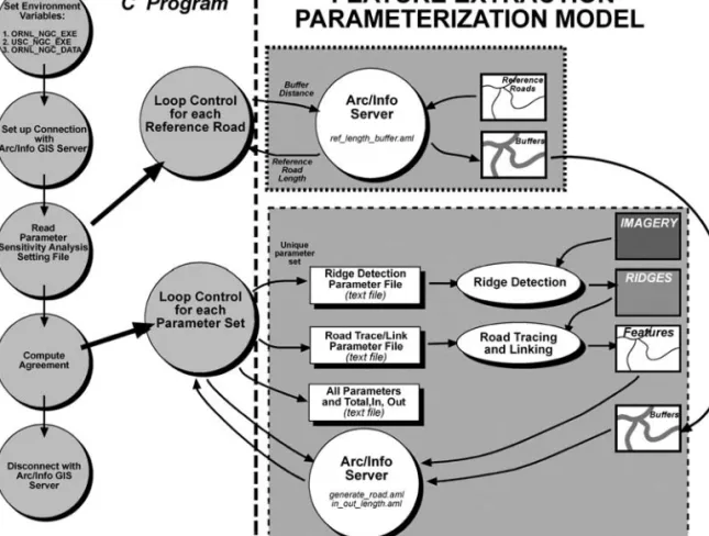
The ORNL FEMidentifies road segments in several stages (Figure 2). It contains several novel algorithms: ridge detec-tion, ridge thinning, and road linking and cleaning. Instead of following the conventional road detection approach, which uses edge detection and parallel edge finding (edges of road), a ridge (or valley) detector is used to extract roads. Roads typi-cally have a distinct appearance: a brighter (ridge) or darker (valley) strip with relative smooth and parallel borders. There are several advantages of detecting ridges over edges. First, a long, smooth strip in an image is very likely to be a manmade structure: a piece of road segment, canal, or runway. There-fore, the road extraction logic used after the ridge detection
Figure 2. Conceptual organization of processing steps in the transpor tation feature extraction model developed by the Oak Ridge National Laborator y.
will be simpler. Second, roads generally have a relatively con-sistent appearance regardless of the lighting and viewing di-rections. Therefore, the algorithm will be more stable. Twelve 5 5 templates representing 12 road directions were used to detect ridges and their associated orientations. The ridge like-lihood index and its direction at a pixel are taken when the convolution of the twelve templates reaches a maximum. Two matrices, ridge likelihood and ridge direction, are obtained in this process. In order to detect road with different widths, a pyramid scheme is used (Couloigner and Ranchin, 2000; Baumgartner, et. al., 1999). A low pass 3 3 mean filter is used to create coarser level images. At each level, all single width, linear features are detected and then transferred to the finer level.
The ridge segments obtained after applying ridge detec-tion are often represented by more than one pixel in width. The thinning (skeletonization) process obtains a simplified representation of the segments, probably including the posi-tions of the features they represent in the original image. Un-like the conventional image thinning operation performed on ridge likelihood images, a new image thinning algorithm works on the ridge direction image. In order to do so, a ridge connectivity index, which represents how well a pixel is con-nected with its neighboring pixel along the ridge direction, is determined at each pixel. The connectivity index at a pixel is a function of its orientation and its neighbors’ orientations. If a pixel’s orientation agrees with its neighboring pixels, it will have a higher connectivity value. On a ridge cross profile, the pixel with the highest connectivity value will be selected as a skeleton point. The advantages of this image thinning algo-rithm are:
•
It can better preserve a smooth image skeleton with fewer gaps,•
It does not require a threshold to cut off the weak and false pixels, and•
It is faster than most image thinning algorithms, which are iterative algorithms.The ridge image is traced and linked by chain codes. The extracted ridges are tested and cleaned by three criteria: curva-ture, isolation, and length. Chains in a raster data model are then converted to road segments in a vector data model. The final road features are created by applying another tracing and linking algorithm to the vector segments. The tracing and link-ing process is applied in a conservative way based on spatial proximity, orientation, and local geometry of the segments. For a given segment, all the segments encountered in the scanning area, which is a buffer along the segment, are collected as po-tential candidates. Similarity in image intensity value, similar-ity in ridge index value, similarsimilar-ity in orientations at the ex-tremities of the gap, and the length of the gap are used to elevate the candidacy of the segments. Short and isolated seg-ments are removed because they are very unlikely a part of a road network.
The ORNL FEMalso included an autonomous image rectifi-cationstep. The extracted road features are used to automati-cally rectify the image to reference roads. The only assump-tion is the original image is “in the general study area,” and some common road reference features exist. After the rectifi-cation process is performed, the rectified road features are then used to populate a transportation feature database.
Since an assumption in the parameterization model is that the spatial accuracy of the image is known a priori, the model can only be used if the imagery is rectified. In the case of the ORNL FEM, the model would first be parameterized, and then the parameterized model run on un-rectified imagery. In our use of the ORNL FEM, we omitted the autonomous rectifica-tion step; rectified imagery rather than un-rectified imagery was used as input.
Implementation of Parameterization Model
The parameterization model presented above was imple-mented using a combination ofUNIXshell scripts, C programs, and Arc Macro Language©(AML) programs. The
implementa-tion is a tightly-coupled approach between aGISandORNL FEM. The structure of this approach is graphically displayed in Figure 3.
The model was implemented as a client/server system, where the parameterization model is a client andARC/INFO©is a server. The communication between the model andARC/ INFO©server was based on a client/server C-library provided byARC/INFO©. The library itself is based on Remote Procedure Call (RPC), which is one of many mechanisms ofUNIXprocess communication. Generating parameter configurations, execut-ing the ridge detection and road segment tracexecut-ing programs, converting from image coordinates to map coordinates, and calculating accuracy indexes are the main tasks in the client part. TheARC/INFO©server is responsible for generating buffers around the reference roads and, initially, overlaying the ex-tracted roads with the buffered reference roads to calculate the length inside and outside the buffer. For efficiency reasons, the overlay and length calculation were re-implemented as a C-program which is about 30 times faster than theARC/INFO© server.
The results of the sensitivity model and all parameter val-ues are stored in a separate ASCIIfile (Table 1). In the current implementation thirteen of the fields are the parameter values used in ridge detection and road segment tracing. The next three fields are total length of the reference road, the road length inside and length outside reference buffers. The last two fields are the overall accuracy and the feature agreement indexes. Each record represents a unique parameter configura-tion. The output file contains the results of every parameter combination. The “best” parameter value set is easily found through a table sort operation. Because the search for the best set is an exhaustive search, alternative near-best solutions are easily identified.
The parameterization model shown in Figure 3 creates an ASCIIfile containing the parameter configuration and accuracy results for each unique parameter set. On a full-scale test, this data set may contain over 12,000 records. After examining the model results, it is often desirable to then select a specific model configuration and view the results of one of the model runs (Figure 4). While the sensitivity model analyzes all para-meter combinations, it does not save the extracted roads from each model run (the data storage requirements would be ex-ceedingly large). An ArcView©project with accompanying
Av-enue©and C-code were implemented to allow the user to
se-lect a specific parameterization and automatically execute the model to produce the extracted roads from this parameteriza-tion.
Example Calibration
Image data and reference data of various types were assembled for performance testing of theORNL FEM. Digital orthophotogra-phy (1 m1 m) of the Oak Ridge Reservation (ORR) was used as an example. Coarser resolutions (from 1 m to 10 m by 1 m steps) of the imagery were artificially created through spatial averaging. Class one through five transportation features were defined as in theUSGSDigital Line Graph (DLG) classification scheme. Reference data were compiled through visual inter-pretation of the photography for theORR. The buffer radius commensurate with the approximate spatial accuracy of the 3 m3 m imagery used as an example in this article was 10 m. Based on available information on the expected performance of theFEM, we conducted numerous calibration tests with se-lected values for the seven key parameters of theFEM. These seven parameters, their ranges, and examined values are
Figure 3. Conceptual organization of the data processing involved in the coupled FEMand parameteriza-tion model.
TABLE1. PARAMETERSEXAMINED IN THESEVEN-PARAMETERFEM SENSITIVITYANALYSIS
Initial Values Examined in Category Name Range Default Sensitivity Analysis Image enhancement hist_power 0.8–2.5 1.0 0.5, 1.0, 1.5
hist_tilesize 9–2048 2048 hist_remap_size 1–2048 2048
Line filter sensi_index 0–16 8 2, 4, 6, 8, 10, 12, 14, 16 max_levels 1–3 3
min_bv 80–120 100
min_count 0–10 5 1, 3, 5
std_ratio 1–25 10 1, 5, 10, 15, 20, 25 max_link_index 0–12 6
Chain code tracing min_ridge_index 2–30 20
max_curv 2–3.0 2.5 2.5, 3.0, 3.5 min_curv 0–0.5 0.1 0, 0.02 min_length 20–40 (pixel) 40 5, 10, 20, 30 Vector gap filling split_dist 2–10 (pixel) 2
split_angle 150–180 170 fan_angle 0–90 60 fan_radius 0–50 (pixel) 40 seg_angle 120–180 150 mean_diff 0–50 30
shown in Table 1. The number of unique parameterized mod-els for each image was 10,368.
An example of the extraction accuracy by variation in val-ues of these seven parameters for a 3 m image within the ORR is illustrated in Figure 4. Maximum feature agreement for the
3 m imagery was 87 percent. When the goal is maximizing feature agreement (high accuracy with low commission er-rors), the ideal histogram power ranged from 0.5 to 1.0. The ideal sensitivity index ranged from 14 to 16 for this same image resolution. For this 3 m image, slight changes in the
other parameter values have little effect on extraction agree-ment.
Artificial degradation of the ORR3 m 3 m image to coarser resolutions (5 m to 10 m) produced new findings. Small changes in the optimized parameter values for the 5 m imagery were found to result in large changes in extraction agreement with 10 m imagery. The maximum extraction agre-ement for the 5 m imagery would use a sensitivity index be-tween 10 and 12. The best values for the histogram power vary dramatically with image resolution, from 0.8 to 2.3. For the 10 m imagery, the range in histogram power and sensitiv-ity index values is much greater although the incremental val-ues within this range result in dramatic differences in extrac-tion agreement.
Summary
The proposed buffered reference theme approach solves sev-eral problems in model calibration, sensitivity analysis, and accuracy assessment phases. First, it allows for a digital extrac-tion accuracy assessment without visual analysis. This digital accuracy assessment then provides for an autonomous accu-racy assessment. Third, because the assessment is completely autonomous, this approach addresses the basic problem of a large number of parameter combinations. The approach uses a vector data model and incorporates the known spatial error in the reference data. Finally, once a collection of images and ref-erence themes has been established, evolutionary changes in the feature extraction model may be easily evaluated.
The parameterization model does have limitations, how-ever. Commission errors can occur within the buffered area. This may be observed when nearby non-transportation fea-tures, such as powerlines, are inadvertently identified as dirt roads. The model does not include other characteristics of
agreement, such as segments or gaps in road segments. Fu-ture studies using imagery of a variety of geographic envi-ronments and imagery types could be performed to assess the stability of the buffered reference theme approach for model calibration.
Acknowledgments
We would like to express our appreciation for the assistance in this work from John Smyre and Richard Durfee of the Oak Ridge National Laboratory.
References
Agouris, P., A. Stefanidis, and S. Gyftakis, 2001. Differential snakes for change detection in road segments, Photogrammetric Engi-neering & Remote Sensing, 67(12):1391–1399.
Baumgartner, A., C. Steger, H. Mayer, W. Eckstein, and H. Ebner, 1999. Automatic road extraction based on multi-scale, grouping, and context, Photogrammetric Engineering & Remote Sensing, 65(7): 777–785.
Cheng, Y., J. Smyre, M. Hodgson, and X. Li, 1998. Feature extraction, image registration, and transportation data base population and update, Oak Ridge National Laboratory Technical Report. Couloigner, I., and T. Ranchin, 2000. Mapping of urban areas: A
mul-tiresolution modeling approach for semi-automatic extraction of streets, Photogrammetric Engineering & Remote Sensing, 66(7): 867–874.
Goodchild, M.F., and G.J. Hunter, 1997. A simple positional accuracy measure for linear features, International Journal of Geographical Information Systems, 11(3):299–306.
Wang, J., P.M. Treitz, and P.J. Howarth, 1992. Road network detection from SPOT imagery for updating geographical information sys-tems in the rural-urban fringe,International Journal of Geograph-ical Information Systems, 6(2):141–157.
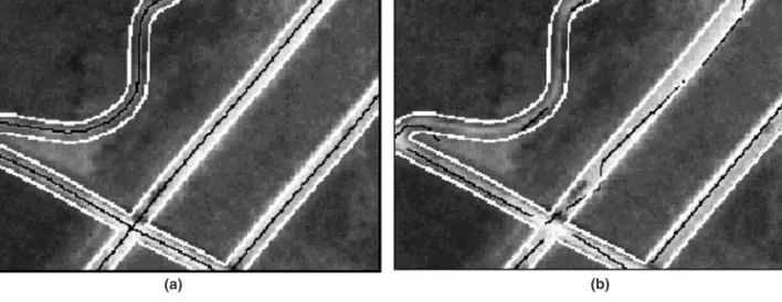
Figure 4. Example of raw image (a), and extracted road feature segments (b) for a por tion of a 3 m 3 m digital or thoimager y on the Oak Ridge Reser vation. This par ticular examples illustrates the problem of line gaps and spatial differences between extracted versus reference road segments.