A New Data Clustering Approach for Data Mining in Large Databases
Cheng-Fa Tsai
†, Han-Chang Wu, and Chun-Wei Tsai
Department of Management Information Systems,
National Pingtung University of Science and Technology, Pingtung, Taiwan, 91201
Email:
[email protected]
Abstract
Clustering is the unsupervised classification of patterns (data items, feature vectors, or observations) into groups (clusters). Clustering in data mining is very useful to discover distribution patterns in the underlying data. Clustering algorithms usually employ a distance metric based similarity measure in order to partition the database such that data points in the same partition are more similar than points in different partitions. In this paper, we present a new data clustering method for data mining in large databases. Our simulation results show that the proposed novel clustering method performs better than the Fast SOM combines K-means approach (FSOM+K-means) and Genetic K-Means Algorithm (GKA). In addition, in all the cases we studied, our method produces much smaller errors than both the FSOM+K-means approach and GKA.
Index Terms: Clustering、data mining、SOM、k-means、ant system
1. Introduction
The problem of clustering has become increasingly important in recent years. The clustering problem has been addressed in many contexts and by researchers in many disciplines; this reflects its broad appeal and usefulness as one of the steps in exploratory data analysis. Clustering approaches aim at partitioning a set of data points in classes such that points that belong to the same class are more alike than points that belong to different classes. These classes are called clusters and their number may be preassigned or can be a parameter to be determined by the algorithm. There exist applications of clustering in such diverse fields as business, pattern recognition, communications, biology, astrophysics and many others. Cluster analysis is the organization of a collection of patterns (usually represented as a vector of measurements, or a point in a multidimensional space) into clusters based on similarity. Usually, distance measures are utilized. Data clustering has its roots in a number of areas, including data mining, machine learning, biology, and statistics.
Traditional clustering algorithms can be classified into two main categories: hierarchical and partitional [1]. In hierarchical clustering, the number of clusters need not be specified a priori, and problems due to initialization and local minima do not arise. However, since hierarchical methods consider only local neighbors in each step, they cannot incorporate a priori knowledge regarding the global shape or size of clusters. As a result, they cannot always separate overlapping clusters. In addition, hierarchical clustering is static, and points committed to a given cluster in the early stages cannot move to a different cluster.
Prototype-based partitional clustering algorithms can be divided into two classes: crisp clustering where each data point belongs to only one cluster, and fuzzy clustering where every data point belongs to every cluster to a certain degree [2]-[3]. Fuzzy clustering algorithms can deal with overlapping cluster boundaries [19]-[21]. Partitional algorithms are dynamic, and points can move from one cluster to another. They can incorporate knowledge regarding the shape or size of clusters by using appropriate prototypes and distance measures. Most partitional approaches utilize the alternating optimization techniques, whose iterative nature makes them sensitive to initialization and susceptible to local minima. Two other major drawbacks of the partitional approach are the difficulty in determining the number of clusters, and the sensitivity to noise and outliers [4].
Clustering can be generally defined as the following problem. Given N points in d dimensional feature space, find interesting groups of points. Many algorithms assume that
the number of clusters, k, is known a priori and find the k
clusters that minimize some error metric.
Inspired by the collective behavior of a real ant colony, Dorigo first presented the Ant System (AS) in his paper [30], and the study was further continued by him [27]-[29], [31]. The characteristics of an artificial ant colony include positive feedback, distributed computation, and the use of a constructive greedy heuristic. Positive feedback accounts for rapid discovery of good solutions, distributed computation avoids premature convergence, and the greedy heuristic helps find acceptable solutions in the early stages of the search process. In order to demonstrate the AS method, the authors
apply this method to the classical traveling salesman problem (TSP), quadratic assignment problem (QAP), and job-shop scheduling problem. AS reveals very good results in each applied area. More recently Dorigo and Gambardella have been working on extended versions of the AS paradigm. Ant system is one of the extensions and has been applied to the symmetric and asymmetric TSP with excellent results [27]. The AS has also been applied with success to other combinatorial optimization problems such as the scheduling, partitioning, coloring, telecommunications networks, and vehicle routing problem [5]-[8].
2. Definitions for Clustering Problem
A clustering C means partitioning a data set into a set of
clusters Ci, i = 1,…, H. A widely adopted definition of
optimal clustering is a partitioning that minimizes distances within and maximizes distances between clusters. Within- and between-clusters distances can be defined in several ways; see [37]. In this paper, Euclidean norm is utilized because it is widely utilized with SOM (Self-Organizing Feature Map). In addition, the k-means error criterion is based on it. In order to evaluate the proposed method, we define the time cost for clustering as follows, n r i i i r Te Ts Ta n
∑
= − = 1 ) ( ,where Ta represents the time cost for clustering,
r
n denotes the number of runs, Ts is the initial time for clustering, Terepresents the terminate time for clustering.
3. Ant Colony Optimization (ACO)
The ant colony optimization technique has emerged recently as a novel meta-heuristic belongs to the class of problem-solving strategies derived from natural (other categories include neural networks, simulated annealing, and evolutionary algorithms) [9]-[18], [22], [25], [32]-[36]. The ant system optimization algorithms is basically a multi-agent system where low level interactions between single agents (i.e., artificial ants) result in a complex behavior of the whole ant colony. Ant system optimization algorithms have been inspired by colonies of real ants, which deposit a chemical substance (called pheromone) on the ground. It was found that the medium used to communicate information among individuals regarding paths, and used to decide where to go, consists of pheromone trails. A moving ant lays some pheromone (in varying quantities) on the ground, thus making the path by a trail of this substance. While an isolated ant moves essentially at random, an ant encountering a previously laid trail can detect it and decide with high probability to
follow it, thus reinforcing the trail with its own pheromone.
The collective behavior where that emerges is a form of autocatalytic behavior where the more the ants following a trail, the more attractive that trail becomes for being followed.
The process is thus characterized by a positive feedback loop, where the probability with which an ant choose a path increases with the number of ants that previously chose the same path.
Given a set of n cities and a set of distances between them, the Traveling Salesman Problem (TSP) is the problem of finding a minimum length closed path (a tour), which visits
every city exactly once. We call dij the length of the path
between cities i and j. An instance of the TSP is given by a graph (N, E), where N is the set of cities and E is the set of edges between cities (a fully connected graph in the Euclidean TSP).
Let bi(t) (i = 1,…,n) be the number of ants in city i at
time t and let ∑
=
= n i bit m
1 () be the total number of ants. Let
)
(t n
ij +
τ be the intensity of pheromone trail on connection (i, j)
at time t + n, given by
τij(t+n)=(1−ρ)τij +∆τij(t,t+n), (1)
where
ρ
is a coefficient such that 1-ρ
denotes a coefficientwhich represents the evaporation of trail between time t and t +
n,
∑
=∆ + = + ∆ m k k ij ij(t,t n) 1 τ (t,t n) τ , where k t t n ij + ∆τ (, ) is thequantity per unit of length of trail substance (pheromone in real ants) laid on connection (i, j) by the kth ant at time t + n and is
given by the following formula: ∈ = ∆ otherwise 0 by tabu described tour ) , if(i j k L Q k k ij τ (2)
where Q denotes a constant and Lk represents the tour length found by the kth ant. For each edge, the intensity of trail at time 0 (τij(0)) is set to a very small value.
While building a tour, the transition probability that ant k
in city i visits city j is
[ ] [ ]
[
] [ ]
⋅ ⋅ =∑
∈ 0 ) ( ) ( ) ( α β β α η τ η τ ik ik allowed k ij ij k ij t t t p k otherwise ) ( allowed if j ∈ k t (3)where allowedk(t) is the set of cities not visited by ant k at time t, and ηijdenotes a local heuristic which equal to 1/d (and it is
called ‘visibility’). The parameterαand β control the
relative importance of pheromone trail versus visibility. Hence, the transition probability is a trade-off between visibility, which says that closer cities should be chosen with a higher probability, and trail intensity, which says that if the
connection (i, j) enjoys a lot of traffic then is it highly
profitable to follow it.
A data structure, called a tabu list, is associated to each ant in order to avoid that ants visit a city more than once. This list tabuk(t) maintains a set of visited cities up to time t by
follows: allowed (t) {j|j tabu (t)}
k
k = ∉ . When a tour is
completed, the tabuk(t) list (k = 1,…, m) is emptied and every
ant is free again to choose an alternative tour for the next cycle. By using the above definitions, we can describe the ant colony optimization algorithm as follows:
procedure ACO algorithm for TSP
Set parameters, initialize pheromone trails
while (termination condition not met) do
Construct Solutions Apply Local Search Local_Pheromone_Update End
Global_Pheromone_Update
end ACO algorithm for TSPs
Fig. 1. The ACO algorithm.
4. The
proposed
Approach
In this paper, we propose a novel ant system with differently favorable strategy for data clustering. To the best of our knowledge, there is no existing ant colony optimization algorithm for data clustering. It is desirable to design an ant colony optimization algorithm (ACO) that is not required to solve any hard subproblem but can give nearly optimal solutions for data clustering. The proposed method can obtain optimal solutions quicker via differently favorable strategy. The ant colony optimization with different favor (ACODF) algorithm has the following three important desirable strategies: (a) using differently favorable ants to solve the clustering problem, (b) adopting simulated annealing concept for ants to decreasingly visit the amount of cities to get local optimal solutions, (c) utilizing tournament selection strategy to choose a path. According to our simulation results, the computation cost and error rate of our proposed method can reduce much more than the other promising methods:
FSOM+K-means (fast self-organizing map combines k-means)
[15] and GKA (genetic K-means algorithm) [23].
4.1. The Strategy of Using ACO with Different favor
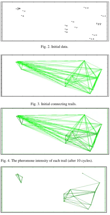
We utilize ACO with different favor to solve the clustering problem. Every ant only needs to visit (1/10) cities not all of cities; then, the ant decreasingly visit cities every time. After several iterations (cycles), the trail intensity (pheromone) close between nodes of trails will be increased; on the other hand, the trail intensity (pheromone) far between nodes of trails will be decreased. Therefore, ants will favor to visit the closer nodes and then reinforcing the trail with their own pheromone. Finally, a number of clans (clusters) will be built. Fig. 2 through Fig. 5 illustrates the clustering processes using the strategy of ACO with different favor. Fig. 2 shows the initial data; Fig. 3 reveals the initial connecting trails; Fig. 4 depicts the pheromone intensity of every trail after 10 cycles; while the trails with higher pheromone intensity after 10 cycles are shown in Fig. 5.
Fig. 2. Initial data.
Fig. 3. Initial connecting trails.
Fig. 4. The pheromone intensity of each trail (after 10 cycles).
Fig. 5. The trails with higher pheromone Intensity (after 10 cycles).
4.2. The Strategy of Using Simulated Annealing
We adopt simulated annealing concept for ants to decreasingly visit the number of cities to get local optimal solutions. Thus, two useful formulas are devised as follows, ns(t+1)=ns(t)×T, (4)
where ns is the number of visiting nodes of ants during T0
function (see the detailed algorithm in Fig. 7), ns(t+1) denotes the current number of visiting nodes of ants, ns(t) represents the number of visiting nodes of ants at last time (cycle), T is a constant (T= 0.95). According to this formula, we understand the fact that ants really decreasingly to visit cities. Eqn. (5) shows the relationship between nf(t+1) and ns(t), where nf is
t h e n u mb e r o f v i s i t i n g n o d e s o f a n t s d u r i n g T1
function (see the detailed algorithm in Fig. 7), nf(t+1) denotes the current number of visiting nodes of ant, nf(t) represents the number of visiting nodes of ant at last time (cycle), run = 2,
i∈{1, 2}. 3 ) ( 3 ) ( 2 ) 1 ( ⋅ ⋅ − ⋅ = + run t ns i t ns t nf , (5)
4.3. The Strategy of Using Tournament Selection
A scheme called Roulette Wheel Selection is one of the most common techniques being used for a proportionate selection mechanism. Traditional ACO also uses this technique to select trials. However, Tournament Selection is more powerful than Roulette Wheel Selection in our experiences. Therefore, we adopt it in our research. Fig. 6 reveals this mechanism. In Fig. 6, suppose we randomly select three lines among five lines; then, we continue to select the shortest line among the three previous selected lines (in this
instance means SE). A B C D E S Selected Line Unselect Line A B C D S SA SD SE random select E B C D E S best A SE a) b) c)
Fig. 6. The tournament selection mechanism.
4.4. The Proposed Algorithm for Clustering The proposed algorithm for clustering is shown as follows,
void main() {
Initialization(); //initial the data set Do
{
T0(); //let each ant to visit some data set cities at random
For i=1 to run //run = 2
T1i(); // follow the pheromone of T11() and T12() to visit cities
For every edge (i, j) update the
∆
τ
ijgiven by Eq.(2) } While (ACODF.stop=Ture)Consolidation();
Compute the clustering results to find clusters ; }
Void Initialization() {
For i=1 to n Input data set;
For every edge(i, j) set
∆
τ
ij=0Place m ants randomly to m nodes; // m is equal to (1/2) n
} void T0 () {
For k=1 to m {
For l=1 to ns(t) randomly choose city j to move, where ns(t) is given by Eqn. (4) // decreasing rate is 0.95 and the initial number of visiting nodes is equal to
(1/15) n
Compute Lk for the kth ant
Put
∆
τ
ij to the edge from kth ant visited}Set visiting range of T1 //to set upper bound and lower bound } void T1i() { Set nf(t+1) = ) 3 ) ( ( ) ( ) 3 / 2 ( ⋅ ⋅ − ⋅ run t ns i t ns For k=1 to m {
Choose city j to tournament selection
// randomly selected 10 (j=10) trails and find the high quality pheromone trail, select this trail to visit
Compute Lkfor the kth ant Put
∆
τ
ij to edge from kth ant visited}}
void Consolidation() {
Compute pheromone quality of every trail and set the trail state //to set visible (greater than the average of all trails pheromone
quality) and non-visible trails (less than the average of all trails pheromone quality) and set empty the pheromone quality trail is not exist
Using visible trails to find all clusters Compute nearest distances for clusters Join the small cluster with the nearest cluster }
Fig. 7. The proposed ACODF algorithm.
5. Simulation
Results
In order to verify the performance of our method, some computer simulations have been conducted on a PC Pentium
Ⅲ. We are even more to conduct a non-spherical clustering
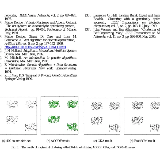
with 579 data set and a spherical clustering with 400 data set. Fig. 8 depicts 400 source data set and the results of a spherical
clustering with 400 data set utilizing the FSOM+K-means,
ACODF, and GKA approaches, respectively. Table 1 shows the simulation results regarding between-clusters distances (define by [37]) of a non-spherical clustering with 579 data set
for FSOM+K-means, ACODF, and GKA. Table 2 reveals the
comparison of time cost for FSOM+K-means, ACODF, and
GKA. It is observed that ACODF searches faster than some of the other promising evolutionary algorithms used for clustering. The time cost in non-spherical clustering with 579 data set for ACODF and GKA almost the same. However,
ACODF can always search faster than FSOM+K-means and
GKA in sphere clustering with 300 and 400 data set. In addition, according to the results of clustering comparisons from Fig. 8 and Table 1 to Table 4, it is observed in the simulations that ACODF converges to the best known optimum
or near-optimum (with no error rate or lower error rate) corresponding to the given data in concurrence with the convergence result.
6. Conclusions
In this paper, we propose a novel algorithm called ant colony optimization with different favor (ACODF) for data clustering. The ACODF algorithm has the following three important desirable strategies: (a) using ACO with different favor to solve the clustering problem, (b) adopting simulated annealing concept for ants to decreasingly visit the amount of cities to get local optimal solutions, (c) utilizing tournament selection strategy to choose a path. We compare our ACODF
method with the FSOM+K-means approach and GKA.
Through experiments, we show that ACODF efficiently finds accurate clusters in large high dimensional datasets.
7. References
[1]. A.K. Jain and R.C. Dubes, Algorithms for clustering
data, Englewood Cliffs, N.J.: Prentice Hall, 1988.
[2]. Hichem Frigui and Raghu Krishnapuram, "A robust
competitive clustering algorithm with applications in
computer vision," IEEE Transactions of Pattern
Analysis and Machine Intelligence, vol. 21, no. 5, pp. 450-465, May 1999.
[3]. J.-H. Wang and J.-D. Rau,"VQ-Agglomeration: a novel
approach to clustering," IEE Proc.-Vis., Image Signal Process., vol. 148, no. 1, pp. 36-44, February 2001. [4]. Sudipto Guha , Rajeev Rastogi and Kyuseok
Shim,"CURE: An efficient clustering algorithm for large database," Information Systems (Elsevier Science), vol. 26, no. 1, pp. 35-58, 2001.
[5]. Randall S. Sexton and Robert E. Dorsey, "Reliable
classification using neural networks: a genetic algorithm
and backpropagation comparision,” Decision Support
System, vol. 30, pp. 11-22, 2000.
[6]. Kimmo Uutela, Matti Hämäläinen and Riitta Salmelin,"Global Optimization in the Localization of
Neuromagnetic Sources," IEEE Transactions on
Biomedical Engineering, vol. 45, no. 6, pp. 716-723, 1998.
[7]. Hiroshi Ishikawa , Manabu Ohta and Koki
Kato,"Document Warehousing: A document-intensive
application of a multimedia database," Eleventh
International Conference on Data Engineering, pp. 25 -31, 2001.
[8]. L. Lucchese and S.K. Mitra, 1999 IEEE International
Conference on Content-Based Access of Image and Video Libraries, pp. 74 -78, 1999.
[9]. T. Kohonen, "Self-organized formation of topologically correct feature maps,"Biol. Cybern., vol. 43, pp. 59-69, 1982.
[10]. T. Kohonen, "The self-organizing map", Proc. IEEE, vol. 78, no. 9, pp. 1461-1480, 1990.
[11]. K.Obu-Cann, K. Iwamoto, H. Tokutaka and K. Fujimura,
"Clustering by SOM (self-organising maps), MST (minimal spanning tree) and MCP (modified
counter-propagation)," 6th IEEE International
Conference on Neural Information Processing, pp. 986-991, vol. 3, 1999.
[12]. Philipp Tomsich,, Andreas Rauber and Dieter Merkl,
"Optimizing the parSOM neural network implementation for data mining with distributed
memory systems and cluster computing," IEEE 11th
International Database and Expert Systems Applications , pp. 661-665, 2000.
[13]. Masahiro Endo, Masahiro Ueno, Takaya Tanabe and
Manabu Yamamoto, M., "Clustering method using
self-organizing map", IEEE Neural networks for Signal Processing, vol. 1, pp. 261-270, 2000.
[14]. Hiroshi D0uzono, Shigeomi Hara and Yoshio
Noguchi,"A clustering method of chromosome
fluorescence profiles using modified self organizing
map controlled by simulated annealing," IEEE
International Joint Conference on Neural Networks, vol. 4, pp.103-106, 2000.
[15]. Mu-Chun Su and Hsiao-Te Chang, "Fast self-organizing feature map algorithm", IEEE Transactions on Neural Networks, vol. 11, no. 3, pp. 721-733, May 2000.
[16]. Mu-Chun Su and Hsiao-Te Chang, Machine Learning:
Neural Network, Fuzzy System and Genetic Algorithms, Taiwan:OpenTech, 1999.
[17]. S.P. Lloyd, “Least squares quantization in pcm",
Transaction on Inform. Theory, vol. 28, no. 2, pp. 129-137, 1982.
[18]. Chinrungrueng C. and Qequin C.H.,"Optimal adaptive
k-means algorithm with dynamic adjustment of learning rate," IEEE Transaction on Neural Networks, vol. 6, no. 1, pp. 157-169, Jan 1995.
[19]. J.Bezdek and R. Hathaway, "Numerical convergence
and interpretation of the fuzzy C-Shells clustering algorithm,"IEEE Transactions on Neural Networks, vol. 3, pp. 787-793, Sept. 1992.
[20]. R.Krishnapuram, O. Narsraoui and H. Frigui, "The
fuzzy C spherical shells algorithm: A new approach,"
IEEE Trans. Neural Networks, vol. 3, pp. 787-793, Setp. 1992.
[21]. Il Hong Suh, Jae-Hyun Kim and Frank Chung-Hoon Rhee, "Convex-Set-Based Fuzzy Clustering," IEEE Transactions on Fuzzy System, vol. 7, no. 3, pp. 271-285, JUNE 1999.
[22]. Rajeev Kumar and Peter Rockett, "Multiobjective
genetic algorithm partitioning for hierarchical learning of high-dimensional pattern spaces: a
learning-follows-decomposition strategy," IEEE
Transactions on Neural Networks, vol. 9, no. 5, pp. 822-830, September 1998.
[23]. K.Krishna and M. Narasimha Murty, "Genetic K-means
algorithm, " IEEE Transactions on System, Man and
Cybernetics-Part B: Cybernetics, vol. 29, no. 3, pp. 433-439, 1998.
[24]. R.C. Dubes and A.k. Jain. Algorithms for Clustering
Data, Prentice Hall, 1988.
[25]. K. Alsabti, S. Ranka, and V. Singh, "An efficient
K-means clustering algorithm,” PPS/SPDP Workshop on High performance Data Mining, 1997.
[26]. Chedsada Chinrungrueng and Carlo H. Sequin,
"Optimal adaptive K-means algorithm with dynamic
adjustment of learning rate," IEEE Transaction on
Neural Networks, vol. 6, no. 1, January 1995.
[27]. Marco Dorigo , Vittorio Maniezzo and Alberto Colorni,
"Ant system: optimization by a colony of cooperating
agents," IEEE Transaction on System, Man and
Cybernetics-Part B, vol. 26., no. 1, pp. 29-41 February 1996.
networks," IEEE Neural Networks, vol. 2, pp. 887-891, 1997.
[29]. Marco Dorigo , Vittorio Maniezzo and Alberto Colorni,
"The ant system: an autocatalytic optimizing process," Technical Report, pp. 91-016, Politecnico di Milano, Italy, 1991
[30]. Marco Dorigo, Gianni Di Caro and Luca M. Gambardella, "Ant algorithm for discrete optimization," Artifical Life, vol. 5, no. 2, pp. 137-172, 1999.
[31]. http://iridia.ulb.ac.be/~mdorigo/ACO/ACO.html
[32]. J. H. Holland, Adaption in Natural and Artificial System, Boston, MA: MIT Press, 1992.
[33]. M. Mitchell, An introduction to genetic algorithms,
Cambridge, MA: MIT Press, 1996.
[34]. Z. Michalewicz, Genetic Algorithms + Data Structures
= Evolution Programs, New York: Springer-Verlag, 1994.
[35]. K. F. Man, K.S. Tang and S. Kwong, Genetic Algorithms,
Springer-Verlag 1999.
[36]. Lawrence O. Hall, Ibrahim Burak Özyurt and James C.
Bezdek, "Clustering with a genetically optimized
approach," IEEE Transactions on Evolutionary
computation, vol. 3, no. 2, pp. 103-112 July 1999. [37]. Juha Vesanto and Esa Alhoniemi, “Clustering of the
Self-Organizing Map,” IEEE Transactions on Neural
Networks, vol. 11, no. 3, pp. 586-600, May 2000.
(a) 400 source data set (b) ACODF result (c) GKA result (d) Fast SOM result
Fig. 8. The results of a spherical clustering with 400 data set utilizing ACODF, GKA, and FSOM+K-means.
Table 1: THE BETWEEN-CLUSTER RESULTS OF A NON-SPHERICAL CLUSTERING WITH 579 DATA SET USING ACODF, GKA, AND FSOM+K-MEANS.
Between-clusters single linkage complete linkage average linkage centroid linkage error rate
FSOM
+k-means
0.029666033 0.866149859 0.439210384 0.456982684 0.031826ACODF 0.030057599 0.866149859 0.43637177 0.455576274 0.001727
GKA 0.029666033 0.866149859 0.439210384 0.456982684 0.031826
Table 2: THE COMPARISON OF TIME COST FOR FSOM+K-MEANS, ACODF, AND GKA.
579(non-spherical) 300 (spherical) 400 (non spherical)
FSOM
+k-means
8097 sec. 8155 sec. 8234 sec.ACODF 2320 sec. 782 sec. 1531 sec.