Assessment of optical systems by means of point-spread
functions
Joseph J.M. Braat, Sven van Haver
Optics Research Group, Technical University Delft, Lorentzweg 1, 2628 CJ Delft, The Netherlands
Augustus J.E.M. Janssen, Peter Dirksen
Philips Research Europe, HTC 36 / 4, 5600 JA Eindhoven, The Netherlands
To be published in:
Progress in Optics, Vol. 51, Ed. E. Wolf, Elsevier, Amsterdam / The Nether-lands, 2008
Contents
1 Introduction 4
1.1 The optical point-spread function 5
1.2 Quality assessment by inverse problem solving 7 2 Theory of point-spread function formation 9
2.1 Field representations and the diffraction integral 9 2.2 The Debye integral for focused fields 13
2.3 The Rayleigh-I integral for focused fields 15 2.4 Comparison of the various diffraction integrals 17
2.5 The amplitude of the point-spread function produced by an optical system 21 2.6 Analytic expressions for the point-spread function in the focal region (scalar case) 29
2.7 Analytic expressions for the point-spread function in the vector diffraction case 37 2.8 The point-spread function in a stratified medium 42
3 Energy density and power flow in the focal region 45 3.1 Expression for the electric energy density 46
3.2 Expression for the Poynting vector 57 4 Quality assessment by inverse problem solution 64
4.1 Intensity measurements and phase retrieval 65 4.2 The optical inverse problem for finite-aperture imaging systems 66
4.3 Solving the optical inverse problem using phase diversity 70 5 Quality assessment using the Extended Nijboer-Zernike diffraction theory 73
5.1 Scalar retrieval process using the Extended Nijboer-Zernike theory 74 5.2 Pupil function retrieval for high-NA imaging systems 87
5.3 Retrieval examples for high-NA systems 90
6 Conclusion and outlook 109
A Derivation of Weyl’s plane wave expansion of a spherical wave 111 B The Debye integral in the presence of aberrations 112
C Series expansion of the diffraction integral at large defocus 114 D Series expansion for the diffraction integralVm
n,j(r, f) 115
D.1 Expansion using the functionsVm
n (r, f) 115
D.2 Expansion using the functionsTm
n (r, f) 116
E The predictor-corrector procedure 118 F Zernike coefficients for circularly symmetric polarization states 120
1 Introduction
The subject of this chapter is the computation of the point-spread function of optical imaging systems and the characterization of these systems by means of the measured three-dimensional structure of the point-spread function. The point-spread function, accessible in the optical domain only in terms of the energy density or the energy flow, is a nonlinear function of the basic electro-magnetic field components in the focal region. That is why the reconstruction of the amplitude and phase of the optical far-field distribution that produced a particular intensity point-spread function is a nonlinear procedure that does not necessarily have a unique solution.
For a long time, a detailed measurement of the point-spread function was not possible because of the lack of adequate intensity recording media. The eye of a human subject, although close to perfection over the typical diameter of its iris, is not capable of appreciating the small imperfections that may be present in high-quality instruments for optical observation. In the seventeenth and eighteenth century, telescopes and microscopes were still manufactured in a craftmanship way, without the feedback from reliable and objective op-tical measurement. Generally speaking, one could say that he modern epoch of high-quality instrument making has started with the pioneering work by Joseph von Fraunhofer who combined his gifts in optical design with a profes-sional approach to optical measurement technology and manufacturing. In a few decades, as of 1850, the trial-and-error methods from the past were ruled out and scientific instrument making was gradually introduced. Nowadays, the perfection of optical instruments has reached a level that was thought to be impossible in the still recent past, see the statement in [Conrady (1929)]: ”it is no use to acquire a microscope objective with a numerical aperture beyond 0.80 because a still larger cone of light will only contribute to light gathering and not to improved imaging”. Especially since the 1970’s, the quality of opti-cal imaging systems (telescopes, microscope objectives, high-quality projection lenses for optical lithography, space observation cameras) has been pushed to the extreme limits. At this level of perfection, a detailed analysis of the opti-cal point-spread function is necessary to understand the image formation by these instruments, especially when they operate at high numerical aperture. In terms of the imaging defects, we are allowed to suppose that the wavefront aberration of such instruments is not substantially larger than the wavelength
λ of the light. In most cases, the aberration even has to be reduced to a minute fraction of the wavelength of the light to satisfy the extreme specifications of
these imaging systems. In the following paragraphs we briefly present the past work on point-spread function analysis and its application to the assessment of imaging systems. We conclude this introduction with a brief outline of the further contents of the chapter.
1.1 The optical point-spread function
A very comprehensive overview of the early history of point-spread function analysis can be found in a review paper by [Wolf (1951)]; in this subsection we mention the most important steps in the remote past that have led to our present knowledge and then sketch in some more detail the recent develop-ments since the 1950’s.
The early point-spread function analysis was based on ray optics and it fo-cused on the influence of spherical aberration (see early work by Christiaan Huygens, reported in [Korteweg, Huygens complete works (1941)]). Because of the increasing quality of optical components at the beginning of the 19th cen-tury and the refinement of, for instance, astronomical observations, a more so-phisticated analysis of the optical point-spread function in focus was required. This led to the expression given in [Airy (1835)] that is based on the wave the-ory of light and takes into account the diffraction of light on its passage through an aperture with limited extent. Point-spread function interaction when imag-ing incoherent sources was studied by Rayleigh, see [Rayleigh (1879)], leadimag-ing to his still frequently used criterion for minimum star separation in astronomy. An important step forward in the analysis of the point-spread function can be found in [Lommel (1885)] who derived analytic expressions for the out-of-focus region, thus for the first time systematically adding the axial dimension in the analysis of diffraction images. An interesting criterion in quality assess-ment of optical systems was introduced by Strehl, see his publication [Strehl (1896)]. He defined the ratio of the maximum on-axis intensity of the point-spread function of an actual imaging system and its theoretical value in the absence of aberrations, given by Airy’s expression. This quantity was given the name ’Definitionshelligkeit’, later called Strehl definition or Strehl ratio in the English literature. Since then, various authors have focused on numerical eval-uations ([Conrady (1919)]) and analytic expressions for the diffraction image or its Strehl ratio in the presence of certain typical aberrations like spherical aberration ([Steward (1925)]) and coma or astigmatism, see [Picht (1925)]. During this period, a continuous subject of research was the optimum distri-bution or ’balancing’ of aberrations of various orders and types to optimize
the quality of the point-spread function, see [Richter (1925)] for a discussion of this topic. This subject was and still is of great practical importance for the optical system designers who need useful rules-of-thumb in their laborious optimization activity.
A break-through in point-spread function analysis and the study of aberra-tions was brought about by the introduction of the circle polynomials in optical diffraction problems, see [Zernike (1934)]). They were applied to the study of weakly or moderately aberrated point-spread functions in references [Nijboer (1942)] and [Zernike, Nijboer (1949)]). The orthogonality of the Zernike cir-cle polynomials provided the optical system design community with a general solution to the ’balancing’ problem of residual aberrations in well-corrected imaging systems. The circle polynomials also proved their usefulness when studying the allowable amount of aberration of an optical system to attain a certain minimum on-axis intensity (Strehl intensity). According to a result derived in [Mar´echal (1947)], the deviation from unit Strehl ratio for small aberrations is given by Var(Φ), the variance of the phase departure Φ of the focusing wave over the exit pupil of the optical system. Applying the circle polynomials to expand the phase function Φ leads to an expression for Var(Φ) that is a simple weighted sum of squares of the Zernike expansion coefficients, see [Born, Wolf (2002)]).
An important new development in the study of the point-spread function of an imaging system is related to the extension of the light propagation from the common scalar to the more intricate vector model. The complete set of electric and magnetic field vectors has to be calculated in the focal region of the optical system and, from these, the relevant electromagnetic quantities like energy density and the flow components related to energy, impulse and angu-lar momentum can be obtained. A first series of publications by [Ignatowsky (1919)] on the vector field in focus passed relatively unnoticed by the com-munity. Some qualitative considerations on the vector aspects of the field in focus were put forward by Hopkins [Hopkins (1943)]. It finally was a set of two papers, [Wolf (1959)] and [Richards, Wolf (1959)], that triggered the in-terest for the rigorous study of high-quality imaging systems with a numerical aperture higher than, say, 0.60. Nowadays, the vector diffraction theory pro-posed in these papers is widely used, together with alternative representations that will be equally discussed in this chapter. Fields of application are high-resolution three-dimensional microscopy, high-density optical data storage and high-resolution optical lithography.
1.2 Quality assessment by inverse problem solving
It was mentioned above that the assessment of the quality of a highly speci-fied optical system has to be done in the wavefront domain down to a fraction of the wavelength of the light. Interferometric methods are mostly used for this purpose. Although the achievable precision is very high, these methods need refined and delicate optical set-ups and, in practice, special laser sources to achieve sufficient signal-to-noise ratio. When a measurement at a specific wavelength is needed for which an adequate source is not available, interpo-lation from measurements at other wavelengths would be required and the measurement accuracy can become a problem. For that reason, a direct mea-surement of the point-spread function (or intensity impulse response) can be of great practical interest if it is possible to derive from such an intensity distribu-tion the relevant quality data of the optical system, in particular the wavefront aberration. The strongly nonlinear relationship between the phase departure in the exit pupil of the optical system and the detected intensity in the focal plane leads to an ill-posed inversion problem. The first publications on this type of inversion problems go back to [Gerchberg, Saxton (1971)], [Gerchberg, Saxton (1972)]and [Frieden (1972)]. To improve the stability of the inversion process, extra information from e.g. the pupil intensity distribution (optical far field intensity) or from several image planes in the focal region is incorporated like the ’phase diversity’ method proposed by [Gonsalves (1982)], or the multi-ple images phase retrieval method in electron microscopy by [VanDijck, Coene (1987)]). An early ’phase retrieval’ methods is found in [Fienup (1982)]; later developments can be found in [Barakat, Sandler (1992)], [Frieden, Oh (1992)], [Fienup, Marron, Schultz, Seldin (1993)], [Iglesias (1998)] and [Fienup (1999)]. The focus in this chapter will be on the assessment of optical systems using the optical point-spread function, especially in the case of systems with very high values of the numerical aperture in image space. The reconstruction of complete objects, a much broader subject, is outside the scope of this chapter. We will pay special attention to methods for representing the pupil function of the optical system and the analytic or numerical steps that are needed to obtain the point-spread function in the focal region. The stability of the vari-ous pupil function representations in the inversion process is studied and the range of wavefront aberration that can be retrieved is tested.
The organization of the chapter is as follows. We first present in Section 2 the calculation method in the forward direction to arrive from the complex amplitude in the exit pupil of an optical system to the amplitude in the focal
region in image space. Various levels of approximation in solving the pertinent diffraction integral are addressed, leading to the Rayleigh and Debye integral expressions and the so-called paraxial approximation; both the scalar and the vector diffraction formalism are discussed. One of the important subjects in this section is the efficient and stable representation of the exit pupil distri-bution or far field by means of Zernike polynomials. Section 3 uses the results from the previous section to develop analytic expressions for the energy density and the Poynting vector components in the focal region, this in the presence of a general exit pupil function characterized by its complex Zernike expan-sion coefficients. In Section 4 we address the general inverse problem in optical imaging and the various methods that have been devised so far for solving this problem. In Section 5, the emphasis is on the application of the extended Nijboer-Zernike diffraction theory to the optical inverse problem. By using the information from through-focus point-source images we describe a method to assess the quality of the optical system regarding its optical aberrations, trans-mission defects and birefringence. In this section, both the scalar and vector diffraction theory will be applied to the solution of the optical inverse problem. The final short section presents the conclusions and an outlook to further re-search in this field. Several appendices give detailed derivations of results that were needed in the main body of the text.
2 Theory of point-spread function formation
In this section we describe the optical model that is used for calculating the point-spread function of optical systems that suffer from relatively small wavefront aberrations. Analytic or semi-analytic expressions for both the in-focus and the out-of-in-focus point-spread function are given, based on the work by [Lommel (1885)] and [Nijboer (1942)]. Recent extensions apply to the de-scription of through-focus point-spread functions in the presence of aberrations while these are crucial when solving the inverse problem. As the basis for our point-spread function calculation we will use the Debye diffraction integral. Its derivation from more general diffraction integrals and its limits of applicability are discussed in some detail. The optical model is first based on the common scalar approximation and is then extended to include vector diffraction effects.
2.1 Field representations and the diffraction integral
In representing a field distribution on a surface and its propagated and/or diffracted version elsewhere, it is possible to use either the basic principle of Huygens’ spherical wavelets or the more recently developed plane wave expansion and the concept of Fourier transformation associated with it. In the latter case, the field distribution is described in terms of the complex spectrum of spatial frequencies, each spatial frequency set kx, ky, kz corresponding to a plane wave with wave vector k = (kx, ky, kz). The time dependence of the monochromatic field components is given by exp{−iωt} and will be generally omitted when using the complex representation of time-harmonic fields. The result of the dispersion relation at frequency ω yields the relationship kx2 +
k2y +kz2 = n2k02 = k2 with n the (complex) refractive index of the medium. We now define the two-dimensional forward and inverse Fourier transforms of the complex field E(r) according to (see Fig. 2.1 for the geometry of the problem)
˜ E(z′;kx, ky) = +Z∞ −∞ Z E(x′, y′, z′) exp{−i[kxx′ +kyy′]}dx′dy′, (2.1) E(x′, y′, z′) = 1 (2π)2 +Z∞ −∞ Z ˜ E(z′;kx, ky) exp{i[kxx′+kyy′]}dkxdky . (2.2)
y x E(x’,y’,z’) E(z’;k ,k )x y ~ P z z=z’ y’ x’ r
Fig. 2.1. The field distribution E(r′
) and its two-dimensional spatial Fourier transformE˜(z′;k
x, ky)
are given in the planez = z′. The field has to be calculated in an arbitrary point P, given by the general position vectorr.
Using the Fourier transform E˜(z′;kx, ky) in the plane z = z′, the field in a general point P with position vector r is given by
E(x, y, z;z′) = 1 (2π)2 +Z∞ −∞ Z ˜ E(z′;kx, ky)× exp{i[kxx+ kyy +kz(z−z ′ )]}dkxdky , (2.3)
where the value ofkz equals
q k2 −k2 x−ky2 forkx2+ky2 ≤ k2 and +i q k2 x+k2y −k2 for k2x+ky2 > k2.
The relationship between the propagation method using a Fourier-based plane wave expansion and the physically more intuitive Huygens’ spherical wavelet model can be established by using Weyl’s result [Weyl (1919)] for the plane wave expansion of a spherical wave,
exp(ikr) r = i 2π +Z∞ −∞ Z exp{i[kxx+kyy +kzz]} kz dkxdky , (2.4)
where r = (x2 +y2 +z2)1/2. A proof of Weyl’s result is given in Appendix A. The dual approach to wave propagation has been more systematically de-scribed in well-known textbooks like [Born, Wolf (2002)] and [Stamnes (1986)], especially in the context of focused fields. To illustrate the connection between both approaches we follow the arguments in [Stamnes (1986)] and study the propagated field in the case that not the field itself is given in the plane z = z′
the z-derivative and then putting z = z′, we find ∂E(x, y, z′;z′) ∂z = 1 (2π)2 +Z∞ −∞ Z ikzE˜(z ′ ;kx, ky) exp{i[kxx+kyy]}dkxdky . (2.5)
Taking the Fourier transform of this quantity we find after some manipulation the following relationship
F T ∂E(x, y, z′;z′) ∂z = ˜Ed(z′;kx, ky) = ikzE˜(z ′ ;kx, ky) , (2.6)
where the subscript d indicates that we have taken the Fourier transform of the z-derivative of the field. The propagated field according to Eq.(2.3) is now alternatively written as E(x, y, z;z′) = 1 (2π)2 +Z∞ −∞ Z ˜ Ed(z′;kx, ky)× exp{i[kxx+kyy +kz(z−z ′ )]} ikz dkxdky . (2.7)
Following [Sherman (1967)], the above expression is interpreted as a the Fourier transform of the product of two functions that can be put equal to the convo-lution of their transforms
f(x, y) = 1 (2π)2 +Z∞ −∞ Z F1(kx, ky)F2(kx, ky) exp{i[kxx+kyy]}dkxdky = +Z∞ −∞ Z f1(x′, y′)f2(x−x′, y−y′)dx′dy′ , (2.8)
where the lower case functions are the inverse Fourier transforms of the corre-sponding capital functions.
By putting F1 = E˜d(z
′
;kx, ky) and F2 = exp{ikz(z − z′)}/(ikz) and using the result of Eq.(2.4) we find after some arrangement the expression
Ed(x, y, z;z′) =−1 2π +Z∞ −∞ Z ∂E(x, y, z′;z′) ∂z × exp{ik[(x−x′)2 + (y −y′)2 + (z −z′)2]1/2} [(x−x′)2 + (y −y′)2 + (z−z′)2]1/2 dx′dy′ . (2.9)
Like before, the subscript d indicates that the field has been obtained using the z-derivative values in the plane z = z′ as single-sided boundary conditions which means that we neglect any counter-propagating wave components.
It can be shown similarly that a comparable expression can be obtained when using the field values in the plane z = z′ as starting condition and this leads to the expression
Ef(x, y, z;z′) =−1 2π +Z∞ −∞ Z E(x′, y′, z′;z′)× ∂ ∂z exp{ik[(x−x′)2 + (y −y′)2 + (z−z′)2]1/2} [(x−x′)2 + (y−y′)2 + (z −z′)2]1/2 dx′dy′ . (2.10) Ef(x, y, z;z′) and E
d(x, y, z;z′) are generally referred to as, respectively, the
Rayleigh-I and Rayleigh-II diffraction integrals, based on the propagation of spherical waves or their z-derivatives. An equally weighted sum of both solu-tions leads to a third integral expression, the well-known Kirchhoff diffraction formula [Stamnes (1986)]. This relationship between the Rayleigh and Kirch-hoff integrals is only valid if the assumption holds that there are no counter-propagating wave components.
These three equivalent representations of the propagated field remain di-rectly applicable when the effective source area is limited by an aperture A, see Fig. 2.2. The effect of this aperture is either included in the integration
y x
A
Q P r z z=z’ y’ x’Fig. 2.2. The field propagated to a general pointP in the presence of an obstructing apertureA in the planez=z′ where the incident field is given. A portion of a secondary spherical wave, emanating
from a general pointQin the aperture, has been schematically indicated.
range or it is accounted for by adding a multiplying ’aperture’ function in the integrand of the diffraction integrals. If necessary, this aperture function is complex to account for possible phase changes introduced on the passage of
the radiation through the aperture.
2.2 The Debye integral for focused fields
When calculating a point-spread function, the field in the aperture is ba-sically a spherical wave converging to the focal point F. Especially for high-numerical-aperture focused beams, it is customary to use the plane wave ex-pansion based integral of Eq.(2.3) to calculate the focal field distribution. The focusing incident wave passes through the diaphragmAand produces a diffrac-tion image in the focal region nearF, see Fig. 2.3. We now temporarily restrict
y x
A
Q P F r z z=z’ y’ x’ ΩFig. 2.3. The incident field is a spherical wave focused at the point F(xf, yf, zf) with the incident
field in a general pointQgiven by Eq.(2.11). The diffracted field in a pointP is calculated by means of an integration over the solid angle Ω that is determined by the lines joining the rim of the aperture A and the focal pointF.
ourselves to a scalar wave phenomenon, characterized by a single quantity E
to describe the field. We suppose that the field in the aperture is given by
EA(x′, y′, z′) = E0(x′, y′)
exp{−ikRQF}
RQF
, (2.11)
with RQF given by the distance from a general point Q in the aperture with coordinates (x′, y′, z′) to the focal point F(xf, yf, zf). The function E0(x′, y′)
(dimension is field strength times meter) accounts for any perturbations of the incident spherical wave in amplitude or phase; for a perfectly spherical wave we have E0(x′, y′) ≡ 1. The minus sign in the exponential for a converging
wave stems from the choice of the phase reference point that is commonly the focal point F.
˜ E(z′;kx, ky) = ZZ A E0(x′, y′)exp{−ikRQF} RQF exp{−i[kxx′ +kyy′]}dx′dy′, (2.12)
where possible aberrations or aperture transmission variations can be incorpo-rated in the function E0(x′, y′). The field limitation by the aperture boundary
is geometrically ’sharp’, not taking into account possibly more smooth elec-tromagnetic boundary conditions. This so-called ’hard’ Kirchhoff boundary condition is adequate when the typical dimension of the aperture is many wavelengths large, a condition satisfied in most practical optical imaging sys-tems.
The angular spectrum of the function ˜E(z′;kx, ky) basically extends to in-finity, among others because of the hard Kirchhoff boundary condition. This is a serious complication when carrying out the integration of Eq.(2.3). A fre-quently used approximation for ˜E(z′;kx, ky), originally proposed by [Debye (1909)], is ˜ E(z′;kx, ky) = 2π ikz E0{xf − kkxz(zf −z′), yf − kkyz(zf −z′)} × exp{−i[kxxf +kyyf +kz(zf −z′)]}, inside Ω 0, outside Ω (2.13)
whererf = (xf, yf, zf) is the position vector of the focal point F and Ω denotes the solid angle that the aperture subtends at F. The solid angle Ω equals the solid angle of the cone of light created by the incident spherical wave after truncation by the aperture following the laws of geometrical optics.
The expression of Eq.(2.13) can be obtained by an asymptotic expansion of Eq.(2.12) for the aberration-free case by finding the stationary points of the phase function [Stamnes (1986)]. In Appendix B we give the expression for ˜E(z′;kx, ky) in the presence of an aberrated incident wave. The diffraction integral of Eq.(2.3) now becomes
E(x, y, z;z′) =−i 2π ZZ Ω E0{(xf − kkxz(zf −z′), yf − kkyz(zf −z′)} kz × exp{i[kx(x−xf) +ky(y −yf) +kz(z−zf]}dkxdky. (2.14)
In most cases, the coordinate z′ will be that of the center of the aperture plane and then equals zero.
The Debye approximation thus is equivalent to the introduction of a sharp boundary in the plane wave spectrum following from geometrical optics argu-ments. It has been shown by [Stamnes (1986)] that the Debye approximation is equivalent to an asymptotic value of the integral of Eq.(2.3) where only the interior stationary point has been kept. The conditions of applicability of the Debye approximation have been examined in [Wolf, Li (1981)]. The result of their analysis is that the Debye integral is a sufficient approximation to the field values in the focal region if the condition zf − z′ ≫ π/{ksin2(αm/2)} is fulfilled with sinαm = s0 equal to the numerical aperture of the focusing
wave divided by the refractive index of the medium (see also fig. 2.4 for the definition of numerical aperture and s0).
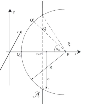
2.3 The Rayleigh-I integral for focused fields
In this Subsection, we will focus on the first version of the Rayleigh diffrac-tion integrals, the so-called Rayleigh-I intgeral. For an incident focused field, this intgeral is obtained by the substitution of Eq.(2.11) in Eq.(2.10) and, including the aberration phase Φ(x′, y′) introduced in Appendix B, we get
Ef(x, y, z;z′) =− i λ ZZ A z−z′ R2 QPRQF E0(x′, y′) exp{iΦ(x′, y′)} × exp{ik(RQP −RQF)}dx′dy′, (2.15) where Q(x′, y′, z′) again is the general point in the diffracting aperture A and (z −z′)/RQF can be recognized as an obliquity factor for the strength of the emitted secondary waves. The integral expression above neglects the diffracted near-field contribution, but for kRQP >> 1, it is sufficiently accurate if the Kirchhoff boundary conditions apply.
A direct comparison of the Rayleigh and Debye integral expressions can be carried out by transforming the Debye integral of Eq.(2.14) from an integration over the (kx, ky)-domain back to the (x′, y′)-domain in the planar diffracting apertureA. With the focal pointF located on the z-axis, the relation between the coordinates (x′, y′) and the wave vector components (kx, ky) is given by, see Fig. 2.4, kx = kz zf −z′ x′ = − k RQF x′, ky = kz zf −z′ y′ = − k RQF y′, (2.16)
F x y z=z’ Q Q’ P Q’0 R α a z Q
A
Fig. 2.4. Schematic drawing of the apertureA limiting the incident wave with its focus in the axial pointF. The possible amplitude and phase variation over the beam cross-section inAare preferably measured or calculated on the exit pupil sphere with radius R, centered in F and intersecting the z-axis in the point Q′0. In the figure, the aperture cross-section is chosen to be circular but a more
general shape can also be accommodated. with R2QF=x′2 + y′2 + (zf − z
′
)2. The Jacobian of the transformation yields
dkxdky=dx
′
dy′ k2(zf−z
′
)2/RQF4 and, withkz = kcosαQ = k(zf−z
′
)/RQF and after some rearrangement, we find the transformed Debye integral according to E(x, y, z;z′) =−i λ ZZ A zf −z ′ R3 QF E0(x ′ , y′) exp{iΦ(x′, y′)} × exp{ik·(rQP −rQF)}dx′dy′, (2.17) with the aberration function Φ of the incident wave explicitly included in the integral and the components of the vector k defined by Eq.(2.16).
Discrepancies between the Rayleigh-I and the Debye integral are found in the amplitude or obliquity factor where the difference between RQP and RQF and the difference between z and zf is neglected in the Debye expression. Another important difference is found in the pathlength exponential. The pathlength difference RQP −RQF of the Rayleigh-I integral is approximated by the scalar product s· (rQP − rQF) with s the unit vector in the propagation direction. Like for the obliquity factor above, the expressions are sufficiently accurate when P and F are close and R is very large with respect to λ. The pathlength expression in the Debye integral is exact if R → ∞ and it then corresponds
to the pathlength definition along a geometrical ray given by Hamilton in the framework of his eikonal functions [Born, Wolf (2002)]. The evaluation of the function E0(x
′
, y′) exp{iΦ(x′, y′)} can be carried out in the plane of the aperture A by measuring in A the amplitude and phase differences between the actual wave and the ideal spherical wave. The function E0exp(iΦ) carries
the information about the amplitude and phase of the bundles of rays that have been traced through the optical system. These quantities are preferably defined on the exit pupil sphere of the optical system, the sphere with radius
R, centered on F in Fig. 2.4 and truncated by the physical aperture A.
2.4 Comparison of the various diffraction integrals
A comparison of the various diffraction integrals for focused fields leads to the following order in terms of accuracy and degree of approximation
• Rayleigh-I integral
The Rayleigh-I integral according to Eq.(2.15) is the most accurate one, within the framework of scalar diffraction theory. The integral is related to the amplitude distribution in a plane. A comparable accurate integral can be obtained from Eq.(2.9), the so-called Rayleigh-II integral.
• Debye integral
The Debye integral, Eq.(2.14), yields accurate results once the distance from pupil to focal point is large (Q′0F = R → ∞) and the aperture of the cone of plane waves is sufficiently large. The angular spectrum is truncated according to the geometrical optics approximation, but this truncation has less and less influence when R increases (see [Wolf, Li (1981)] for the residual error of this integral). The functionsE0, see Eq.(2.14), accounts for a non-uniform
(complex) amplitude of the incident spherical wave.
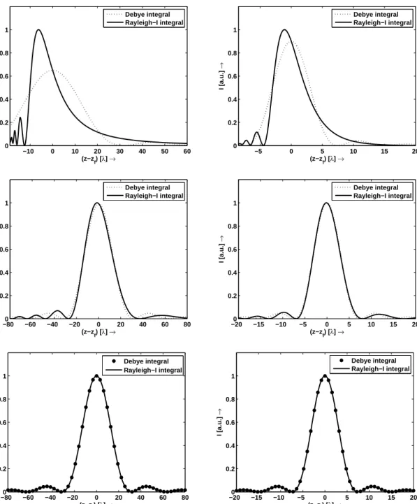
A numerical comparison of the axial intensity in the focal region according to the Rayleigh-I and the Debye integral is given in Fig. 2.5. The graphs in the upper, middle and lower row apply to increasing aperture diameters of 10λ, 100λ and 105λ, respectively. In the left column of the graphs, the numerical aperture s0 = sinαm of the focused beam in free space is 0.25, in the right column 0.50. The plotted intensity patterns, in arbitrary units, have been nor-malized with respect to the most accurate result following from the Rayleigh-I integral (solid lines). The curve following from the Debye approximation of the diffraction integral is the dotted one. The variable plotted along the horizontal axis is the defocusing (z−zf) in units of λ. The two upper graphs show that
−10 0 10 20 30 40 50 60 0 0.2 0.4 0.6 0.8 1 (z−z f) [λ] → I [a.u.] → Debye integral Rayleigh−I integral −5 0 5 10 15 20 0 0.2 0.4 0.6 0.8 1 (z−z f) [λ] → I [a.u.] → Debye integral Rayleigh−I integral −800 −60 −40 −20 0 20 40 60 80 0.2 0.4 0.6 0.8 1 (z−zf) [λ] → I [a.u.] → Debye integral Rayleigh−I integral −200 −15 −10 −5 0 5 10 15 20 0.2 0.4 0.6 0.8 1 (z−zf) [λ] → I [a.u.] → Debye integral Rayleigh−I integral −800 −60 −40 −20 0 20 40 60 80 0.2 0.4 0.6 0.8 1 (z−zf) [λ] → I [a.u.] → Debye integral Rayleigh−I integral −200 −15 −10 −5 0 5 10 15 20 0.2 0.4 0.6 0.8 1 (z−zf) [λ] → I [a.u.] → Debye integral Rayleigh−I integral
Fig. 2.5. The axial intensity in the focal region calculated according to the Rayleigh-I (solid lines) and the Debye integral expression (dotted lines). Upper row: aperture diameter 2ais 10λ. In the middle row, the aperture diameter has been increased to 100λ, in the lower row we have taken 2a= 105
λ. In the graphs on the left, the numerical aperture s0 of the focusing beam in free space is 0.25, in
the graphs on the right the value is 0.50. The intensity in arbitrary units has been normalized to the result of the Rayleigh-I integral. The defocusingz−zf has been plotted along the horizontal axis in
units of the wavelengthλof the light.
for a very small aperture diameter the difference between the Rayleigh-I and Debye integral is large. The Rayleigh-I integral result leads to a strong asym-metry with respect to the nominal focus position and the highest intensity is at an axial position closer to the aperture than the nominal focal point F. These effects are relaxed by an increase of the numerical aperture as shown by
the upper right graph. The strong intensity oscillations at the negative defocus values −20 ≤ z−zf ≤ −10 in the upper left graph correspond to axial points that are very close to the diffracting aperture itself. They can be explained by the interference effect between the wave diffracted from the circular rim of the aperture and the undiffracted focused wave, both having comparable ampli-tudes close to the aperture. The axial range beyond the intensity maximum and the focal point F does not show these deep oscillations because in this region the direct undiffracted spherical wave has, by far, the largest amplitude on axis. The effect of a higher numerical aperture is a less pronounced focus off-set of the Rayleigh-I integral; one also observes an increased fidelity of the Debye integral result regarding maximum intensity. An increase of the aper-ture diameter to 100λ makes the focus offset almost disappear, especially in the graph on the right with s0 = 0.50. The asymmetry around focus in the
position of the relative maxima is still visible, but the Debye approximation has strongly improved with respect to the upper row of graphs, also regard-ing its prediction of maximum intensity. The correspondence between both representations is increasingly better and beyond the value 2a = 500λ hardly any difference is noticeable. This is illustrated in the lower row of graphs that applies to the very large apertures encountered in practical optical systems, for instance 2a = 5 mm with λ = 0.5 µm. Here, we have plotted the De-bye approximation results as dots and these coincide extremely well with the Rayleigh-I integral results in the range of numerical apertures that are of in-terest for high-resolution applications. It is for imaging systems in this domain that the quality assessment using point-spread functions will be carried out. The lower graphs show that in this case it is fully justified to resort to the analytically more accessible Debye integral.
• Paraxial approximation of the Debye integral
The paraxial approximation to the Debye integral is allowed if the aperture shape is such that k2
z ≫ (kx2 + k2y) within the cone of integration Ω, see Eq.(2.14). The kz-factor in the nominator of the integrand is put equal to
k. The variables (kx, ky) are transformed according to kx = −k(x
′ s/R) and ky = −k(y ′ s/R) with (x ′ s, y ′
s) cartesian coordinates on the exit pupil sphere throughQ′0 with radius Rthat has its midpoint in the focal point F, located on the z-axis, see Fig. 2.4. After some manipulation and expanding the square root for kz in the pathlength exponential up to the first power we obtain Ef(x, y, z;z′)≈ − i λR2 exp{ik(z−zf)}exp ik(x 2 +y2) 2R ×
ZZ A exp − ik(z−zf) (x′2 s +y ′2 s ) 2R2 Es(x ′ s, y ′ s)× exp{iΦs(x ′ s, y ′ s)}exp − ikxx ′ s +yy ′ s R dx′sdy′s. (2.18) The amplitude function Es(x
′
s, y
′
s) and phase function exp{iΦs(x
′
s, y
′
s)}, de-scribing the departure of the complex amplitude of the focusing wave from that of a uniform spherical wave, are now defined on the exit pupil sphere where they can easily be calculated or measured.
The paraxial approximation of Eq.(2.18) is often modified to allow the use of dimensionless coordinates. The aperture coordinates are normalized with respect to the lateral dimension a of the aperture. The lateral field co-ordinates of the image point P are normalized with respect to the quantity
λR/a or λ/s0, the diffraction unit in the focal region (s0 = sinαmax = a/R is the numerical aperture of the focusing beam). The axial coordinate z is normalized with respect to the axial diffraction unit, λ/(πs2
0). With these transformations we find Ef(xn, yn, zn)≈− is20 λ exp i2(zn−zn,f) s2 0 exp ( i πλ Rs2 0 (x2n+yn2) ) × Z Z An expn−i(zn −zn,f)(x ′2 n + y ′2 n) o E(x′n, yn′ )× exp{iΦ(x′n, yn′ )}expn−i2π(xnx ′ n+yny ′ n) o dx′ndyn′ . (2.19)
Using normalized polar coordinates (ρ, θ) in the aperture and cylindrical coordinates (r, φ, f) in the focal region (origin of the normalized axial coor-dinate f is in F) yields the expression
Ef(r, φ, f)≈− is2 0 λ exp ( i2f s20 ) exp iπλr 2 Rs20 × Z Z An expn −if ρ2o E(ρ, θ) exp{iΦ(ρ, θ)} × exp{−i2πrρcos(θ −φ)}ρdρdθ, (2.20)
where the amplitude and aberration functions in cartesian coordinates now have been replaced by their analoga in polar coordinates.
2.5 The amplitude of the point-spread function produced by an optical system
The intensity distribution in the point-spread function strongly depends on the departure of the incident focusing wave from its reference shape, that of a spherical wave with a uniform amplitude. In this subsection we discuss, espe-cially for the high-numerical-aperture case, the various factors that influence the complex amplitude distribution of the focusing wave, measured in the exit pupil of the imaging system. We also discuss the various methods for repre-senting the wavefront aberration on the exit pupil sphere.
2.5.1 Amplitude distribution in the exit pupil
For the calculation of the amplitude in the focal region of an optical imaging system we need the complex amplitude distribution on the exit pupil sphere of the system. In most practical case, we are able to specify the complex amplitude distribution on the entrance pupil sphere or on the entrance pupil plane in the frequently occurring case that the object conjugate of the system is at infinity. The transfer of complex amplitude from entrance to exit pupil depends on numerous factors like diaphragm shape, reflection losses at the intermediate optical surfaces, light absorption in the lens materials, etc. These effects, particular for each optical system, can be accounted for in the complex transmission functionE(ρ, θ) exp{iΦ(ρ, θ)}. A more general aspect is the pupil imaging telling us how the complex amplitude distribution in object space is mapped to the exit pupil sphere in image space. In Fig. 2.6 we show the geometry that is relevant for this mapping process from object to image space. Several options may occur in practical systems. To study these options, we consider the intensities in an annular region of the entrance pupil and the corresponding annulus on the exit pupil sphere. The more general situation with a finite object distance and a spherical entrance pupil surface does not basically change the result. Supposing loss-free light propagation, the relation between the power flow through the annular regions of entrance pupil and exit pupil is given by
2πI0 r0dr0 = 2πp(α)I1R2sinαdα, (2.21)
where r0 = q
x2
0 +y02 is a function of α that determines the mapping effect and
the ratio I1/I0 = (fL/R)2 follows from the paraxial magnification between the exit pupil and entrance pupil (fL is the focal distance of the imaging system).
Optical system Entrance pupil Exit pupil S0 1 S P(r,φ) z αmax Q’ Q’(ρ,θ) F R x y0 0 x y x’ y’ a 0
Fig. 2.6. An incident wave is described by its complex amplitude on the entrance pupil sphere S0
(flat in this picture with the object point at infinity) and propagates from the entrance pupil through the optical system towards the exit pupil sphere S1 and to the focal region with its center in F.
The co-ordinates in object and image space are referred to by (x0, y0, z0) and (x, y, z), respectively,
with respect to the origins in object and image space. The general pointQ′ on the exit pupil sphere
is defined by means of its polar coordinates (ρ, θ) with respect to the z-axis. The aperture of the imaging pencil (diameter 2a) is given bys0 = sinαmax. The distance fromQ
′
0 toF is denoted byR
with the origin for thez′-coordinate on the exit pupil sphere chosen in Q′
0.
The function p(α) is unity on axis but can deviate from this value for α 6= 0 to account for non-paraxial behaviour of finite rays in the imaging system. The integration of Eq.(2.21) from 0 to a general aperture value given by sinα yields
r02 = fL2
α
Z
0
p(α) sinαdα. (2.22)
We consider two options
• p(α) = 1, yielding
r0 = 2fLsin(α/2) Herschel’s condition (2.23)
• p(α) = cosα, yielding
r0 = fLsinα Abbe’s sine-condition (2.24)
The two pupil imaging conditions applying to non-paraxial rays have already been proposed in the nineteenth century. They emerge as special cases in the framework of general isoplanatic imaging conditions, see [Welford (1986)]. Out-side the paraxial imaging regime, the Herschel condition favors the imaging of
axial points in front and beyond F; the Abbe sine-condition has been designed to guarantee good imaging for image points in the focal image plane through
F. The vast majority of optical systems obeys the Abbe sine condition and for this reason, in the following, we will adhere to the condition p(α) = cos(α). The function p(α) pertains to the ratio of intensities. In the case of a uniform amplitude distribution in the entrance pupil, we will thus apply the rule, with cos2α = (1 − s20ρ2), that the amplitude function on the exit pupils sphere,
E(ρ, θ), contains a factor (1−s20ρ2)1/4. This amplitude factor is often referred to as the radiometric effect. As defined before, ρ is the normalized radial co-ordinate on the exit pupil sphere.
2.5.2 Phase distribution in the exit pupil
The aberration function Φ(ρ, θ) originates from the possible aberration that is already present in the incident beam and from the aberration imparted to the beam on its traversal of the optical system. It is common practice to effectively project back the effect on the aberration of all optical surfaces and media in the system onto the exit pupil sphere, yielding the global aberration function Φ(ρ, θ) of the system. For sufficiently small aberrations, typically Φ ≤2π, this method is allowed.
The representation of the aberration function has its particular history. From the start of modern aberration theory by Seidel, see [Welford (1986)], based on a power series expansion of optical pathlength differences in an optical system, it was common practice to represent Φ as
Φ(ρ, θ) =X
aklρkcosl(θ). (2.25)
Certain combinations of k and l yield a characteristic aberration. This is more or less true for the lowest order aberration types that occur in an optical system with rotational symmetry when k + l = 4. But for higher order aberration terms, the expression of Eq.(2.25) becomes rather confusing because of the non-orthogonality of the expansion in both ρ and θ. A breakthrough in aberration theory is due to advent of the Zernike circle polynomials, see references [Zernike (1934)]-[Nijboer (1942)], and the expansion for Φ now reads
Φ(ρ, θ) = X nmR m n(ρ) n αmn,ccosmθ +αmn,ssinmθo, (2.26)
where Rmn(ρ) is the radial Zernike polynomial of radial order n and azimuthal order m with n, m ≥ 0 and n−m even. An alternative representation is
Φ(ρ, θ) = X
nmα m
n Rn|m|(ρ) exp{imθ}, (2.27)
where n ≥ 0, (n− |m|) even, and m now also assumes negative values. This latter expansion will be used and, more generally, we will also allow complex coefficients αmn so that a complex function Φ(ρ, θ) can be expanded. The re-lationship between the now equally complex coefficients αm
n,c/s and the αmn is then given by ℜ(αmn,c) =ℜ(αnm+α−nm) ℑ(αmn,c) =ℑ(αnm+α−nm) ℜ(αmn,s) =−ℑ(αmn −α−nm) ℑ(αmn,s) =ℜ(αnm−α−nm). (2.28)
Other representations of the complex amplitude on the exit pupil sphere have been proposed. We mention the expansion of the far-field using ’multi-pole waves’, see [Sheppard, T¨or¨ok (1997)]. As a function of the azimuthal and elevation angles on the exit pupil sphere, the far-field is described with the aid of spherical harmonics. The coefficients that yield the optimum far-field match are then used to propagate the multipole waves towards and beyond the focal point. The propagation as a function of the distance r is described in terms of well-behaving spherical Bessel functions of various orders. So far, the analysis has been restricted to circularly symmetric geometries with amplitude (trans-mission) variation on the exit pupil and to an infinitely distant exit pupil. But the method can be extended to more general geometries and to aberrated waves. The method is applicable not only to scalar diffraction problems but equally well to high numerical aperture systems requiring a vector diffraction treatment and can be extended to birefringent media, see [Stallinga (2004-1)]. Another representation uses the so-called Gauss-Laguerre polynomials that are orthogonal on the interval [−∞ < r < +∞] and emerge as eigenfunctions of the solution of the paraxial wave equation according to [Siegman (1986)]. They have been further studied in [Barnett, Allen (1994)] to make them suit-able for the non-paraxial case . We will not further consider this type of am-plitude and aberration representation because its Gaussian shape is not well suited for the hard-limited aperture functions that are mostly encountered in optical imaging systems. But the Gauss-Laguerre elementary solutions with
azimuthal order number m 6= 0 are well suited to represent a phase departure of the pupil function that shows a so-called helical phase profile with a phase jump of 2mπ. This is interesting when discussing optical beams with orbital angular momentum, see for instance [Beijersbergen, Coerwinkel, Kristensen, Woerdman (1994)]. However, using the Zernike polynomial representation of Eq.(2.27) with the exponential azimuthal dependence, it is equally well possible to represent helical phase profiles by selecting a single nonzero αmn-coefficient instead of an automatic combination of αnm and α−nm.
Using the appropriate expressions for the amplitude and aberration function on the exit pupil sphere we are now able to evaluate Eq.(2.20) and to obtain the amplitude of the scalar point-spread function in the paraxial approximation. It is possible to extend the scalar integral of Eq.(2.20) beyond the paraxial domain by incorporating the defocus exponential of Eq.(2.14) according to
exp{ikz(z −zf)} = exp{ik v u u t1− k 2 x+ k2y k2 (z −zf)}. (2.29)
With the same coordinate transformation as used in deriving Eq.(2.18) and switching to the normalized polar coordinates (ρ, θ) on the exit pupil sphere, we obtain
exp{ikz(z −zf)} = exp{ik
q
1−s2
0ρ2 (z −zf)}. (2.30)
The axial coordinate z−zf is normalized in the high numerical aperture case according to z−zf = − f ku0 , (2.31) with u0 = 1 − q
1−s20 and one then finds the final expression for the
high-numerical-aperture defocus exponential, viz.
exp{ikz(z −zf)} = exp " −i f u0 # exp ( i f u0 1−q1−s20ρ2 ) . (2.32)
The scalar integral for high-numerical-aperture then reads
Ef(r, φ, f)≈− is20 λ exp ( −if u0 ) exp iπλr 2 Rs2 0 ×
Z Z An exp if 1−q1−s20ρ2 u0 E(ρ, θ) exp{iΦ(ρ, θ)} × exp{−i2πrρcos(θ−φ)}ρdρdθ, (2.33)
where the complex amplitude angular spectrum functionE(ρ, θ) exp{iΦ(ρ, θ)} is again evaluated on the exit pupil sphere using the data from ray tracing or other propagation methods of the wave through the optical system. In several instances in the literature, the minus sign in the exponential with the factor cos(θ−φ) in Eq.(2.33) has also been suppressed. This means that the results apply to an azimuth shift of π for the axis φ = 0 in image space. In Section 3 and further of this chapter, we will adhere to this latter sign convention. The integral above is an improvement with respect to the paraxial approximation, beyond an aperture of 0.60, at the condition that polarization effects are not dominating. In practice, this might be the case when the optical system is illuminated with effectively unpolarized or ’natural’ light.
2.5.3 The high-numerical-aperture vector point-spread function
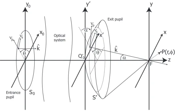
The extension of the point-spread function analysis to the vector compo-nents of the electrical and magnetic fields was first carried out in [Ignatowsky (1919)]. In a series of three papers he analyzed the electromagnetic field in the focus of a parabolic mirror and in the focus of a general imaging system. He also analyzed the amplitude conversion from entrance to exit pupil fol-lowing from the various pupil imaging conditions, see Eqs.(2.23)-(2.24). The subject was reformulated and cast in the form of a generalized Debye integral by [Wolf (1959)] and [Richards, Wolf (1959)], applied to an optical system that is illuminated by a parallel beam from infinity with the optimum focus of the point-spread function in the geometrical focal point F. The Debye integral is used to solve the diffraction problem for each cartesian vector component of the fields. The vector components of the fields on the exit pupil sphere are obtained using the condition of Abbe for the mapping of the field components from the entrance pupil to the exit pupil (aplanatic imaging). From the geom-etry of the problem, see Fig. 2.7, one easily derives the required unit vectors in image space that are associated with the s- and p-polarization components
Optical system Entrance pupil Exit pupil S0 S’ P(r,φ) z α F x y0 0 x y x’ y’ k ν νp s ^ θ θ α ν νp s k ^ Q’0
Fig. 2.7. Definiton of the orthogonal unit vector sets (νs, νp,ˆk)in entrance and exit pupil that are used
to describe the components of the electromagnetic field vectors in the image space. The azimuthal plane defined by the angle θ is the plane of incidence. The origin for the exit pupil coordinates is chosen inQ′0 with Qa general point on the exit pupil sphere.
and the unit propagation vector
νp = cosθcosα sinθcosα sinα νs = sinθ −cosθ 0 ˆ k = −cosθsinα −sinθsinα cosα . (2.34)
The incident field is specified in terms of the linearly polarized electric compo-nents along thex0- andy0-axis in the entrance pupil according toE= a0ˆx+b0ˆy,
with a0 and b0 complex numbers to allow for an arbitrary state of polarization
of the incident beam. The p- and s-polarization components of the field on the exit pupil sphere are now given by
Ep∝ {a0cosθ+b0sinθ} cosθcosα sinθcosα sinα ,
Es∝ {a0sinθ−b0cosθ} sinθ −cosθ 0 . (2.35)
Thex-, y- and z-components of the field on the exit pupil sphere is obtained by evaluating the scalar products with the cartesian unit vectors and this yields
Es,x= fLk 1/2 z 2Rk1/2 " a0 ( 1 + kz k −cos 2θ 1− kz k !) −b0sin 2θ 1− kz k !# Es,y= fLkz1/2 2Rk1/2 " −a0sin 2θ 1− kz k ! +b0 ( 1 + kz k + cos 2θ 1− kz k !)# Es,z= fLkrkz1/2 Rk3/2 (a0cosθ+b0sinθ) , (2.36) with kr = k q 1−k2
z/k2 and where we have included the amplitude mapping factor from the entrance to the exit pupil (see Subsection 2.5.1). The unit vector that points in the direction of the magnetic field is given by hˆ=kˆ×ˆe, yielding ˆhp = (cosαcosθ,cosαsinθ,sinα) and ˆhs = (−sinθ,cosθ,0). The cartesian components of the magnetic induction are then given by
Bs,x= nrfLkz1/2 2cRk1/2 " −a0sin 2θ 1− kz k ! −b0 ( 1 + kz k −cos 2θ 1− kz k !)# Bs,y= nrfLkz1/2 2cRk1/2 " a0 ( 1 + kz k + cos 2θ 1− kz k !) +b0sin 2θ 1− kz k !# Bs,z=nrfLkrk 1/2 z cRk3/2 (a0sinθ−b0cosθ) , (2.37)
with nr the refractive index of the image space.
With the expressions for the electric and magnetic field components in terms of the wave vector componentskx and ky, the Debye integral of Eq.(2.14), with
xf = yf = 0, yields for the field components in the focal region near F
E(x, y, z) =−i 2π ZZ Ω Es(−kx,−ky) kz exp{i[kxx+ kyy +kz(z−zf)]}dkxdky B(x, y, z) =−i 2π ZZ Ω Bs(−kx,−ky) kz exp{i[kxx+kyy +kz(z−zf)]}dkxdky, (2.38)
with P(x, y, z) the coordinates of the considered point in the focal region. Using the more appropriate normalized cylindrical coordinates (ρ, θ) on the exit pupil sphere and (r, φ) in the focal region, we obtain
E(r, φ, f) =−is 2 0 λ exp −if u0 ! ZZ C Es(ρ, θ+π) (1−s20ρ2)1/2 × exp ( if u0 h 1−(1−s20ρ2)1/2i ) exp{i2πrρcos(θ−φ)}ρdρdθ, (2.39) with C the scaled integration area on the exit pupil sphere (in a standard situation equal to the unit circle); a comparable expression holds for the B -field components. In arriving at Eq.(2.39), we used Eq.(2.31) and the following coordinate transformations and normalizations,
kx=krcosθ = ρkr,maxcosθ, kr,max = ks0,
ky=ρkr,maxsinθ,
kz= (k2 −k2x−ky2)1/2 = k(1−s20ρ2)1/2,
r=ks0
2π (x
2 +y2)1/2, (2.40)
with the field strength function Es, originally defined as a function of the wave vector components (kx, ky), now to be measured as a function of the normalized radial aperture coordinate ρ on the exit pupil sphere and the azimuthal coor-dinate θ+π. The position on the exit pupil sphere is obtained from Eq.(2.13) using x = xf −(kx/k)R, y = yf −(ky/k)R, leading to real space coordinates of (x = −ρacosθ, y = −ρasinθ), in normalized polar coordinates (ρ, θ +π); note that this latter phase off-set of π is missing in [Wolf (1959)].
2.6 Analytic expressions for the point-spread function in the focal region (scalar case)
The first analytic solution of the aberration-free point-spread function inte-gral of Eq.(2.20) goes back to [Lommel (1885)] and is treated in detail in [Born, Wolf (2002)]. The solution for the aberrated case has been studied by vari-ous authors, see [Conrady (1919)], [Steward (1925)], [Picht (1925)], [Richter (1925)]. A more systematic analysis of the influence of aberrations on the point-spread function became possible after the introduction of the Zernike polynomials to describe the wavefront aberration, see [Zernike (1934)],
[Ni-jboer (1942)], [Zernike, Ni[Ni-jboer (1949)]. Considering the integral of Eq.(2.20) for a circular aperture (unit circle), we first substitute the Zernike expansion for the aberration function and use the approximation exp(iΦ) ≈ 1 +iΦ for small values of Φ, typically Φ ≤1. We thus obtain
Ef(r, φ, f)≈ 2π Z 0 1 Z 0 expnif ρ2oE(ρ, θ){1 +iX nmα m nRn|m|(ρ) exp(imθ)} × exp{i2πrρcos(θ−φ)}ρdρdθ. (2.41)
Carrying out the integration over θ and using the property
2π
Z
0
exp(imθ) exp{i2πrρcos(θ−φ)}dθ = 2πimJm(2πrρ) exp(imφ), (2.42)
we get the expression originally derived by Nijboer in his thesis [Nijboer (1942)], Ef(r, φ, f)≈2πi 1 Z 0 expnif ρ2oE(ρ, θ)× ( [(1 +α00)J0(2πrρ)] + X nmi m+1αm nR|nm|(ρ)Jm(2πrρ) exp(imφ) ) ρdρ, (2.43)
where the summation now has to be carried out over all possible (n, m)-values with the exception of m = n = 0. As usual, the function Jm(x) denotes the Bessel function of the first kind of order m. We remark here that, instead of expanding the function Φ itself using the α-coefficients, it is also possible to expand the complete pupil function E(ρ, θ) exp{iΦ(ρ, θ)} in terms of Zernike polynomials, as it was first proposed in [Kintner, Sillitto (1976)].
A basic result from aberration theory, initially derived by Nijboer, is the following 1 Z 0 R|nm|(ρ)Jm(2πrρ)ρdρ = (−1) n−|m| 2 Jn+1(2πr) 2πr . (2.44)
In the perfectly focused case and forE(ρ, θ) ≡1, the integral above is sufficient to analytically calculate the amplitude Ef with zn = 0 in Eq.(2.43). However, in the defocused case, the analysis becomes more complicated and Bauer’s formula has been used by Nijboer to obtain a workable expression [Nijboer
(1942)], exp(if ρ2) = exp(if /2) X∞ n=0 (2n+ 1)in jn f 2 ! R02n(ρ). (2.45)
The spherical Bessel function jk(x) of the first kind is defined by
jk(x) =
s π
2x Jk+12(x) , k = 0,1, ... , (2.46)
see [Born, Wolf (2002)], Ch. 9, and [Abramowitz (1970)], Ch. 10. The extra radial Zernike polynomials that result from the expansion of the quadratic defocus exponential can be treated by formulae that express the product of two Zernike polynomials into a series of Zernike polynomials with differing upper or lower indices. This approach has been discussed by Nijboer. In practice, his solution allows to solve the problem of the defocused aberrated point-spread function for modest defocus values, for instance|f| < π/2. When trying to reconstruct aberrations from defocused intensity distributions, numerically reliable expressions for the intensity of the out-of-focus point-spread function are required over a larger range of f-values. The work described in Nijboer’s thesis does not yet provide such results. It should be added that, even if these results would have been available, the lack of advanced computational means would have prohibited any further activity in this direction at that time.
2.6.1 Analytic solution for the general defocused case
A semi-analytic solution of the aberrated diffraction integral in the defocused case was presented in [Janssen (2002)] and its application and convergence domain was studied in [Braat, Dirksen, Janssen (2002)]. The basic integral occurring in, for instance, Eq.(2.43) reads
Vnm(r, f) =
1 Z
0
expnif ρ2oR|nm|(ρ)Jm(2πrρ)ρdρ , (2.47)
and its solution is found to be an infinite Bessel function series according to
Vnm(r, f) =ǫmexp [if] ∞ X l=1 (−2if)l−1 p X j=0 vlj J|m|+l+2j(2πr) l(2πr)l . (2.48)
In Eq.(2.48) we have to choose ǫm = −1 for odd m < 0 and ǫm = 1 otherwise. The function Vm
n (r, f) provides us with the analytic solution of the integrals that occur in the general expression of Ef in Eq.(2.43) and they are associated with a typical Zernike aberration of radial order n and azimuthal order m. To obtain the total expression for Ef, it is just required to insert the appropriate azimuthal dependence. Denoting
p= n− |m|
2 , q =
n+|m|
2 , (2.49)
the coefficients vlj in Eq.(2.48) are given as
vlj= (−1)p(|m|+l + 2j)× | m|+j +l−1 l−1 j+l −1 l −1 l−1 p−j q +l+j l , (2.50)
for l = 1,2, . . . , j = 0,1, . . . , p. The binomial coefficients are defined by
n m = n(n−1)· · ·(n−m+ 1) m! (2.51)
with the remark that any binomial with n < m is put equal to zero. To illustrate the accuracy of the series expansion, it can be shown that an absolute accuracy of 10−6 requires a number lmax of terms in the summation that is given by lmax = |3f|+ 5. With this number of terms and a range |f| ≤ 2π, the amplitude in the focal region of interest of well-corrected optical imaging systems can be calculated with ample precision.
Some special cases for the scalar amplitude Ef of Eq.(2.43) can be directly derived using the results of Eqs.(2.48)-(2.51).
• Nijboer’s in-focus result of Eq.(2.44) is obtained for the special case of Eq.(2.48) with f=0, where the summation over l is now restricted to the term with l = 1 and the coefficient v1j is identical (−1)(n−|m|)/2, regardless the value of j.
• The special case withm = n = 0 corresponds to the aberration-free situation that should yield the result originally obtained by Lommel. Referring to Eq.(2.47), Lommel’s solution reads, see [Born, Wolf (2002)],
V00(r, f) = 1 Z 0 expnif ρ2oJ0(2πrρ)ρdρ = C(r,2f) +iS(r,2f) 2 , (2.52)
with the functions C and S given by C(r, f) =cos(f /2) f /2 U1(r, f) + sin(f /2) f /2 U2(r, f) , S(r, f) =sin(f /2) f /2 U1(r, f)− cos(f /2) f /2 U2(r, f), (2.53)
with the general Lommel-function Un(r, f) defined by
Un(r, f) = ∞ X s=0 (−i)2s f 2πr !2s+n J2s+n(2πr) . (2.54)
The substitution of Lommel’s results in Eq.(2.52) leads, after some rear-rangement, to the expression
V00(r, f) = exp(if)X∞
l=1
(−2if)l−1Jl(2πr)
(2πr)l . (2.55)
It is seen that this compact expression of Lommel’s result is equivalent to the special case with n = m = 0 of Eq.(2.48) once we have substituted the value vl0 = l.
• The on-axis amplitude distribution is obtained from Eq.(2.43) with r = 0. If we limit ourselves to circularly symmetric aberrations with m = 0 and use Bauer’s formula of Eq.(2.45) for the defocus exponential, the integral over
ρ is easily evaluated with the aid of the properties of the inner products of the radial Zernike polynomials and we find
Ef(0,0, f) ≈ iπ exp(if /2) j0(f /2) + ∞ X n=0 inα02njn(f /2) . (2.56)
In the aberration-free case, the axial dependence is given by the spherical Bessel function of zero order. With the identity j0(x) = sin(x)/x, we find
the Lommel result above.
Another analytic result from [Janssen (2002)] is related to diffraction inte-grals of the type
Tnm(r, f) =
1 Z
0
expnif ρ2oρnJm(2πrρ)ρdρ . (2.57)
These integrals with a ρ-monomial in the integrand can be considered to be the building blocks for more general integrals containing a polynomial like a Zernike polynomial. Of course, they are also useful in the context of the
aberration representation according to Seidel. The Bessel series solution of this type of integral is given by
Tnm(r, f) = ǫmexp [if] ∞ X l=1 (−2if)l−1 p X j=0 slj J|m|+l+2j(2πr) (2πr)l . (2.58)
In Eq.(2.58) we again choose ǫm = −1 for odd m < 0 and ǫm = 1 otherwise. The coefficients slj are given by
slj = (−1)j |m|+l + 2j q + 1 p j | m|+j +l−1 l−1 q +l +j q + 1 , (2.59)
for the same ranges as in the case of vlj: l = 1,2, . . . , j = 0,1, . . . , p.
In the case of circularly symmetric aberrations a different expansion of the diffraction integral has been proposed in [Cao (2003)] and it produces analytic expressions for the functions T20p(r, f) defined above. The exponential factor exp(if ρ2) is written as a Taylor series inf and this gives rise to the appearance of the so-called Jinc-functions with index n according to
Jincn(r) = 1 (2πr)2n+2 2πr Z 0 x2n+1J0(x)dx, (2.60)
for which Bessel series expansions are given. A convergence problem is present with respect to the power series expansion in f and the condition |f| ≤ 15 should be respected to obtain an accuracy of 10−3 in amplitude, 10−6 in inten-sity.
The analytic expressions for the general functions Vnm(r, f) andTnm(r, f) are composed of a Bessel function expansion with the argument 2πr and a power series expansion with respect to f. The latter series expansion, especially for the V-functions, gives rise to numerical convergence problems once the value of |f| is larger than, say, 5π and an accuracy of 10−8 in amplitude can not be achieved for largerf-values. A drastic improvement in accuracy is obtained once the power series expansion inf can somehow be replaced by a more stable expression. To this goal, we use Bauer’s expansion and write the exponential exp(if ρ2) according to Eq.(2.45). Using this in the expression for Vnm(r, f), we find Vnm(r, f) = exp(1 2if) ∞ X k=0 (2k+ 1)ikjk(f /2) ×
1 Z
0
R02k(ρ)Rn|m|(ρ)Jm(2πrρ)ρ dρ . (2.61)
To proceed further, a general expression is needed that writes the product of a radially symmetric Zernike polynomialR02k(ρ) and a general polynomial Rmn(ρ) as a series of Zernike polynomials according to
R02kR||mm||+2p = X
l
wklR||mm||+2l . (2.62)
In [Janssen, Braat, Dirksen (2004)], explicit expressions have been given for the coefficientswkl and the range of the summation index l (see also Appendix C). A numerical implementation of these results has shown that |f|-values as large as 1000 can be dealt with. To illustrate the kind of intensity distributions that can be numerically handled by the analysis according to Eqs.(2.61)-(2.62), we show in Fig. 2.8 cross-sections of strongly defocused intensity distributions. In the left figure, a contour map is shown of an axial cross-section of a focal
−5 0 5 −15 −10 −5 0 X−axis [µm] Focus [ µ m] Bessel, λ = 0.248 NA = 0.6, σ = 0 −150 −10 −5 0 0.2 0.4 0.6 0.8 1 Focus [um] Intensity (x,y)=0
Fig. 2.8. Axial cross-section of a defocused intensity distribution (f=23) caused by the presence of a Fresnel zone plate in the planez=0. The beam shows some circularly symmetric aberration that becomes visible in the figure on the right in which the axial intensity has been plotted. The numerical aperture is 0.60, the wavelength amounts toλ=248 nm.
intensity distribution that is off-set by approximately 15 focal depths from its nominal focal setting. The intensity distribution has been produced by means of a Fresnel zone lens and is affected by spherical aberration. In the right fig-ure, we show the axial intensity distribution that shows an asymmetry around focus due to this residual aberration of the focusing beam. Figure 2.9 produces a picture of the measured intensity distribution in a strongly defocused image plane (f ≈ 75). A typical Fresnel diffraction pattern is observed. Some spuri-ous structure is visible due to light scattering at imperfections on the optical
Fig. 2.9. Measured intensity distribution in a strongly defocused image plane. The value of f is approximately 75. Note that the axial intensity corresponds to a minimum due to the presence of an even number of Fresnel zones in the aperture as seen from the defocused position.
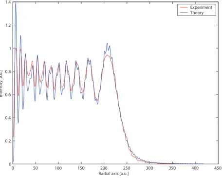
0 50 100 150 200 250 300 350 400 450 0 0.2 0.4 0.6 0.8 1 1.2 1.4 Figure − 6
Radial axis [a.u.]
Intensity [a.u.]
Experiment Theory
Fig. 2.10. Comparison of a measured intensity distribution and the best-fit calculated intensity dis-tribution. In this case the value off is 75 radians. The measured intensity shows a less pronounced modulation than the calculated distribution which may be attributed to some scattered background light and to a diaphragm rim that is not perfectly spherical.
surfaces in the experimental set-up. The number of luminous rings NF in the Fresnel diffraction pattern is approximately given by NF = (f −π)/2π.
In Fig. 2.10 we show a radial cross-section of such a defocused intensity distribution, from the central position on axis up to the geometrical shadow region. It is interesting to note that part of the fine structure in the fringes, predicted by the calculations, is also visible in the measured distribution, de-spite the high sensitivity of the measured intensity to spurious coherent light