INVENTORY COST CONSEQUENCES OF VARIABILITY DEMAND PROCESS WITHIN A MULTI-ECHELON SUPPLY CHAIN

INVENTORY COST CONSEQUENCES OF VARIABILITY DEMAND

PROCESS WITHIN A MULTI-ECHELON SUPPLY CHAIN

Francisco Campuzano Bolarín Technical University of Cartagena Departamento de Economía de la Empresa

Campus Muralla del Mar 30201 Cartagena Spain E-mail: francisco.campuzano@upct.es Andrej Lisec Univesity of Maribor Faculty of Logistics Hočevarjev trg 1 8271 Krško Slovenia E-mail: andrej.lisec@uni-mb.si

Francisco Cruz Lario Esteban Technical University of Valencia

Departamento de Organización de Empresas Economía financiera y contabilidad Camino de Vera s/n 46022 Valencia Spain E-mail: fclario@omp.upv.es ___________________________________________________________________________ Abstract

The bullwhip effect (Lee et al, 1997a) is a known supply chain phenomenon where small variations in end item demand create oscillations that amplify throughout the chain. Different price elasticity of demand influence different changes of demand when prices of items are changing on the time horizon. The variance of the orders at the end user placed on suppliers or on manufacturer increases with the orders flow upstream in the logistics chain. This creates harmful consequences in inventory levels and all kind of inventory costs that may affect added value of activities along the logistics chain and finally affect Net Present Value of all activities in the chain.

Traditional model of dynamic supply chain structures is used for this particular study, based on the seminal work of Forrester Diagrams (Forrester 1961). Simulation platform for supply chain management at stochastic demand developed by Campuzano (2006) has been used. VENSIM Simulation Software was previously used for developing these supply chain dynamic models. In the development platform generalised supply chain models are constructed graphically and also analytically. Our study here is to get a dipper insight into the processes in a logistics chain, measuring the inventory cost consequences due to variability demand amplification.

1. Introduction

A supply chain is the set of structures and processes an organization uses to deliver an output to a customer. The output can be a physical product such as an automobile, the provision of a key resource such as skilled labor, or an intangible output such as a service or product design (Sterman, 2000). A supply chain consists of the stock and flow structures for the acquisition of the inputs to the process and the management policies governing the various flows.

Each of these processes features a number of clearly defined characteristics, which represent a wide range of topics to be investigated. Research on supply chains makes an attractive field of study, offering numerous approach roads to organisational integration processes. Some of the problems regarded as most important, which canalise any research project in the area of supply chains, are those related to demand variability and demand distortion throughout the Supply Chain. Forrester (1958) analysed Supply Chain and the different levels existing in it, as well as the participant companies and the role played by each of them inside the chain as a global group, and observed that a small fluctuation in a customer’s demand was magnified as it flowed through the processes of distribution, production and provisioning. This effect was identified and also studied by Burbidge (1991) and it is known as the Forrester Effect. That amplification owed itself, according to Forrester, to the problems derived from the existence of delivery times ("non zero lead times"), and the inaccuracy of forecasts carried out by the different members of the chain in the face of the variability of the demand received.

Most of the research on the demand amplification has focused on demonstrating its existence, identifying its possible causes, and developing methods for reducing it. Lee et al. (1997a) identified five main causes of amplification: wrong methods of demand forecasting, supply shortage anticipation, batch ordering and price variation. Demand amplification occurs mostly because of finite perturbations in final demand and in lead time all along the supply chain, which is always anticipated and in interaction with other causes. By his seminal work “Industrial Dynamics, A Major Breakthrough for Decision Makers” in 1958, Jay Forrester is viewed as the pioneer of the modern-day supply chain management. His work on the demand amplification as studied via systems dynamics simulation has explored these supply chain phenomena from many viewpoints. How the industry is facing this phenomenon is broadly studied by Lee et all (1997a), where some considerations of the bullwhip effect in supply chains are presented in details, too. Our study has also been motivated by many other production-distribution considerations about bullwhip effect in the supply chain perturbations, such as those given by Lee et al (1997a), and especially the results of Disney (2001, 2002, 2003a, 2003b) and other researchers of this phenomenon from Cardiff Business School.

The objective of this work is to study the long term cost consequences of the Bullwhip effect within a generic multi–echelon supply chain. The behaviour of the generic system under study is analyzed through a simulation model based on the principles of the system dynamics methodology. The simulation model proposed by Campuzano (2006) provides an experimental tool, which can be used to evaluate alternative long term decisions such as replenishment orders, capacity planning policies, or even inter-organizational strategies (“what-if” analysis), as this methodology allows studying the interdependences among every echelon modelled.

2. Measuring the bullwhip effect

An integrated supply chain includes the purchasing of raw materials, the manufacturing with assembly or sometimes also disassembly, and the distribution and repackaging of produced goods sent to the final clients. Various operating stages in the logistic chain (nodes of the chain) can be represented by a simple model of some material-transformations or location-transformations processing cells (and arcs). In each processing cell, a value is added and some costs are incurred. At each processing cell there is a supply and a demand and often both are stochastic by nature.

Price variations or the Promotion Effect and many other actions in a supply chain refer to the practice of offering products at reduced prices to stimulate demand. Assuming an elastic demand, this creates temporary increases in demand rates where customers take advantage of this opportunity and forward buy or “stock up”. However this has serious impacts on the dynamics of the supply chain and added value especially when a certain security level of supply is prescribed.

Inventories are insurance against the risk of shortage of goods in each cell of the logistic chain. They are limited by the capacity of each processing node of the chain and transportation capability of input and output flows.

Ordering goods (input flow) in distribution centres can be studied as a multi-period dynamic problem. The demand (output flow) during each period has to be considered as a stochastic variable. The distribution of this variable is often described with a certain probability function which is here normal.

The intensity variation of flows of items in supply chains influence transportation costs and costs of activities in logistic nodes and consequently the net present value (NPV) of all activities that have to be performed in such logistic networks.

As mentioned above, bullwhip effect refers to the scenario where the orders to the supplier tend to have larger fluctuations than sales to the buyer and the distortion propagates up a supply chain in an amplified form. As distortion creates additional costs, the indicators or measures of bullwhip are supposed to be in correlation with costs or added value.

Our study was based on the production and inventory control results, especially on the variability trade off study, presented by Dejonckheere et al. (2003), a control theoretic approach to measuring and avoiding the bullwhip effect, presented by these authors, and the study of the impact of information enrichment on the bullwhip effect in supply chains - a control engineering perspective by Dejonckheere et al. (2004), where some measures have been introduced.

The amplification upstream the supply chain can be measured through the variance of demand along the supply chain. The variance of a set of data is defined as the square of the standard deviation and is thus given by s2 for estimation of population varianceσ2. Lee at al.(1997b) suggested the changes of variance in demand σ2upstream as the measure of bullwhip effect. It is a good measure only when the units of flow are not changing along the chain, which is not the case in many logistics cases. In the recent literature by Chen et al. (2000), it is suggested that to avoid this problem bullwhip effect should be measured by changing the ratio of σ2 µ upstream of supply chain, but again it does not help to avoid the effect of changing unit measure. Chen et

al. (2000) suggested that its measure could be the ratio of these parameters between input and output flows at each activity cell in a supply chain, when only one stage is considered, or the ratio of these parameters between final demand and first stage of manufacturing when total supply chain is to be evaluated (Equation 1).

(1) O: Orders

D: Demand

On the other hand Disney and Towill (2003b) propose that the last variance ratio measure can easily be applied to quantify fluctuations in net inventory as shown in Equation 2.

2 2

/

/

NSAmp

σ

µ

σ

µ

=

The System Dynamics methodology (SD) is a modelling and simulation technique specifically designed for long-term, dynamic management problems. It focuses on understanding how the physical processes, information flows and managerial policies interact so as to create the dynamicsof the variables of interest. The totality of the relationships between these components defines the “structure” of the system. Hence, it is said that the “structure” of the system, operating over time, generates its “dynamic behaviour patterns”. It is most crucial in System Dynamics that the model structure providesa valid description of the real processes. The typical purpose of a System Dynamics study is to understand how andwhy the dynamics of concern are generated and then search for policies to further improve the systemperformance. Policies refer to the long-term, macro-level decision rules used by upper management. System Dynamics

differs significantly from a traditional simulation method, such as discrete-event simulation where the most important modelling issue is a point-by-point match between the model behaviour and the real behaviour, i.e. an accurate forecast. Rather, for a System Dynamics – SD model it is important to produce the major “dynamic patterns” of concern (such as exponential growth, collapse, asymptotic growth, S-shaped growth, damping or expanding oscillations) (Vlachos et al. 2007). Therefore, the purpose of our model would not be to predict what the total

supply chain profit level would be each week for the years to come, but to reveal under what conditions the total profit would be higher, if and when it would be negative, if and how it can be controlled (Sterman 2000).

The structure of a system in SD methodology is exhibited by causal loop (influence) diagrams; a causal loop diagram captures the major feedback mechanisms—the negative feedback loops (balancing) or the positive feedback (reinforcing) loops. While a negative feedback loop exhibits a goal-seeking behaviour, i.e., after a disturbance, the system seeks to return to an equilibrium situation, in a positive feedback loop, an initial disturbance leads to further change, suggesting the presence of an unstable equilibrium. Causal loop diagrams play two important roles in SD.

2 2 2 2 / / D O D D O O Bullwhip σ σ µ σ µ σ = =

First, they serve as preliminary sketches of causal hypotheses during model development, and second, they can simplify the representation of a model. The structure of a dynamic system model contains the stock (state) and flow (rate) variables. Stock variables are the accumulations (i.e., inventories) within the system, while flow variables represent the flows in the system (i.e., order rate), which are the by-products of the decision-making process. Stock-flow diagrams represent the model structure and the interrelationships among the variables. The mathematical mapping of a SD stock-flow diagram occurs through a system of differential equations, which is numerically solved with the help of a simulation. Nowadays, high-level graphical simulation programs—such as Powersim, Stella, Vensim and i-think—support the analysis and study of these systems.

4. Problem and model construction

The main characteristics of the model used for this research are summarized in the next points:

- We have considered a four stage supply chain system consisting of identical agents, where each agent orders products only from its upper stage. These are Customer, Retailer, Wholesaler and Manufacturer.

- An agent ships goods immediately upon receiving the order if there is sufficient amount of on hand inventory.

- Orders may be partially fulfilled (every order to be delivered includes actual demand and backlogged orders- if there exist), and unfulfilled orders are backlogged.

- Shipped goods arrive with a transit lead-time of goods and they are also retarded because of information lead time.

- Last stage (manufacturer) receives raw materials from an infinite source and manufacture finished goods under capacity constraints.

The first step for developing the model was the creation of the causal loops which integrate the key factors of the system and put the relations on the links between pair of them. It is expected that the differences between bullwhip indicators are the highest in the case of the traditional supply chain. Other structures are given to reduce bullwhip effect.

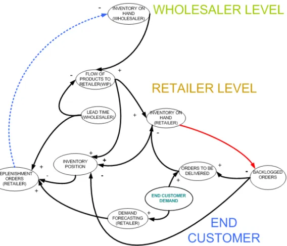
Figure 2: The causal loop frequently occurring in real cases at distribution part of the traditional supply chain. Often, its production part has varied MRP assembly or arbores cent structures. Source: Campuzano (2006) © UPCT RPI 08/2007/392

Figure 2 presents the stock and flow structure for a multi-echelon supply chain system in its corresponding causal loop diagram. The arrows represent the relations among variables. The direction of the influence lines displays the direction of the effect. Signs ‘‘+’’ or ‘‘–’’ at the upper end of the influence lines indicate the type of effect. When the sign is ‘‘+’’, the variables change in the same direction; otherwise they change in the opposite one.

5. The decision rule

The ordering policy we have chosen for our analysis is a generalized Order-Up-To policy. In any order-up-to policy, ordering decisions are as follows:

t t

O =S −inventoryposition (3)

The order quantity is equal to S_t, reduced for inventory state as:

Inventory position= Inventory on hand-backlogged orders+orders placed but not yet received.

where Ot is the ordering decision made at the end of period t,St is the order-up-to level used in

received), and net stock equals inventory on hand minus backlog. The order-up-to level is updated every period according to:

L t L t t D k S = ˆ + σˆ (4)

Where S_t is equal to the estimate mean of demand L t D ∧ over L periods ( L t t D D L ∧ ∧ = ⋅ ) increased for prescribed service level with buffer stocks, L

t

σ is an estimation of the standard deviation over L periods, and k is fill rate factor which depend on demand distribution (here it is supposed to be Normally distributed).

The policy is needed where net present value of all activities in the value chain is optimal. The ordering policy depends on demand, which is stochastic and react on price policy.

6. Numerical Investigation

In this section it is demonstrated the application of the developed methodology using a numerical example and discuss few interest insights that are obtained.

We will considerate a Traditional supply chain with four echelons, that is customer, retailer, wholesaler and manufacturer. The initial values for the main parameters of that supply chain were randomly selected:

- The demand pattern follows a normal distribution

- The initial inventory for every echelon is 100 units

- Manufacturer capacity : 160 units/per day

- Lead time for wholesaler is 3 days and for the manufacturer is 2 days. Lead times are supposed to be constant except in case of stock out

- Manufacturing process takes 2 days

- Fill rate factor for every echelon is two days

- Exponential smoothing forecasting process (α=2)

- The inventory cost were fixed as follows: o Holding cost : 0,5 euros unit/period o Stock out cost: 1 Euro/per stock-out o Order cost : 0,5 euros/order

365 periods were simulated. It is observed enough as the system reached a stable state.

6.1 Simulation results

Next Figure shows (illustration 3) the variability of the orders sent at every echelon regarding to Demand signal.

Figure 3: Variability of the orders sent at every echelon regarding to Demand signal

Next Figure shows the bullwhip effect at every echelon.

Figure 4: Bullwhip effect at every echelon

Next illustration (illustration 5) shows NSAmp at every echelon.

80 60 40 20 0 0 5 10 15 20 25 30 35 40 45 50 55 60 65 70 Time (Day) Demand Retailer Wholesaler Manufacturer 80 60 40 20 0 0 5 10 15 20 25 30 35 40 45 50 55 60 65 70 Time (Day) Demand Retailer Wholesaler Manufacturer Demand Retailer Wholesaler Manufacturer 60 45 30 15 0 0 73 146 219 292 365 Time (Day) Retailer Wholesaler Manufacturer 60 45 30 15 0 0 73 146 219 292 365 Time (Day) Retailer Wholesaler Manufacturer Retailer Wholesaler Manufacturer UNITS

Figure 5: NSAmp at every echelon

Last Figures are showing how the demand variability increases upstream the supply chain. This variability arises some problems caused by the interdependences of every echelon within the supply chain. The increment in the demand variability will produce replenishment orders with high variable sizes, what will affect the forecast process accuracy at every echelon. Therefore the inventory levels at every echelon will have a high variability too, and sometimes will not be able to face demand peaks, what will produce stock out periods. That variability will be reflected in high holding cost (inventory excess) and high stock out cost (no inventory available to satisfy replenishment orders).

Next Figure shows the fill rates reached at every level. The retailer has the lower fill rate as suffers the variable lead times at the upstream members (wholesaler and manufacturer) caused by stock-out periods at these levels.

Figure 6: Fill rates at every echelon 100 75 50 25 0 1 53 105 157 209 261 313 365 Time (Day) Retailer Wholesaler Manufacturer 100 75 50 25 0 1 53 105 157 209 261 313 365 Time (Day) Retailer Wholesaler Manufacturer Retailer Wholesaler Manufacturer 60 45 30 15 0 1 27 53 79 105 131 157 183 209 235 261 287 313 339 365 Time (Day) Retailer Wholesaler Manufacturer 60 45 30 15 0 1 27 53 79 105 131 157 183 209 235 261 287 313 339 365 Time (Day) Retailer Wholesaler Manufacturer Retailer Wholesaler Manufacturer

%

Lower fill rates reached at retailer level will be reflected in higher stock out cost than wholesaler and manufacturer. That is showed in the next Figure.

Figure 7: Costs per stock out at every echelon

Last illustration shows the periods with stock-out. When a stock out period occur the cost raise (otherwise cost will keep constant).

Therefore holding cost at wholesaler and manufacturer will be higher than those obtained by retailer. As we saw above Bullwhip and NSAmp reached the highest values at manufacturer level what will be reflected in the highest holding cost (Figure 8).

Figure 8: Holding cost at every echelon

As the reader may observe in Figures 4 and 5, it is remarkable how easily stock-out costs per period may be connected to significant increases in Bullwhip Effect or NSAmp. Obviously, significant increases in NSAmp entail stock-out costs, but also relevant holding costs, since inventory must grow to respond to backlogged orders. The correlation between inventory cost

20,000 15,000 10,000 5,000 0 1 53 105 157 209 261 313 365 Time (Day) Retailer Wholesaler Manufacturer 20,000 15,000 10,000 5,000 0 1 53 105 157 209 261 313 365 Time (Day) Retailer Wholesaler Manufacturer Retailer Wholesaler Manufacturer 40 30 20 10 0 1 27 53 79 105 131 157 183 209 235 261 287 313 339 365 Time (Day) Retailer Wholesaler Manufacturer 40 30 20 10 0 1 27 53 79 105 131 157 183 209 235 261 287 313 339 365 Time (Day) Retailer Wholesaler Manufacturer Retailer Wholesaler Manufacturer

€

€

and these demand and net inventory variation measures within the supply chain have been also studied by Campuzano et al. (2006).

7. Conclusions

The dynamic model used for the simple study about inventory cost carried out in this paper demonstrated its utility for studying the interdependences among different members of the same supply chain. Moreover the model developed may be regarded as a very useful tool for the tactic level of an organisation or company. After validating its performance, the achieved tool offers the essential parameters (auxiliary variables) and elements (level variables and flow variables) for Demand Management. By simply changing the values which define these parameters, the model is capable of giving results which, once analysed, ease the decision-making process. It is worth mentioning that the results obtained cannotbe generalised to all cases. The usefulness of this model is the fact that it may generate different scenarios thanks to joint alteration of several parameters, in such a way that researchers may decide which case best adapts to the goals set; it is not about obtaining optimum results for the problem addressed. Holweg and Bicheno (2002) show how useful simulation may be to carry out management models, given the difficulties which some companies find to think “beyond factory gates”. The simulation model brings better understanding of the effects which operational decision-making may have for an enterprise and its associates in the Supply Chain where the business process is developed.

The contribution made to Supply Chain design methodology by the use of System Dynamics bears an important formative component. Construction and simulation of diverse supply chains may help explain the influence of key factors in Demand Management along each level. In this way and it is proposed as the aim of future research, Bullwhip Effect may be reduced, along the different levels of the Supply Chain not only by modifying different parameters in it but also using new collaborative supply chain structures as Vendor Managed Inventory or Electronic Point of Sales. The use of a dynamic model simulating these structures may show not only the Bullwhip reduction at every echelon, but also other consequences concerning inventory cost, transport cost or even how affect the accuracy of the forecast on the order policy used.

References

1. Burbidge, J. L. (1991) ‘Period Batch Control (PBC) with GT – The way forward from MRP’, BPCIS Annual Conference, Birmingham.

2. Campuzano Bolarín, F., (2006) ‘Variable Demand Management Model for Supply Chains. Bullwhip effect Analysis’ Ph. D. Thesis, Technical University of Valencia, Spain. Awarded by the Spanish Logistics Center (CEL). Best National Logistics Thesis 2007. 3. Campuzano Bolarín, Francisco, Bogataj Marija, Ros McDonnell Lorenzo (2006). The

Correlation between Inventory Costs and Some Bullwhip Measures in Logistic Networks. Suvremeni Promet (Contemporary Traffic) . Vol 26 nº 1-6, 291-296 ISSN 0351-1898 4. Chen, F., Drezner, Z., Ryan, J. K., Simchi-Levi, D. (2000) ‘Quantifying the bullwhip

effect in a simple supply chain: The impact of forecasting, lead-times and information’, Management Science, Vol. 46, no. 3, 436–443

5. Dejonckheere, J., Disney, S. M., Lambrecht, M. R., Towill, D. R., (2003) ‘Measuring the bullwhip effect: A control theoretic approach to analyse forecasting induced bullwhip in order-up-to policies’, European Journal of Operational Research

6. Dejonckheere, J., Disney, S. M., Lambrecht, M. R., Towill, D. R. (2004) ‘The impact of information enrichment on the bullwhip effect in supply chains: A control engineering perspective’, European Journal of Operational Research

7. Disney, S. M. (2001) ‘The production and inventory control problem in vendor managed inventory supply chains’, Ph. D. Thesis, Cardiff Business School, Cardiff University, UK 8. Disney, S. M., Towill, D. R., (2002) ‘A robust and stable analytical solution to the

production and inventory control problem via a z-transform approach’, Proceedings of the Twelfth International Working Conference on Production Economics, Igls, Austria, 18–22 February, no. 1, pp. 37–47

9. Disney, S. M., Towill, D. R. (2003a) ‘Vendor managed inventory and bullwhip reduction in a two level supply chain’, International Journal of Operations & Production Management, Vol. 23, no. 6 , pp. 625-651

10. Disney, S. M.; Towill D. R. (2003b) ‘On the bullwhip and inventory variance produced by an ordering policy’, The International Journal of Management Science, pp. 157-167

11. Forrester, J. (1958) ‘Industrial Dynamics, A Major Breakthrough for Decision Makers’, Harvard Business Review, July-August, pp. 67-96

12. Forrester, J. (1961) ‘Industrial Dynamics’, MIT Press, Cambridge, MA

13. Holweg, M., Bicheno, J. (2002) ‘Supply chain simulation - a tool for education, enhancement and endeavour’, International Journal of Productions Economics, 78, 163-175

14. Lee, H. L., Padmanabhan, V., Whang, S. (1997a) ‘The Bullwhip Effect in supply chains’, Sloan Management Review, Vol. 38, no. 3, 93–102

15. Lee, H. L., Padmanabhan, P., Whang, S. (1997b) ‘Information distortion in a supply chain: The bullwhip effect’, Management Science, no. 43, 543–558

16. Sterman, J. D. (1989) ‘Modelling managerial behaviour: misperceptions of feedback in a dynamic decision-making experiment’, Management Science, Vol. 35, no. 3, pp. 321–339 17. Sterman, J. D. (1986) ‘The Economic Long Wave, Theory and Evidence’, Systems

Dynamics Review, no. 2, pp. 87–125

18. Sterman, J. D. (2000) ‘Business Dynamics: Systems Thinking and Modeling for a Complex World’, NY: McGraw-Hill Higher Education

19. Vlachos, D., Georgiadis, P., Iakovou, E. (2007) ‘A system dynamics model for dynamic

capacity planning of remanufacturing in closed-loop supply chains’,

Computers&Operational Research, no. 34, 367-394