Edith Cowan University
Research Online
Theses: Doctorates and Masters Theses
2015
Vine copula modelling of dependence and
portfolio optimization with application to mining
and energy stock return series from the Australian
market
Jose Arreola Hernandez
This Thesis is posted at Research Online. https://ro.ecu.edu.au/theses/1693
Recommended Citation
Hernandez, J. A. (2015).Vine copula modelling of dependence and portfolio optimization with application to mining and energy stock return series from the Australian market. Retrieved from https://ro.ecu.edu.au/theses/1693
Edith Cowan
University
Copyright
Warning
You may print or download ONE copy of this document for the
purpose of your own research or study.
The University does not authorise you to copy, communicate
or otherwise make available electronically to any other
person any copyright material contained on this site.
You are reminded of the following:
•
Copyright owners are entitled to take legal action against
persons who infringe their copyright.
•
A reproduction of material that is protected by copyright may be
a copyright infringement.
•
A court may impose penalties and award damages in relation
to offences and infringements relating to copyright material.
Higher penalties may apply, and higher damages may be
awarded, for offences and infringements involving the
Use of Thesis
This copy is the property of Edith Cowan University. However the literary rights of the author must also be respected. If any passage from this thesis is quoted or closely paraphrased in a paper or written work prepared by the user, the source of the passage must be acknowledged in the work. If the user desires to publish a paper or written work containing passages copied or closely paraphrased from this thesis, which passages would in total constitute and infringing copy for the purpose of the Copyright Act, he or she must first obtain the written permission of the author to do so.
VINE COPULA MODELLING OF DEPENDENCE AND PORTFOLIO OPTIMIZATION WITH APPLICATIONS TO MINING AND ENERGY STOCK
RETURN SERIES FROM THE AUSTRALIAN MARKET
JOSE ARREOLA HERNANDEZ
A thesis submitted for the degree of
Doctor of Philosophy
Principal Supervisor: Associate Professor Robert Powell
Co-Supervisor: Senior Lecturer Lee Lim
School of Business Faculty of Business and Law
Edith Cowan University Western Australia
ii
KEYWORDS
Australian resources sector, mining and energy sectors, retail and manufacturing sectors, energy and mining stocks, retail and manufacturing stocks, benchmark portfolios, pair vine copula models, r-vines, c-vines, d-vines, dependence structure, dependence risk profile, dependence concentration, copula counting technique, linear and nonlinear optimization methods, risk measures, variance, mean absolute deviation, minimizing regret, conditional Value-at-Risk, conditional Drawdown-at-Risk, portfolio allocation features, average model convergence.
iii ABSTRACT
This thesis models the dependence risk profile, investment risk and portfolio allocation features of seven 20-stock portfolios from the mining, energy, retail and manufacturing sectors of the Australian market in the context of the 2008-2009 global financial crisis (2008-2009 GFC) and pre-GFC, GFC, post-GFC and full sample period scenarios revolving around it. The mining and energy portfolios are the base of the study, while the retail and manufacturing are considered for benchmarking purposes. Pair vine copula models including canonical vines (c-vines), drawable vines (d-vines) and regular vines (r-vines) are fitted for the analysis of the portfolios’ multivariate dependence and their underlying sectors’ dependence risk dynamics. Besides, linear and nonlinear optimization methods threaded with the variance, mean absolute deviation (MAD), minimizing regret (Minimax), conditional Value-at-Risk (CVaR) and conditional Drawdown-at-Risk (CDaR) risk measures are implemented to examine the portfolios’ investment risk and optimal portfolio allocation features.
The vine copula modelling of dependence aims at examining the dependence risk profile of the portfolios in specific market conditions; studying the changes of the portfolios’ dependence structure between pairs of period scenarios; and recognizing the vine copula models that best account for the portfolios’ multivariate dependence. The multiple risk measure-based portfolio optimization seeks to identify the least and most investment risky portfolios, single out the portfolio that offers the best risk-return trade-off and recognize the stocks in the portfolios that are good candidates for investment. This thesis’ main contributions stem from the “copula counting technique” and “average model convergence” perspectives proposed to handle, analyse and interpret the portfolios’ dependence structure and portfolio allocation features. The copula counting technique aside from simplifying the analysis and interpretation of the assets’ dependence structure, it enables an in-depth and comprehensive analysis of their underlying dependence risk dynamics in specific market conditions. The average model convergence addresses the optimal stock selection and investment confidence problems underlying any type of portfolio optimization, and faced by investors when having to select stocks from a wide array of optimal investment scenarios, in a more objective manner, through model convergence and model consensus. Both, the copula counting technique and average model convergence are new concepts that introduce new theory
iv
to the pair vine copula and multiple risk measure-based portfolio optimization literatures.
The research findings stemming from the vine copula modelling of dependence indicate that the each of the portfolios modelled has dependence risk features consistent with specific market conditions. Out of the seven portfolios modelled the gold mining and retail benchmark portfolios are found to have the lowest dependence risk in times of financial turbulence. The iron ore-nickel mining and oil-gas energy portfolios have the highest dependence risk in similar market conditions. Out of the energy portfolios the coal-uranium is significantly less dependence risky, relative to the oil-gas. Out of the mining portfolios the iron ore-nickel is the most dependence risky, while the gold portfolio has the lowest dependence risk. The retail benchmark portfolio is significantly less dependence risky than the manufacturing benchmark portfolio in both, tranquil periods and non-tranquil periods. In terms of investment risk, the oil-gas energy portfolio is the most risky.
The “copula counting technique” is acknowledged for simplifying the analysis and interpretation of the portfolios’ dependence structure and their sectors’ dependence risk dynamics. The average model convergence provides an alternative avenue to identify stocks with large weight allocations and high return relative to risk. The research findings and empirical results are interesting in terms of theory and practical financial applications. Portfolio managers, risk managers, hedging practitioners, financial market analysts, systemic risk and capital requirement agents, who follow the trends of the Australian mining, energy, retail and manufacturing sectors, may find the obtained results useful to design investment risk and dependence risk-adjusted optimization algorithms, risk management frameworks and dynamic hedging strategies that best account for the downside risk the mining and energy sectors face during crisis periods.
The declaration page
vi
PUBLICATIONS
Some sections of this thesis have already been published:
1. Arreola-Hernandez, J. (2014). Are oil and gas stocks from the Australian market riskier than the coal and uranium stocks? Dependence risk analysis and portfolio optimization. Energy Economics, 45, 528-536.
2. Bekiros, S., Arreola-Hernandez, J., Hammoudeh, S. and Khuong-Nguyen, D. (2015). Multivariate dependence risk and portfolio optimization: an application to mining stock portfolios. Resources Policy, 46, 1-11.
vii
ACKNOWLEDGEMENTS
First of all, I would like to thank the Australian taxpayers who make possible the funding of academics through scholarships. I wish to thank Edith Cowan University for having granted me a scholarship to pursue PhD studies. I thank the Graduate Research School for providing training and research support during the PhD studies. I thank the School of Business for the research training and seminars offered. I would like to show my appreciation to my PhD supervisors Robert Powell, Lee Lim and David Allen. Thanks to my parents, brothers and sisters for their support and encouragement. I would like to acknowledge Marion Martin, a good friend and intellectual companion for many years. Doubtlessly the support of my partner Tomomi Kubo has made this PhD research journey more enjoyable.
viii TABLE OF CONTENTS
USE OF THE THESIS………...…..……….………...i
KEYWORDS………….……….……….…………....ii
ABSTRACT……….………..….……….………..….iii
DECLARATION……….………v
PUBLICATIONS……….…...………...……….………vi
ACKNOWLEDGMENTS………..….…………..vii
LIST OF TABLES…….….……...………..………..xii
LIST OF FIGURES………..…….……….………..…………xiv
CHAPTER 1: INTRODUCTION.………..………….. 1
1.1 Introduction and background………..…..………..…...2
1.2 Significance of the study……….…………..…………..……….……..6
1.3 Purpose……….……….……...7 1.4 Research questions .……….………..…….………...………....7 1.5 Assumptions……….………...8 1.6 Definition of terms ……....………..……….…...9 1.7 Thesis outline………..….…14 1.8 Summary………..……14
CHAPTER 2: REVIEW OF THE LITERATURE……..………..…..……....……..16
2.1 Graphical models………..………..17
2.2 Bivariate copula models……….………..…..….18
2.3 Pair vine copula models……….………..………...22
2.4 A gap in the literature of pair vine copulas………...…..…..……..……..32
2.5 Risk measures and portfolio optimization……….….………34
2.6 A gap in the literature of risk measures and portfolio optimization…….……...36
ix
CHAPTER 3: METHODOLOGY……….….………...……38
3.1 Introduction………. ………..……….…...38
3.2 Pair vine copula methodology …… ……….………..………….……. 43
3.3 Porfolio optimization methodology………..………...…………. 43
3.4 Hypotheses testing methodology………...………….…………..…….…..44
3.5 Summary………....………..………46
CHAPTER 4: MODEL EXPLANATION………..……….…..…...47
4.1 Pair vine copulas ……….………..…….…..…...47
4.1.1 Regular vines….………..……….……….….……….……..54
4.1.2 Canonical vines…….……….…………..…..…….….……..…………....…57
4.1.3 Drawable vines…….………..…………..………….…...………..…58
4.2 Risk measures and optimization models …….….……….……..……..….61
4.2.1 The variance…….…………..……..……….………..……...…61
4.2.2 The mean absolute deviation……….……….…....……62
4.2.3 The minimizing regret………….……….……….……….…………....62
4.2.4 The conditional Value-at-Risk…..….………...……..….…..…63
4.2.5 The conditional Drawdown-at-Risk……….….……..………...…64
4.3 Summary………..………...………...….………..64
CHAPTER 5: DEPENDENCE STRUCTURE ESTIMATION: MINING PORTFOLIOS………..………...……….66
5.1 Introduction………...………...66
5.2 The “copula counting technique”……….………..……..……67
5.3 Dependence structure estimation……….…..……...……….…..69
5.3.1 Gold portfolio………..…………....…….….….71
5.3.2 Iron ore-nickel portfolio………...…..…...…..77
5.3.3 Mix-metals leptokurtic portfolio...….………....…83
5.4 Discussion of results....………..….…………..……….…….……87
x
CHAPTER 6: DEPENDENCE STRUCTURE ESTIMATION: ENERGY
PORTFOLIOS………...………...…90
6. 1 Introduction…………..………..……….……....90
6.2 Dependence structure estimation.………….……….…91
6.2.1 Coal-uranium portfolio…….……….……..…...91
6.2.2 Oil-gas portfolio………..…….…..……....……96
6.3Discussion of results…….….………….……….…….…...…..………101
6.4Summary………102
CHAPTER 7: DEPENDENCE STRUCTURE OF THE RETAIL AND MANUFACTURING PORTFOLIO….………..………..………104
7.1 Introduction……….……….…………..…104
7.2 Dependence structure estimation...………..………….……….……....105
7.2.1 Retail portfolio..…..………...………105
7.2.2 Manufacturing portfolio………..………..111
7.3 Discussion of results...……….……….………..116
7.4 Summary………..………...………...117
CHAPTER 8: PORTFOLIO OPTIMIZATION………...…………..………118
8.1 Introduction……….……….…………..…118
8.2 The “average model convergence”……….…119
8.3 Portfolio optimization…………...…….……….……....120
8.3.1 Mining portfolios..………..………121
8.3.2 Energy portfolios..……...………..125
8.3.3 Retail and manufacturing portfolios………...127
8.4. Discussion of results……….……...………..………132
8.5 Summary………..……….………...…..…133
CHAPTER 9: HYPOTHESIS TESTING………....………..………135
9.1 Pair vine copula hypothesis testing………...……….…………..…135
9.1.1 Hypothesis 1……..………...……….……....137
xi
9.1.3 Hypothesis 3…………..………..………..141
9.1.4 Hypothesis 4…………..……….………...143
9.1.5 Hypothesis 5………....………..…….…………..…145
9.1.6 Hypothesis 6………..……….………..153
9.2 Portfolio optimization hypothesis testing.……...……..………158
9.2.1 Hypothesis 7………..…………..………..158
9.2.2 Hypothesis 8…….……..……….………...161
9.3 Discussion of results………....………165
9.4 Summary……….…..………..……165
CHAPTER 10: CONCLUDING CHAPTER…………...………..………167
10.1 Results-discussion and contributions……..……….167
10.2 Limitations………...…....173
10.3 Suggestions for further research………..………174
BIBLIOGRAPHY………...……….175
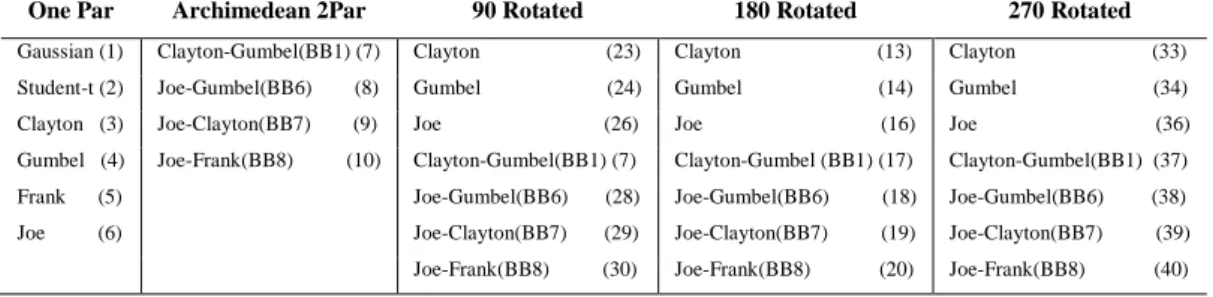
APPENDIX A: Dependence structure matrices ………..…….………….…...189
APPENDIX B: Plots of the fitted vine copula models……….…...…..…212
APPENDIX C: Portfolios’ efficient frontiers………..…….215
xii
LIST OF TABLES
Table 3-1: Gold and iron ore-nickel portfolios’ stocks’ names and codes ….…….… 40 Table 3-2: Coal-uranium and oil-gas portfolios’ stocks’ names and codes ……....….41 Table 3-3: Retail and manufacturing portfolios’ stocks’ names and codes ……….….42 Table 3-4: Mix-metals portfolio’s stocks’ name and codes ……..…….………..……42 Table 5-1: Set of the bivariate copula families employed by the vine copula models.70 Table 5-2: C-vine, d-vine and r-vine models’ bivariate copula selection for the gold
portfolio ………..………..…..…….…………72 Table 5-3: Significance testing of the gold portfolio’s relative comparison of
dependence……….………..…...………75 Table 5-4: C-vine, d-vine and r-vine models’ bivariate copula selection for the iron
ore-nickel portfolio ……….…………..……….………..….78 Table 5-5: Significance testing of the iron ore-nickel portfolio’s relative comparison of
dependence………...……….…..…80 Table 5-6: C-vine, d-vine and r-vine models’ bivariate copula selection for the
mix-metals leptokurtic portfolio ………..……..…. 84 Table 5-7: Significance testing of the mix-metals portfolio’s relative comparison of
dependence……….……..86 Table 6-1: C-vine, d-vine and r-vine models’ bivariate copula selection for the
coal-uranium portfolio ……….…....………...….92 Table 6-2: Significance testing of the coal-uranium portfolio’s relative comparison of
dependence………..………..…..….94 Table 6-3: C-vine, d-vine and r-vine models’ bivariate copula selection for the oil-gas
portfolio ………...………..…97 Table 6-4: Significance testing of the oil-gas portfolio’s relative comparison of
dependence………....……….……100 Table 7-1: C-vine, d-vine and r-vine models’ bivariate copula selection for the retail
portfolio ………...………..107 Table 7-2: Significance testing of the retail portfolio’s relative comparison of
dependence………..………...………...….110 Table 7-3: C-vine, d-vine and r-vine models’ bivariate copula selection for the
manufacturing portfolio ………...…………...……112 Table 7-4: Significance testing of the manufacturing portfolio’s relative comparison of
dependence……….115 Table 8-1: Optimal weights of the gold portfolio………....122 Table 8-2: Optimal weights of the iron ore-nickel portfolio ………..123 Table 8-3: Optimal weights of the mix-metals leptokurtic portfolio…………..……124 Table 8-4: Optimal weights of the coal-uranium portfolio………..………..….126
xiii
Table 8-5: Optimal weights of the oil-gas portfolio…………..……….…….…127 Table 8-6: Optimal weights of the retail portfolio………..……….128 Table 8-7: Optimal weights of the manufacturing portfolio……..……….………… 129 Table 8-8: Four-period scenario portfolios’ risk comparison for all risk measures ....131 Table 9-1: Significance testing of dependence concentration for the mining
portfolios……….138 Table 9-2: Significance testing of dependence concentration for the energy
portfolios……….140 Table 9-3: Significance testing of dependence concentration for the mining and energy
portfolios………...………..142 Table 9-4: Significance testing of dependence concentration for the mining and energy
portfolios and the retail and manufacturing portfolios……….……. 144 Table 9-5: Gold portfolio’s significance testing of dependence structure changes….146 Table 9-6: Iron ore-nickel portfolio’s significance testing of dependence structure
changes………...147 Table 9-7: Coal-uranium portfolio’s significance testing of dependence structure
changes………...148 Table 9-8: Oil-gas portfolio’s significance testing of dependence structure
changes………..………..….…..149 Table 9-9: Mix-metals portfolio’s significance testing of the dependence structure
changes……….………..150 Table 9-10: Retail portfolio’s significance testing of dependence structure changes.151 Table 9-11: Manufacturing portfolio’s significance testing of dependence structure
changes………..…………...152 Table 9-12: Goodness-of-fit testing for the gold, iron ore-nickel and coal-uranium
portfolios……….154 Table 9-13: Goodness-of-fit testing for the oil-gas, mix-metals and retail portfolios.155
Table 9-14: Goodness-of-fit testing for the manufacturing portfolio...156 Table 9-15: Goodness-of-fit testing summary……...………..…….…157
Table 9-16: Portfolios’ risk for the full sample, pre-GFC, GFC and post-GFC…..….159 Table 9-17: Full sample period portfolios’ risk rankings ………...…….160 Table 9-18: Degrees of freedom and critical values of observations………….……..162 Table 9-19: Significance t-testing of the portfolios’ optimal weights………..163 Table 9-20: Hypothesis testing results………..164
xiv
LIST OF FIGURES
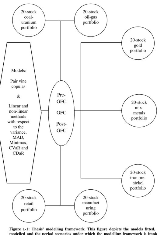
Figure 1-1: Thesis’ modelling framework………4
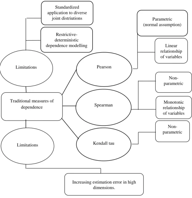
Figure 4-1: Modelling features and limitations of alternative measures of correlation...49
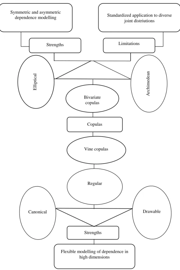
Figure 4-2: The bivariate copula and pair vine copula sets……….………..…50
Figure 4-3: Simplified 3-dimensional pair c-vine copula………..………51
Figure 4-4: An r-vine on 5 variables…….………...……….55
Figure 4-5: First two trees of an r-vine on 7 variables……...……….……..56
Figure 4-6: Diagonal matrix of an r-vine on 7 variables………...…….………...56
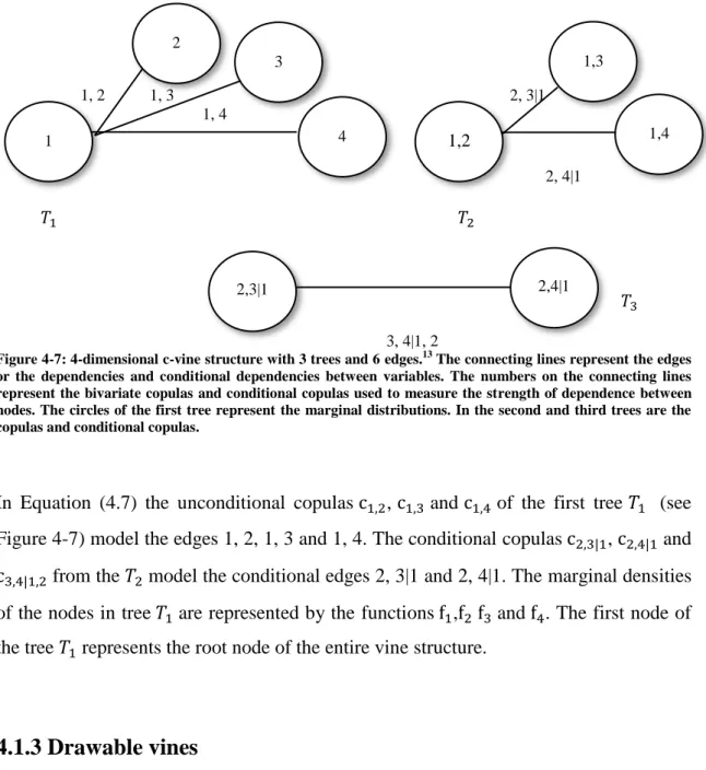
Figure 4-7: 4-dimensional c-vine structure with 3 trees and 6 edges……….…...58
Figure 4-8: 5-dimensional d-vine structure with 4 trees and 10 edges………….…….60
Figure 5-1: Dependence structure and Kendall tau matrices of the gold portfolio. ….71 Figure 5-2: Gold portfolio’s symmetric dependence concentration in the tails. …...76
Figure 5-3: Dependence structure and Kendall tau matrices of the iron ore-nickel portfolio……….77
Figure 5-4: Iron ore-nickel portfolio’s symmetric dependence concentration in the tails……….……81
Figure 5-5: Dependence structure and Kendall tau matrices of the mix-metals leptokurtic portfolio……….83
Figure 5-6: Mix-metals leptokurtic portfolio’s symmetric dependence concentration in the tails……….………..87
Figure 6-1: Dependence structure and Kendall tau matrices of the coal-uranium portfolio………....91
Figure 6-2: Coal-uranium portfolio’s symmetric dependence concentration in the tails………...95
Figure 6-3: Dependence structure and Kendall tau matrices of the oil-gas portfolio………96
Figure 6-4: Oil-gas portfolio’s relative comparison of symmetric dependence concentration in the tails……….…..99
Figure 7-1: Dependence structure and Kendall tau matrices of the retail portfolio….106 Figure 7-2: Dependence structure and Kendall tau matrices of the manufacturing portfolio………..………..111
Figure 8-1: Full sample period portfolios’ efficient frontiers for the CVaR measure……….…130
1
CHAPTER 1
INTRODUCTION
This chapter consists of seven sections: introduction and background, significance of the study, purpose, research questions, assumptions, definition of terms and thesis
outline.
The introduction and background section positions the research in the landscape of the
mining, energy, retail and manufacturing sectors and in the context of the 2008-2009 global financial crisis. The size of the sectors modelled and their significance to the Australia economy is acknowledged. The problem of accurately estimating the multivariate dependence of financial variables is stated and the modelling limitations of alternative measures for dependence and correlation estimation are pointed out. The emergence of new techniques for dependence estimation and portfolio optimization is pointed out and the relevance of the multiple risk measure-based portfolio optimization approach is recognized. Reasons for selecting the 2008-2009 GFC as the context to implement the modelling framework are given, along with motivations for the selection of the mining, energy, retail and manufacturing stock portfolios. The contributions of the research conducted are also stated in this section. The significance of the study
discusses the usefulness of the research undertaken, while the purpose and research
questions sections outline the research objectives and research questions. The
assumptions section states the assumptions upon which the research and modelling
framework implemented rest. Some key concepts and ideas are explained in the
2
1.1
Introduction and background
The Australian economy has grown along with the expansion of the mining and energy sectors, and in relation to the economic linkages these sectors have with the retail and manufacturing sectors (Bishop et al., 2013; KPMG Economics Group, 2013; McKay et al., 2000; Ahammad & Clements, 1999). As of December 2012 the percentages of mining (coal and uranium are included in this category) and energy (e.g. oil, gas and renewables) stocks listed and trading on the Australian Securities Exchange were approximately 39 and 9 respectively, an indication of the size of the resources sector and their relationship of dependence with the economy (Arreola & Powell, 2013). In the last two decades Australia saw a sharp increase in the mining of precious and non-precious metals such as gold, iron ore and nickel stemming from the Asian emerging economies’ increasing demand of those commodities (Bishop et al., 2013; Bingham & Perkins, 2012; Connolly & Orsmond, 2011; Gardner-Bond et al., 2008). Along with this trend of increasing demand, portfolio investors have more frequently been considering positions in the mining and energy sectors to diversify their holdings (Jennings, 2012). In 2011, gold, iron ore and nickel production placed Australia as the third, first and fourth largest exporter worldwide, respectively (Bingham & Perkins, 2012; Gardner-Bond et al., 2008). By 2014 energy production in Australia had placed the country as the ninth largest producer worldwide, with coal, uranium and natural gas accounting for 60, 20 and 13 per cent of the energy mix (BREE, 2014; DI et al., 2014).1
The retail and manufacturing sectors are important sectors of the Australian economy, not only because they account for 12 percent of total GDP but also because the retail sector appears to be on the rise, while the manufacturing sector has been in a declining trend and exhibits an increasing risk (Department of Industry, 2014; Kryger, 2014; Australian Bureau of Statistics, 2015). The retail sector’s good performance is most likely due to the economic linkages it has with the Australian resources sector, manufacturing sector and other sectors of the economy (ARA, 2014; Savills Research, 2014; Delloite, 2013; KordaMentha, 2013;CT, 2012; Green & Roos, 2012; NAB, 2012; Mehmedovic et al., 2011; DIISR, 2010). The levels of demand, spending and
1 The acronyms BREE, DI, GA, ARA,CT, NAB and DIISR used in the present chapterstand for Bureau of
Resources and Energy Economics, Department of Industry, Geoscience Australia, Australian Retailers Association, Commonwealth Treasury, National Australian Bank and Department of Innovation, Industry, Science and Research.
3
investment in the retail sector appear to be correlated with the performance of the Australian resources sector (KPMG Economics Group, 2103).
In this context of dependence relationships and economic linkages between the Australian resources sector and Australian economy and between the Australian resources sector and Australian retail and manufacturing sectors, the accurate estimation of dependence between financial variables and their optimization is a non-trivial task that requires the use of sophisticated techniques for dependence estimation and portfolio optimization. The most promising modelling techniques to address these issues have emerged in the form of pair vine copulas and risk measures threaded with linear and nonlinear optimization methods (see e.g. Arreola & Powell, 2013; Ghalanos, 2013; Czado et al., 2012; Czado, 2010; Dissmann, 2010; Aas et al., 2009; Heinen &Valdesogo, 2009; Bedford & Cooke, 2001,2002; Cooke, 1997; Joe, 1997). In tune with that wave of financial and statistical modelling this thesis implements, in the context of the 2008-2009 GFC and pre-GFC, GFC, post-GFC and full sample period scenarios, pair regular vines (r-vines), pair canonical vines (c-vines) and pair drawable vines (d-vines), and linear and nonlinear optimization methods with respect to the variance, mean absolute deviation (MAD), minimizing regret (Minimax), conditional Value-at-Risk (CVaR) and conditional Drawdown-at-Risk risk measures to examine the dependence risk profile, investment risk and portfolio allocation features of seven 20-asset portfolios from the gold, iron ore, nickel, coal, uranium, oil, gas, retail and manufacturing sectors of the Australian stock market.
The specific objectives of the vine copula modelling of dependence undertaken are to identify the dependence risk profile of the portfolios in specific market conditions, examine the changes of the portfolios’ dependence structure between pairs of period scenarios and recognize the vine copula models that best account for the portfolios’ multivariate dependence. The study looks at the assets’ dependence risk in times of financial turbulence characterized by low confidence in the financial stock markets, and in tranquil periods where the financial stock markets behave smoothly. The portfolios’ dependence structure changes are interpreted according to standard economic theory and the price behaviour of the assets’ underlying commodities across period scenarios. The multiple risk measure based portfolio optimization seeks to identify the least investment risky and most investment risky portfolios, single out the portfolio with the best risk-return trade-off and recognize the stocks that are good candidates for investment.
4
Figure 1-1: Thesis’ modelling framework. This figure depicts the models fitted, the data sets modelled and the period scenarios under which the modelling framework is implemented. The pair vine copula models fitted examine the multivariate interaction and dependence risk dynamics of the assets, while the fit of the linear and nonlinear optimization methods and risk measures looks at the characteristics of the minimum risk optimal portfolios. The modelling framework is implemented under four period scenarios: pre-GFC, GFC, post-GFC and full sample.
The motivation for the selection of the pair vine copula models to account for the multivariate dependence is that they are adequate to thoroughly examine the portfolios’ dependence risk dynamics in specific market conditions. Besides, the vine copula models overcome the restrictive and deterministic features of alternative measures of dependence and correlation such as the elliptical and Archimedean bivariate copulas
Models: Pair vine copulas & Linear and non-linear methods with respect to the variance, MAD, Minimax, CVaR and CDaR Pre-GFC GFC Post-GFC Full samp le perio d 20-stock gold portfolio 20-stock iron ore-nickel portfolio 20-stock coal-uranium portfolio 20-stock oil-gas portfolio 20-stock retail portfolio 20-stock mix-metals portfolio 20-stock manufact uring portfolio
5
and the Pearson, Spearman and Kendall tau (Brechmann & Czado, 2013). The portfolio optimization methods and risk measures considered are suitable because they set the ground to search for the stocks in which most of the optimization methods and risk measures assign weights which do not largely deviate from a mean of weights (i.e. the search for average model convergence). Besides, they provide a wide array of optimal investment scenarios that could cater for the investors’ risk and return preferences and enable a risk comparison of the portfolios (Arreola & Powell, 2013; Eling & Tibiletti, 2010; Krokhmal et al., 2002; Cheng & Wolverton, 2001; Stone, 1973).
The motivations for the selection of the gold, iron ore-nickel, mix-metals, coal-uranium, oil-gas, retail and manufacturing portfolios are their differences in terms of structure, volatility, uses and their importance in asset investment. The retail and manufacturing benchmark portfolios are included in the mix of portfolios because of the economic linkages they have with the mining and energy sectors (KPMG Economics Group, 2103; McKay et al., 2000; Ahammad & Clements, 1999). The 2008-2009 GFC event and period scenarios revolving around it provide the market conditions to compare the volatility changes and their effect on the portfolios’ dependence risk across period scenarios. Besides, the assets’ price behaviour can more easily be understood when the stock markets in financial turbulence and in tranquil periods are contrasted.
This thesis fills a gap in the literature of multivariate dependence modelling with pair vine copulas and in the literature of multiple risk measure-based portfolio optimization by introducing a “copula counting technique” and an “average model convergence” perspectives. The copula counting technique is a simple procedure for the analysis and interpretation of the portfolios’ multivariate interaction. The technique could be seen as an extension of unsystematic earlier attempts to dissect, organize and interpret the dependence structure of financial variables (see Allen et al., 2013; Dissmann et al., 2013; Czado et al., 2012; Heinen & Valdesogo, 2009). The average model convergence is a simple approach to handle and address in a more effective and objective manner the estimated multiple optimal weight allocations, the optimal stock selection and investment confidence problems underlying any type of portfolio optimization and faced by investors when having to select stocks from a wide array of investment scenarios.
6
1.2
Significance of the study
This thesis’ research is significant because of the following reasons:
1) It provides a comprehensive analysis and in-depth information about the dependence structure and dependence risk dynamics of the portfolios modelled and their underlying sectors. The adequate use of this information may lead portfolio investors to reduce losses and maintain gains during crisis periods and when the financial stock markets behave smoothly (CME Group, 2011; Singh & Vyas, 2011; Heywood et al., 2003). Portfolio managers and financial market analysts, who follow the trends and performance of the Australian mining and energy sectors may also benefit from the obtained assets’ dependence risk information by developing dependence risk and investment risk-adjusted portfolio management algorithms and investment strategies (Al Janabi, 2013). The results could also appeal to government agents whose responsibility is the stability of the macro economy. 2) It proposes a simple “copula counting technique” that simplifies the analysis and
interpretation of the assets’ dependence structure and dependence risk dynamics. The systematic aspect of the technique enables the non-specialized audience to easily access the information contained in the assets’ dependence structure matrix. 3) It proposes a simple “average model convergence” perspective to address the
optimal stock selection and investment confidence problems in a more objective manner through model convergence and model consensus thus, enabling the identification of the stocks in the portfolios that could be good candidates for investment.
7
1.3
Purpose
The purpose of the research conducted is to broaden the understanding on dependence risk in the Australian mining and energy stock portfolios modelled and their underlying sectors. It is also of interest to identify, through the use of the copula counting technique proposed, the specific market conditions under which one sector stock portfolio is riskier than others. In doing so, new insights and useful information are provided that could be used to develop dependence risk and investment risk-adjusted strategies for investment, rebalancing and hedging that more adequately account for downside risk. The portfolio optimization component of this thesis aims at examining the investment risk and resource allocation features of the asset portfolios. Another objective of the research conducted is to make the investors’ stock selection process simpler and less uncertain by employing model convergence and model consensus.
1.4
Research questions
1. Are there mining portfolios with higher dependence risk than others? 2. Are there energy portfolios with higher dependence risk than others?
3. Are there mining portfolios with higher dependence risk than energy portfolios? 4. Are there mining and energy portfolios with higher dependence risk than retail and
manufacturing benchmark portfolios?
5. Are the portfolios’ dependence structure changes between period scenarios statistically significant?
6. Is there a pair vine copula model that best captures the multivariate dependence structure of the portfolios?
7. Is there a portfolio of stocks that offers the best risk-return trade-off?
8. Is the average model convergence of the stocks’ optimal weights statistically significant?
8
The first research question seeks to identify the dependence risk differences between the mining portfolios: gold, iron ore-nickel and mix-metals. The second research question aims at identifying the dependence risk differences between the energy portfolios: coal-uranium and oil-gas. The third research question intends to compare the dependence risk differences between the mining and energy portfolios. The fourth research question examines the dependence risk differences between the mining and energy portfolios and the retail and manufacturing benchmark portfolios. The fifth research question wonders if the portfolios’ dependence structure changes between pairs of period scenarios are statistically significant. The sixth research question recognizes the importance of identifying the pair vine copula models that best account for the multivariate dependence structure of the portfolios. The seventh research question targets the identification of the portfolio with the best risk-return trade-off. The last research question examines if the difference between the average of the optimal weights and each of the optimal weights is statistically significant.
1.5
Assumptions
1. The stock return series employed for the vine copula modelling of dependence risk and portfolio optimization reflect all the effects exerted by the price drivers of the mining, energy, retail and manufacturing stocks (Clarke et al., 2001; Jordan, 1983). 2. The mining, energy, retail and manufacturing stock portfolios are representatives of
the underlying sectors.
3. Portfolio investors care about the skewed and leptokurtic features of their portfolio investments.
4. No short selling is considered in the optimization of the portfolios.
The first assumption acknowledges that the price and return series used to implement the modelling framework proposed reflect the idiosyncratic (i.e. company related) and systematic (i.e. market related) effects of the stock market. The validity of the statistical analysis rests on this assumption and implies that the stock price and return series cannot capture the effects from all existing price drivers. The second assumption is a
9
necessary condition for the drawing of generalizations about the dependence risk profile and investment risk features of the portfolios. This assumption recognizes the difficulty to model at once all the existing stocks trading in the ASX. The third assumption, along with Xiong and Idzorek (2011), Patton (2004) and Chunhachinda et al. (1997) acknowledges the importance of considering the skewness and kurtosis of the return distribution when optimizing stock portfolios. The fourth assumption discards the selling of some stocks in the portfolios and the reinvestment of the proceeds in other stocks. The discarding of short selling in the optimization implies that negative weights are not allowed.
1.6
Definition of terms
Correlation:
There is three commonly used traditional measures of correlation: the Pearson, the Spearman and the Kendall tau. Despite their differences they all share the same restrictive and deterministic features for dependence estimation. Specifically, they are designed to be fitted in a standardized manner to diverse pairs of variables’ joint distributions (Brechmann & Schepsmeier, 2013). The Pearson correlation measure is parametric, implying that it is built under the assumption of normality in the observations. The Spearman and the Kendall tau are non-parametric measures thus; do no impose any distributional constraint on the observations (Tsay, 2005; Chen & Popovich, 2002).
Cumulative distribution function:
A cumulative distribution function is defined as the probability that a random variable 𝑋 takes a value which is less than or equal to 𝑥 or, 𝐹 (𝑥) = 𝑃 (𝑋 ≤ 𝑥). The behaviour of the random variable is determined by the probability distribution function employed in
10
the modelling (Tsay, 2005). In this thesis, the cumulative distribution is represented by the stocks’ return distribution.
Marginal distribution:
Let the random variables 𝑋 and 𝑌 have a joint probability distribution 𝑝 (𝑥, 𝑦). The distribution of 𝑋, or alternatively the distribution of 𝑌, is viewed as the marginal distribution if either of them is treated separately. For instance, a data sample is considered to have a marginal distribution if it has been drawn from a larger data sample characterized by a certain probability distribution (Kijima, 2002). Although, the marginal distribution of the subsample is related to the distribution of the original data sample, it is treated as if it has its own identity. In this thesis each stock from each of the portfolios modelled represents a marginal distribution.
Normal distribution:
It is a probability distribution function with most of the observations located around the mean. The standard normal distribution function has a zero mean and a variance equal to 1. The standard normal distribution’s variance keeps most of the observations around the mean and discourages extreme fluctuations. A random variable 𝑋 is standard normally distributed if it satisfies:
𝑓(𝑥) =𝑒
−(𝑥−𝜇)2 2𝜎2
√2𝜋𝜎 (1.1)
where 𝜇 and 𝜎2 are the mean and variance parameters (Kijima, 2002). The standard normal distribution is also known as the Gaussian distribution and equation (1.1) represents the standard normal density function, which enables to observe the bell shape distribution of a random variable that satisfies the mean and variance normal conditions.
11
Kendall tau:
The Kendall tau correlation measure is non-parametric and as such does not impose any constraint on the distribution of the observations. The Kendall tau equation of the variables X and Y is:
𝜌𝜏(𝑋, 𝑌) = 4 ∫ ∫ 𝐶(𝑢, 𝑣)𝑑𝐶(𝑢, 𝑣) − 101 01 (1.2) where 𝜌𝜏 represents the Kendall tau measure, 𝐶(𝑢, 𝑣) is the copula of the joint distribution and, 𝑑 is the differential applied to 𝐶(𝑢, 𝑣).
Skewness:
It is the third central moment of a random variable and can be interpreted as “the propensity to generate negative returns with greater probability than suggested by a symmetric distribution” (Albuquerque, 2012). In this thesis the negative skewness is of concern because its effects are reflected in the left tail of the return distribution, the domain of the loss function (Kim et al., 2014; Prakash et al., 2003; Barone-Adesi, 1985; Kane, 1982; Chunhachinda et al., 1997; Lai, 1991).
𝑆 = √𝑛∑ (𝑥𝑖− 𝜇𝑥)3 𝑁 𝑖=1 (∑𝑁 (𝑥𝑖 − 𝜇𝑥)2 𝑖=1 ) 3 2 ⁄ Kurtosis:
The kurtosis is the fourth central moment of a random variable and accounts for the observations falling in the tails of the distribution. This statistical and distributional characteristic is of interest in this thesis because the stocks’ asymmetric and symmetric dependence takes place in the tails of the variables’ distribution (Tsay, 2005). An equation of the kurtosis is:
12 𝐾(𝑥) = 𝑛 ∑ (𝑥𝑖−𝜇𝑥) 4 𝑁 𝑖=1 (∑𝑁𝑖=1(𝑥𝑖−𝜇𝑥)2)2 (1.3) Asymmetric dependence:
The concept of asymmetric dependence refers to the greater correlation stock return series tend to have in the tails (Hatherley, 2009; Tsafack, 2009; Alcock & Hatherley, 2008). In a macroeconomic setting, financial stock markets have been observed to display greater correlation in the negative tail when the financial stock markets lack confidence (Aloui et al., 2011; Patton, 2004; Ang & Chen, 2002; Erb et al., 1994).
The theorem of Sklar:
The theorem of Sklar (1959) shows that the multivariate distribution of a data set can be decomposed into copulas and marginal distributions. The theorem plays an important role in the statistical framework upon which the pair vine copula models are built (Brechmann & Schepsmeier, 2013). Analytically, let the random variables 𝑋1, … , 𝑋𝑛 have a continuous distribution function 𝐹1, … , 𝐹𝑛 and corresponding joint distribution
function 𝐹(𝑥1, … , 𝑥𝑛). It follows that a copula C exists such that,
𝐹(𝑥1, … , 𝑥𝑛) = C(𝐹1(𝑥1), … 𝐹𝑛(𝑥𝑛)) (1.4) for all 𝒙 = (𝑥1, … , 𝑥𝑛)′∈ ℝ𝑛. Applying a probability integral transform on Equation (1.4) yields:
𝐹(𝐹1−1(𝑥
1), … , 𝐹𝑛−1(𝑥𝑛)) = C(𝑢1 , … , 𝑢𝑛) (1.5)
13
Copula counting technique:
The copula counting technique is proposed in this thesis to dissect, organize, analyse and interpret the dependence structure of the portfolios modelled. It enables an in-depth and comprehensive analysis of the assets’ symmetric and asymmetric dependence risk features in specific market conditions. The technique consists of five stages: counting, recording, classification, grouping and aggregate dependence reading.
Dependence risk:
The concept of dependence risk refers to the risk stemming from the specific type of dependence relationship two variables have during times of financial turbulence and when the financial stock markets behave smoothly. The interaction between two variables during times of financial turbulence tends to be more uncertain and less predictable because of the liquidity shrinkage in the financial system. As a consequence, the dependence risk two variables have in the negative tail is higher in those market conditions. Campbell et al. (2002) find that stock securities tend to correlate more
strongly when the financial stock markets are unstable. The dependence risk two stock
return series have in the centre of the joint distribution is featured by mild swings in the return distribution. The dependence risk two stock return series have in the tails is characterized by large swings in the return distribution. The dependence risk of two variables could be linear, nonlinear, symmetric and asymmetric. It should also be noted that a relationship exists between dependence risk and the tail dependence coefficient, with changes in the tail dependence coefficient determining the characteristics of the dependence risk. The relationship between the tail dependence coefficient and dependence risk is reflected as stronger or weaker correlation caused by large positive or negative return variations.
14
Dependence concentration:
Is based on and presupposes the aggregation of bivariate copulas selected by the vine copulas to model and estimate the dependence structure of the portfolios. It refers to the location in the joint distributions where pairs of variables experience higher correlation activity, as indicated by the specific type of bivariate copulas aggregated.
Average model convergence:
The average model convergence is proposed to handle the multiple optimal weight allocations, resulting from the fit of the various portfolio optimization model specifications, and address the optimal stock selection and investment confidence problems underlying any type of portfolio optimization. The approach identifies as good candidates for investment the stocks to which most of the optimization methods and risk measures assign weights that do not largely deviate from a mean of the optimal weights.
1.7
Thesis outline
This chapter positions the research conducted in this thesis in the context of the Australian mining, energy, retail and manufacturing sectors. Motivations for the selection of the data sets and modelling framework implemented are given and this thesis’ contributions and their significance are stated. Chapter 2 reviews the relevant literature in the fields of bivariate copulas, pair vine copulas and multiple risk measure-based portfolio optimization. The pair vine copula, portfolio optimization and hypothesis testing methodologies are explained in Chapter 3. Chapter 4 lays the mathematics and statistics of the pair vine copula and portfolio optimization model specifications considered. In Chapter 5 the copula counting technique is applied to examine the dependence structure of the mining portfolios. In Chapter 6 the copula counting technique is implemented to examine the dependence structure of the energy portfolios. In Chapter 7 the copula counting technique is employed to understand the dependence structure of the retail and manufacturing benchmark portfolios. In Chapter 8 linear and nonlinear optimization methods with respect to five risk measures are fitted
15
to estimate the minimum risk optimal portfolios, identify the stocks that could be good candidates for investment and establish a risk comparison between portfolios. Chapter 9 deals with the testing of hypothesis and Chapter 10 discusses the main research findings, topics for further research and conclusions.
1.8
Summary
This chapter introduced the research conducted in this thesis and positioned it in the context of the mining, energy, retail and manufacturing sectors, and the 2008-2009 global financial crisis. The modelling framework implemented was explained and motivations for the selection of the data sets were given. The objectives and purpose of the research conducted were stated and its contributions and significance were pointed out. This thesis’ modelling framework was indicated to consist of pair vine copulas, risk measures and optimization methods. The main contributions of the research are indicated to stem from the use of the copula counting technique and average model convergence perspectives. The research undertaken was recognized to be significant to portfolio managers, portfolio risk managers, investors and government agents whose responsibility is the stability of the macro economy.
16
CHAPTER 2
REVIEW OF THE LITERATURE
This chapter consists of four sections: graphical models, bivariate copula models, pair vine copula models, and risk measures and portfolio optimization models. The literature
is surveyed chronologically, with the most recent literature discussed last.
The graphical models section highlights some of the key ideas and concepts underlying
the path of coefficients method of Wright (1934) and their connection to the pair vine copula models fitted in this thesis. Two central concepts in this section are flexibility and branching sequential ordering. The bivariate copula models section looks at studies dealing with the modelling of dependence of financial variables using bivariate copulas. The central role of the bivariate copulas for the development of the pair vine copulas is recognized and the comparative advantage of the bivariate copulas relative to the traditional measures of correlation is acknowledged. The pair vine copula models
section concentrates on the literature dealing with pair vine copula developments and applications. Studies comparing the fit of the r-vines, c-vines and d-vines are also reviewed. Key concepts in this section are pair copula constructions, multivariate density decomposition and inference of pair vine copula structures. The gap filled in the literature of dependence modelling with pair vine copulas is discussed in this section too. The risk measures and portfolio optimization models sectionsreview the portfolio optimization literature dealing with applications of the variance, conditional Value-at-Risk (CVaR), conditional Drawdown-at-Risk (CDaR), minimizing regret (Minimax) and mean absolute deviation (MAD) risk measures. The gap filled by the average model convergence in the literature of multiple risk measure-based portfolio optimization is also indicated in this section.
17
2.1 Graphical models
Graphical models such as pair vine copulas are considered in this thesis because of their suitability to visualise and represent a problem in a simple, flexible and dissectible manner (Lauritzen, 1996). Graphical structures, in addition to that, appear to be naturally adequate to represent the interaction variables through nodes-vertices and edges thus, facilitating the estimation of dependence and the inference of causality (Guo et al., 2010).
The use of graphical models to account for the interaction between variables goes back to Wright’s (1934) work where graphical path analysis, by means of the path of coefficients method, is pursued to link parent-child heritable relationship of species. The path of coefficients method is acknowledged for its flexibility to associate within a system the correlation coefficients. This flexibility aspect of Wright’s path of coefficients method appeals to the pair vine copula modelling of dependence because the main strength of the pair vine copula models stems from their flexibility (Brechmann & Schepsmeier, 2013). 2 Both modelling frameworks however differ in their ability to account for nonlinearities in the joint distributions. The pair vine copulas are specifically designed to capture the nonlinear relationship between variables (Heinen & Valdesogo, 2009).
Another point of connection between Wright’s path of coefficients method and the pair vine copula models relates to the branching sequential ordering of the variables. Both modelling techniques branch the variables to facilitate the estimation of dependence (see Czado et al., 2012; Dissmann, 2010). The path of coefficients method, in addition to that, estimates the correlation between two variables according to the shape of their joint distribution and the specific type of relationship each of the variable has with other variables within the system. This model feature of conditioning the correlation estimates on the type of relationship each of the variables has with other variables resembles the pair vine copula estimation of dependence. Specifically, conditional densities are used to account for the conditional dependencies (Brechmann & Schepsmeier, 2013; Czado, 2010).
2 There is a tightly interwoven relationship between flexibility and structure in the graphical vine copula
models. It is in fact the combination of flexibility and structure what leads to greater accuracy in the modelling.
18
Blalock (1971), Neopolitan (1990) and Cox and Wermuth (1996) have also developed and applied graph theory to model the dependence relationship between variables. The latter, in the context of large systems, uses graphs to represent the dependence and independence of variables. Neopolitan (1990) implements Bayesian networks involving paths, cycles, cliques, triangulation and belief networks to account for the relationships between variables. Blalock (1971) models the causality of variables using graphical structures.
2.2 Bivariate copula models
The copula approach in the form of bivariate copulas has been proposed for overcoming the limitations of alternative measures of correlation such as the Pearson, Spearman and Kendall tau. The elliptical and Archimedean bivariate copulas are known for providing good estimates of the underlying interaction of financial variables and for being the building blocks of the pair vine copula models (Brechmann & Czado, 2013; Low et al., 2013).
The first study to implement a copula-like modelling approach without employing the term “copula” is said to be Hull and White (1998). Their study maps the distribution of twelve currency exchange rates taking into account the changes in the market’s factors driving the currency co-movements. The market factor’s co-movements are estimated using suitable joint probability distribution functions. Hull and White’s freedom to select adequate joint probability distribution functions in the modelling of dependence is a feature found in the pair vine copula modelling of dependence. Specifically, joint probability distribution functions such as bivariate copulas can be manually selected to build a vine structure that represents a statistical model (see Brechmann & Schepsmeier, 2013; Dissmann, 2010). Hull and White’s approach to dependence estimation, just as any type of bivariate copula modelling, lacks the flexibility to accurately model high dimensional multivariate dependence structures. The bivariate copulas however, relative to the joint probability distribution functions employed by Hull and White, have the comparative advantage of splitting the joint distributions into copulas and marginals, while preserving the marginals’ original distribution (Patton, 2012a).
19
Embrechts et al. (1999) are acknowledged in the literature of bivariate copulas for being the first to associate the concept of “copula” with measures of dependence in finance. Their study compares the fit and performance of the Student-t bivariate copula with the fit of the Pearson correlation measure. As expected, they found the Pearson correlation estimates to represent poorly the interaction between variables. The Student-t copula, on the other hand, better captures the distribution in the tails, while providing more information about the interaction between variables. Embrechts et al.’s research has in common with this thesis’ research the recognition of the bivariate copulas as more accurate and adequate than the traditional measures of correlation (Brechmann et al., 2014; Brechmann & Czado, 2013).
Li (2000) employs bivariate copulas to model the correlation structure of credit risk portfolios. The study equates the survival times of credit risks (a credit risk is a fund borrowing company) with the marginals and uses the marginals to build correlation structures. The bivariate copulas are also employed to measure the credit risks’ default correlation. Li’s modelling framework has in common with the pair vine copula models the notion and use of correlation structures. The correlation structure concept alludes to the concept of dependence structure that is central in the pair vine copula literature. One topic often appearing in early applications of bivariate copulas to model the interaction between financial variables is about the comparison of the Gaussian bivariate copula with the Student-t bivariate copula (e.g. Tong et al., 2013; Berg & Aas, 2009; Fischer et al., 2009; Junker & May, 2005; Malevergne & Sornetten, 2003; Embrechts et al., 1999). Despite its limitations, the Gaussian copula became a dominant model for dependence estimation due to its simplicity of application and tractability. The emergence of the Student-t copula and its symmetric dependence modelling of the tails led to the comparison of both copulas in terms of fit and performance (see e.g. Arreola et al., 2013; Malevergne & Sornetten, 2003).
Malevergne and Sornetten (2003) is one of those studies comparing the Gaussian and Student-t bivariate copulas in the context of a financial crisis event. They do so by modelling the interaction between exchange rates from six countries, six metals traded on the London Metal Exchange, and 22 large cap stocks from the New York Stock Exchange. They find the Gaussian copula to produce good estimates for normally distributed data sets in non-crisis periods, while the Student-t copula adequately captures the distribution in the tails for non-crisis periods. A point of connection between Malevergne and Sornetten’s (2003) research and this thesis’ research lies in the
20
use of financial period scenarios as the context to implement their modelling framework. Both studies specifically, appear to understand the importance of considering financial crisis events to better understand the dependence risk behaviour of financial variables in stress-testing and tranquil time periods.
Junker and May (2005) establish a comparison between bivariate copulas by fitting them to a stock portfolio consisting of six assets from the German and USA markets. Their modelling framework considers the transformed Frank copula, Gaussian, Student-t, and a Clayton copula based on a linear convex combination. They model the marginals by employing the Pareto distribution that is often used in Extreme Value Theory to account for the leptokurtic features in the tails of the marginals (Këllezi & Gilli, 2000). Their findings indicate that the transformed Frank copula produces the best results. The combination of the Frank copula with the Pareto distribution captures the dependence in the tails best. Junker and May’s research and this thesis’ research share the concern about accounting for the asymmetric dependence in the tails during crisis periods.
An important topic in the literature of bivariate copula modelling is that of contagion across financial stock markets (e.g. Barunik & Vacha, 2013; Ozkan & Unsal, 2012; Kazi et al., 2011; Kenourgios et al., 2010; Markwat et al., 2009a; Chiang et al., 2007;
Bae et al., 2003). Contagion refers to the transmission of economic conditions from one
financial stock market to another (Corsetti et al., 2001). The subject of contagion has gained increasing attention since the 2008-2009 GFC took place and due to the expanding global economy (Poirson & Schmittmann, 2013).
Two pieces of research that have examined the contagion phenomenon across international stock markets are Chen and Poon (2007) and Rodriguez (2007). The former fits time-varying Student-t bivariate copulas and a dummy Student-t copula to examine the contagion effects between 28 of the largest capitalized financial stock markets (including Argentina, Chile, The Philippines and Russia) in the context of the Asian crisis of 1997. They find the European countries to have the strongest contagion effects. Their research connects to this thesis’ research in the consideration of a financial crisis event as the context to implement their modelling framework. Rodriguez’s (2007) piece of research, relative to that by Chen and Poon (2007), models two financial crisis events: the Asian crisis of 1997 and the Mexican crisis of 1994.
21
Rodriguez’s (2007) approach to dependence modelling is based on “switching copula” versions of the Frank, Gumbel, Clayton and the Student-t with time-varying parameters. These copulas are indicated to capture adequately the symmetric and asymmetric dependence, and the increases and decreases of tail dependence. Rodriguez models the marginal distributions by fitting a SWARCH method that lets the variance of the variables to shift occasionally according to a Markov process. His findings indicate the presence of increased tail and asymmetric dependence in the Asian countries during the crisis period. The pair Mexico-Brazil displays symmetric dependence, while the pairs Thailand-Indonesia and Thailand-Korea display greater dependence in the centre of the joint distribution during tranquil periods. Rodriguez’s research and this thesis’ research have in common the consideration of crisis events as the context to implement their modelling framework. His modelling approach has the comparative advantage of using copulas with time varying parameters (Ausin & Lopes, 2010).
In the bivariate copula literature, applications assuming the parameters of the bivariate copulas to remain constant over time are seen as less complicated in terms of implementation, and less sophisticated in terms of the accuracy they provide; relative to letting the bivariate copula parameters change in time (Hautsch et al., 2013;Markwat et
al., 2009b). Tong et al. (2013) and Wen et al. (2012) along with Chen and Poon (2007)
and Rodriguez (2007) relax that assumption by letting the parameters of the bivariate copulas change over time thus, obtaining more accurate estimates of the multivariate dependence from energy markets.
Tong et al. (2013) model the positive and negative asymmetric tail dependence between
crude oil and refined petroleum markets by fitting thirteen different copulas with time varying parameters. Among the copulas they consider are the Gaussian, Student-t, Clayton, Gumbel, Symmetrized Joe-Clayton, mixed Clayton, mixed Gumbel, asymmetric logistic model and mixed asymmetric logistic model. The mixed asymmetric logistic copula is identified to best fit the data sets, while the crude oil and refined petroleum markets are found to move in similar directions. Wen et al. (2012) specifically examine the interaction between the WTI (West Texas Intermediate),
S&P500 and the Shanghai and Shenzhen composite indices.3 Their results indicate the presence of tail and symmetric dependence between the energy, US and Chinese indices
3
WTI is used for the modelling of energy market most likely because it is used in the Chicago Mercantile Exchange as the commodity that underlies oil futures contracts and as such it is often employed as a benchmark in the modelling of global energy markets (Vassiliou, 2009).
22
during the crisis period. The contagion effects between the WTI and Chinese indices are acknowledged to be weaker as compared to those between the WTI and S&P500. Their research connects to this thesis’ research in the modelling of dependence in energy markets and the consideration of a financial crisis event. Unlike their research this thesis’ research does not use copulas with time varying parameters because the copula models used suffice to account for the dependence concentrated at various locations of the joint distributions.
Patton (2012a, 2012b) discusses model selection, parameter estimation through maximum likelihood, model fit, and parametric and semi-parametric inference methods for model estimation. Aloui et al. (2013) estimate the conditional dependence between the Brent Crude Oil and the Central and Eastern European economies.
2.3 Pair vine copula models
In the literature of pair vine copulas Joe (1997) is seen as the starter of a series of developments. He discusses multivariate copula constructions for the design of various types of dependence structures and introduces maximum likelihood methods for the estimation of bivariate copula parameters. His research is of specific relevance to this thesis’ research in that it lays some of the theoretical and statistical ground on which some of the modelling implemented in this thesis is based. Bedford and Cooke (2002, 2001) develop an equation for the construction and inference of multivariate pair copulas. Cooke (1997) employs flexible graphical vine trees or “trees of dependent random variables” to organize joint probability distributions of multiple characteristics. Berg and Aas (2009) focus on the comparison of pair vine copula constructions with nested Archimedean constructions. In their modelling of a precipitation data set and a financial data set consisting of the British Petroleum, Exxon Mobile, Deutsche Telekom and France Telecom stocks they find the pair vine copula constructions to be more flexible than the Archimedean constructions. They find the fitted Student-t pair vine copula construction to best fit the financial data set, while the Gumbel pair vine copula construction bests accounts for the dependence of th