Chapter 2
Mathematical Model of the Safety Factor
and Control Problem Formulation
We are interested in controlling the safety factor profile in a tokamak plasma. As the safety factor depends on the ratio of the normalized radius to the poloidal magnetic flux gradient, controlling the gradient of the magnetic flux allows controlling the safety factor profile. In this chapter we present the reference dynamical model [1] for the poloidal magnetic flux profile and its gradient (equivalent to the effective poloidal field magnitude, as defined in [2]), used throughout the following chapters, as well as the control problem formulation. Some of the main difficulties encountered when dealing with this problem are also highlighted.
2.1 Inhomogeneous Transport of the Poloidal Magnetic Flux
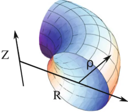
The poloidal magnetic flux, denotedψ(R,Z), is defined as the flux per radian of the magnetic field B(R,Z)through a disc centered on the toroidal axis at height Z, having a radius R, see Fig.2.1. A simplified one-dimensional model for this poloidal mag-netic flux profile is considered. Its dynamics is given by the following equation [3]:∂ψ ∂t = ηC2 μ0C3 ∂2ψ ∂ρ2 + ηρ μ0C32 ∂ ∂ρ C2C3 ρ ∂ψ ∂ρ + η∂∂ρV Bφ0 FC3 jni (2.1)
with the geometry defined by:
ρ .= φ πBφ0, C2(ρ) .= ∂V ∂ρ ρ2 R2 , C3(ρ) .= ∂V ∂ρ 1 R2
where·represents the average over a flux surface, indexed by the equivalent radius ρ. The remaining coefficients are: φ, the toroidal magnetic flux; Bφ0, the value of the toroidal magnetic flux at the plasma center; η, the parallel resistivity of the plasma; andμ0, the permeability of free space. jniis a source term representing the
F. Bribiesca Argomedo et al., Safety Factor Profile Control in a Tokamak, 11 SpringerBriefs in Control, Automation and Robotics,
Fig. 2.1 Coordinate system (R,Z)used in this chapter
total effective current produced by non-inductive current sources. F is the diamag-netic function and ∂∂ρV is the spatial derivative of the plasma volume enclosed by the magnetic surface indexed byρ. A summary of these variables can be found in Appendix B.
With the following simplifying assumptions:
• ρ <<R0(usually referred to as the cylindrical approximation, where R0is the
major radius of the plasma);
• the diamagnetic effect caused by poloidal currents can be neglected, the coefficients
C2, C3and F simplify to:
F ≈R0Bφ0, C2(ρ)=C3(ρ)=4π2 ρ
R0
and the spatial derivative of the enclosed plasma volume becomes: ∂V
∂ρ =4π
2ρ R0
Introducing the normalized variable r=. ρ/a, a being the minor radius of the last
closed magnetic surface, we obtain the simplified model [1,4]: ∂ψ ∂t (r,t)= η(r,t) μ0a2 ∂2ψ ∂r2 + 1 r ∂ψ ∂r +η(r,t)R0jni(r,t) (2.2)
with the boundary condition at the plasma center: ∂ψ
∂r(0,t) = 0 (2.3)
2.1 Inhomogeneous Transport of the Poloidal Magnetic Flux 13 ∂ψ ∂r(1,t)= − R0μ0Ip(t) 2π or ∂ψ ∂t (1,t)=Vloop(t) (2.4)
(where Ipis the total plasma current and Vloopis the toroidal loop voltage) and with
the initial condition:
ψ(r,t0)=ψ0(r)
Remark 2.1 The validity of this model (derived for Tore Supra) can be extended to
other tokamaks by changing the definition of the values C2, C3, F and∂∂ρV.
2.2 Periferal Components Influencing the Poloidal
Magnetic Flux
The dynamics (2.2) depend on the plasma resistivity (diffusion coefficient), the induc-tive current generated by the poloidal coils (boundary control input) and the non-inductive currents (distributed control input and nonlinearity), which can be described as follows.
2.2.1 Resistivity and Temperature Influence
The diffusion term in the magnetic flux dynamics is provided by the plasma resistivity η, which introduces a coupling with the temperature (main influence) and density profiles. This parameter is obtained from the neoclassical conductivity proposed in [5] (approximate analytic approach) using the electron thermal velocity and Braginskii time, computed from the temperature and density profiles as in [6].
The temperature dynamics are typically determined by a resistive-diffusion equation [2], where the diffusion coefficient depends nonlinearly on the safety factor profile [7]. A quasi-1D model was proposed in [8] to model the normalized tem-perature profiles as scaling laws determined by the global (0-D) plasma parameters and to constrain the temperature dynamics by the global energy conservation. This grey-box model was shown to provide a sufficient accuracy for the magnetic flux prediction in [1].
The resistive-diffusion time is much faster (more than 10 times) than the current density diffusion time, which motivated lumped control approaches based on the separation of the timescales and using a linear time-invariant model [9, 10]. In our case, we consider thatηvaries in time and space, to avoid the strong dependency on the operating point, but we do not address specifically the problem of a coupling with the temperature dynamics (thus considering only the linear time-varying contribution of the resistivity).
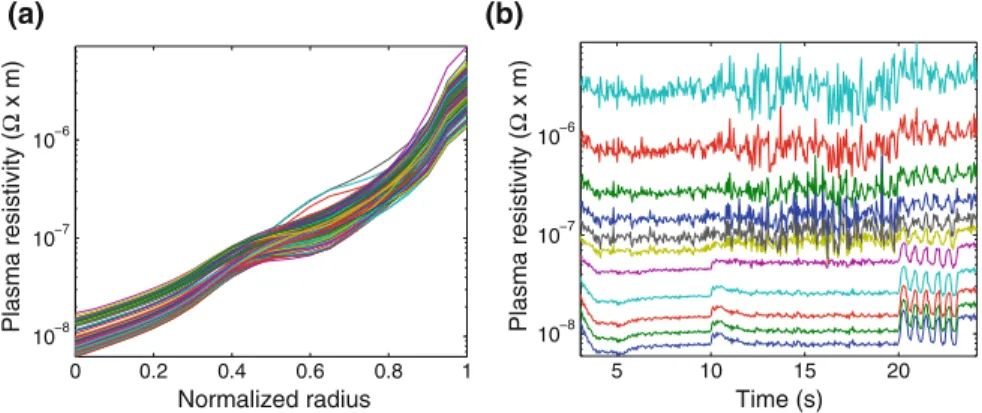
As an example, the resistivity calculated with measured temperature profiles is depicted in Fig.2.2. This plasma shot is characterized by power modulations of the
0 0.2 0.4 0.6 0.8 1 10−8 10−7 10−6 Plasma resistivity ( Ω x m) Normalized radius 5 10 15 20 10−8 10−7 10−6 Plasma resistivity ( Ω x m) Time (s) (a) (b)
Fig. 2.2 a Spatial distribution for different time instants. b Time evolution at different locations. Plasma resistivity profiles computed for Tore Supra shot 35952 (modulations on the LH and ICRH antennas)
lower hybrid (LH) and ion cyclotron radio heating (ICRH) antennas. Note the differ-ence of three orders of magnitude between the plasma center and its edge on Fig.2.2a, and the modulated and noisy time-evolution on Fig.2.2b. The crewels observed after 20 s result from LH modulations (step inputs) at relatively low power and illustrate an input-to-state coupling effect, as LH is our main input on the magnetic flux.
2.2.2 Inductive Current Sources
The magnetic flux at the boundary ∂∂tψ(1,t)is set by the poloidal coils surrounding the plasma and the central solenoid, and constitutes the inductive current input. This can be described by the classical transformer model where the coils generate the primary circuit while the plasma is the secondary, modelled as a single filament. The dynamics of the coils current Ic(t)and of the plasma current Ip(t)are coupled as [11]:
Lc M M Lp d dt Ic Ip = − Rc 0 0 Rp Ic Ip + Vc RpINI
where Rcand Lcare the coils resistance and internal inductance, Rpand Lpare the
plasma resistance and inductance, M is the matrix of mutual inductances, Vcis the
input voltage applied to the coils and INIis the current generated by the non-inductive
sources. Note that the values of Rcand Lcare given from the coil properties while
M is obtained from an equilibrium code (i.e. CEDRES++[12]). Considering the effects of the plasma current and inductance variations, the loop voltage Vloop is
2.2 Periferal Components Influencing the Poloidal Magnetic Flux 15 Vloop(t)= − 1 Ip d dt LpIp2 2 +MdIc dt
In practice, a local control law is set on the poloidal coils to adjust the value of Vc
according to a desired value of Vloop, which can be measured with a Rogowski coil.
If the reference is set on the plasma current Ipinstead, then Vcis such that the coils
provide the current necessary for completing the non inductive sources to obtain Ip.
2.2.3 Non-inductive Current: Sources and Nonlinearity
The non-inductive current jni in the magnetic flux dynamics (2.2) is composed of
two types of sources: the controlled inputs and the bootstrap effect.
The controlled inputs are the current drive (CD) effects associated with neutral beam injection (NBI), traveling waves in the lower hybrid (LH) frequency range (0.8–8 GHz, the most effective scheme) and electron cyclotron (EC) waves. The precise physical modeling of the CD effects necessitates a complex analysis of the coupling between waves and particles, which cannot be used for real-time control purposes. We consider instead some semi-empirical models for the Lower Hybrid Current Drive (LHCD) and Electron Cyclotron Current Drive (ECCD) antennas (NBI is not explicitly included in our control schemes but the general strategy would remain the same), where the current deposit shape is constrained to fit a gaussian bell [1]. The gaussian shape is identified from experimental data (LHCD) or obtained from model simplifications (ECCD), while the amplitude of the deposit comes from CD efficiency computations involving the density, temperature and total current of the plasma.
For example the shape of LHCD deposit can be adequately approximated by a gaussian curve with parameters μ,σ and Alh (which depend on the engineering
parameters Plhand N||and on the operating point) as:
jlh(r,t)=Alh(t)e−(r−μ(t)) 2/(2σ2(t))
,∀(r,t)∈ [0,1] × [0,T] (2.5) Scaling laws for the shape parameters can be built based on suprathermal electron emission, measured via hard X-ray measurements, see for instance [14] and [15]. The total current driven by the LH antenna is then calculated using scaling laws such as those presented in [16]. It should be noted that the methods presented in this book can easily be extended to other current deposit shapes (either for use in other tokamaks or to change the non-inductive current drives used).
While the impact of Ipon the deposit amplitude would induce a nonlinearity
(prod-uct between the state and the control input), we neglect this effect by considering an extra loop on the radio-frequency antennas that sets the engineering inputs accord-ing to a desired profile. Such strategy is motivated by the fact that the antennas react much faster than the plasma and can thus generate a desired profile almost instantly.
The second non-inductive source of current is due to the bootstrap effect, induced by particles trapped in a banana orbit. Expressing the physical model derived by [17] in cylindrical coordinates and in terms of the magnetic flux, the bootstrap current is obtained as: jbs(r,t)= peR0 ∂ψ/∂r A1 1 pe ∂pe ∂r + pi pe 1 pi ∂pi ∂r −αi 1 Ti ∂Ti ∂r −A21 Te ∂Te ∂r
where pe/iis the electron and ion pressure, Te/iis the electron and ion temperature, αidepends on the ratio of trapped to circulating particles xtand A1/2(r,t)depend on xtand on the effective value of the plasma charge. Maximizing the bootstrap effect,
as a “free” source of non-inductive current, is one of the prime objectives for large tokamaks such as ITER, which motivated the bootstrap current maximization strategy proposed in [18]. As the control approaches discussed in this book are focused on linear time-varying strategies (on the lumped and PDE models), we will consider small deviations from an equilibrium bootstrap distribution (given by the reference magnetic flux distribution) and ensure the robustness with respect to these deviations rather than addressing the nonlinearity directly.
To summarize, jniis considered as the sum of three components:
jni=jlh+jeccd+jbs
2.3 Control Problem Formulation
Based on the previous description of the system dynamics and periferal components obtained from a physical analysis of the tokamak plasma, this section discusses the appropriate change of variables to formulate the control problem. We also describe the control objectives and challenges for an efficient regulation of the safety-factor profile, which will be answered in the following chapters.
2.3.1 Equilibrium and Regulated Variation
We defineη .=η/μ0a2and j=. μ0a2R0jnito simplify the notations. An equilibrium ψ, if it exists, is defined as a stationary solution of:
0= η r rψr r r+ ηjr,∀r∈(0,1) (2.6) with the boundary conditions:
2.3 Control Problem Formulation 17 ψr(0)=0
ψr(1)= −
R0μ0Ip
2π (2.7)
for a given couplej,Ip
, where, to simplify the notation, for any functionξ depend-ing on the independent variables r and t,ξr andξt are used to denote ∂ξ∂r and ∂ξ∂t,
respectively.
Remark 2.2 When seeking an equilibrium by solving (2.6)–(2.7) two cases have to be considered:
(i) there is no drift inψ(equivalent to Vloop =0 at all times using the alternative
boundary conditionψt(1,t)= Vloop(t)in (2.4)) and therefore the solution of
(2.6)–(2.7) verifies: η r rψr r+ηj=0 (2.8)
In this case,ψ(and its spatial derivative) is independent on the value ofηand therefore the stationary solution exists (i.e. there is an equilibrium of the time-varying system) regardless of the variations inη. This is the case we directly address in this book.
(ii) there is a radially constant drift inψ(equivalent to Vloop = 0 for some times
when using the alternative boundary condition) and therefore the solution of (2.6)–(2.7) verifies, for some c(t):
η(r,t) r rψr(r,t) r+η(r,t)j(r)=c(t) (2.9)
In this case,ψrdoes not correspond to an equilibrium since it will be a function
of time and space (in particular, it will be a function ofη(r,t)and c(t)), we will call the correspondingψ(r,t)a pseudo-equilibrium of the system. It can be shown to verify: ψr(r,t)= 1 r r 0 ρ η(ρ,t)c(t)−ρj(ρ) dρ (2.10) with time-derivative: ψrt(r,t)= 1 r r 0 ρ η(ρ,t)c˙(t)− ρη(ρ,˙ t) η2(ρ,t)c(t) dρ (2.11)
This case is not extensively addressed in this book but the results presented in Chaps.4and5will not be severely affected as long asc˙(t)andη(˙ r,t)are bounded in a suitable way. Since a pseudo-equilibrium will exist at each time,
the robustness result presented in Theorem 4.2 can be applied, rewriting the evolution of the system around this pseudo-equilibrium (instead of an actual equilibrium) and considering w = −ψrt(r,t)(the time-varying nature of the
pseudo-equilibrium acts as a state-disturbance for the system).
Around the equilibrium (assumed to exist as per the previous remark) and neglect-ing the nonlinear dependence of the bootstrap current on the state, the dynamics of the system is given by:
˜ ψt = η r rψ˜r r+η ˜ j, ∀(r,t)∈(0,1)×(0,T) (2.12) with boundary conditions:
˜ ψr(0,t)=0 ˜ ψr(1,t)= − R0μ0I˜p(t) 2π (2.13)
and initial condition:
˜
ψ(r,0)= ˜ψ0(r) (2.14)
where the dependence ofψ .˜ =ψ−ψ,˜j=. j−j andηon(r,t)is implicit;I˜p=. Ip−Ip
and 0<T ≤ +∞is the time horizon.
As the safety factor profile depends on the magnetic flux gradient, our focus is on the evolution of z=. ∂ψ/∂˜ r (equivalent to deviations of the effective poloidal field
magnitude around an equilibrium), with input u= ˜. j, defined as: zt(r,t)= η( r,t) r [rz(r,t)]r r +[η(r,t)u(r,t)]r, ∀(r,t)∈(0,1)×(0,T) (2.15)
with Dirichlet boundary conditions:
z(0,t)=0
z(1,t)= −R0μ0I˜p(t)
2π
(2.16)
and initial condition:
z(r,0)=z0(r) (2.17) where z0=. ˜ ψ0 r.
Following [19], the following properties are assumed to hold in (2.15):
• P1: K≥η(r,t)≥k>0 for all(r,t)∈ [0,1]×[0,T)and some positive constants
2.3 Control Problem Formulation 19 Fig. 2.3 Cartesian
coor-dinates(x1,x2), and polar coordinates(r, θ)used in this book
• P2: The two-dimensional Cartesian representations of η and u are in1
C1+αc,αc/2(Ω× [0,T]), 0< α c <1, whereΩ .= (x1,x2)∈R2|x2 1+x 2 2<1 as shown in Fig.2.3. • P3:I˜pis in C(1+αc)/2([0,T]).
For completeness purposes, the existence and uniqueness of sufficiently regular solutions (as needed for the Lyapunov analysis and feedback design purposes in the next chapters) of the evolution equation is stated, assuming that the properties P1–P3
are verified.
Theorem 2.1 If Properties P1–P3 hold then, for every z0 : [0,1] → R in C2+αc([0,1])(0 < α
c<1) such that z0(0)=0 and z0(1)= −R0μ0˜Ip(0)/2π, the
evolution equations (2.15)–(2.17) have a unique solution z∈C1+αc,1+αc/2([0,1] × [0,T])∩C2+αc,1+αc/2([0,1] × [0,T]).
The proof of this result is given in [19] and mainly follows from [20].
2.3.2 Interest of Choosing
ψ
as the Regulated Variable
A natural question that may arise at this point is why studying the evolution of the poloidal magnetic flux profile instead of studying directly the safety factor profile. Considering that the safety factor profile is related to the magnetic flux profile as:
q(r,t)= −Bφ0a 2r
ψr(r,t)
(2.18) the evolution of the safety factor profile is then given by:
1Here Cαc,βc(Ω× [0,T])denotes the space of functions which areαc-Hölder continuous inΩ,
βc-Hölder continuous in [0, T ]. P2can be strengthened by assuming thatηand u are in C2,1(Ω× [0,T])which is the case for the physical application.
qt(r,t)= Bφ0a2r ψ2 r(r,t) ψrt(r,t)= q2(r,t) Bφ0a2rψrt(r,t) and, from (2.2): qt(r,t)= − q2(r,t) r η(r,t) r r2 q(r,t) r r +q2(r,t) Bφ0a2r[η(r,t)u(r,t)]r (2.19)
or, in a more general form:
qt(ρ,t)= − q2(ρ,t) μ0ρ η(ρ,t)ρ C32(ρ) C2(ρ)C3(ρ) q(ρ,t) ρ ρ +q2(ρ,t) ρ η(ρ,t)∂∂ρV FC3(ρ) jni(ρ,t) ρ
which can be obtained from (2.1) and the relation:
q(ρ,t)= − Bφ0ρ
ψρ(ρ,t)
Equation (2.19) is nonlinear in q (making it difficult to extend results obtained around one equilibrium to other equilibria). This can be solved by working instead with the so-called rotational transform (denotedιin [6], which is the inverse of the safety factor). Nevertheless, the boundary condition in the z variable (i.e. the total plasma current) can be directly (and precisely) measured using either a continuous Rogowski coil or several discrete magnetic coils around the plasma (see [6]). There-fore, in this book, we have chosen to control the safety factor profile by controlling the z variable.
2.3.3 Control Challenges
Controlling the safety factor profile q in a tokamak is done by controlling the poloidal magnetic flux profileψ. In particular, the desired properties of the controller are: • to guarantee the exponential stability, in a given topology, of the solutions of
equation (2.15) to zero (or “close enough”) by closing the loop with a controlled input u(·,t);
• to be able to adjust (in particular, to accelerate) the rate of convergence of the system using the controlled input;
• to be able to determine the impact of a large class of errors motivated by the physical system and to propose a robust feedback design strategy. Actuation errors,
2.3 Control Problem Formulation 21
estimation/measurement errors, state disturbances and boundary condition errors should be considered specifically.
The problem under consideration poses several challenges that have to be addressed, some of which are:
• different orders of magnitude of the transport coefficients depending on the radial position that are also time-varying;
• strong nonlinear shape constraints imposed on the actuators and saturations on the available parameters;
• robustness of any proposed control scheme with respect to numerical problems (in particular given the difference in magnitude of the transport coefficients) and disturbances;
• coupling between the control applied to the infinite-dimensional system and the boundary condition;
• the control algorithms must be implementable in real-time (restrictions on the computational cost).
References
1. E. Witrant, E. Joffrin, S. Brémond, G. Giruzzi, D. Mazon, O. Barana, P. Moreau, A control-oriented model of the current control profile in tokamak plasma. Plasma Phys. Control Fusion 49, 1075–1105 (2007)
2. F.L. Hinton, R.D. Hazeltine, Theory of plasma transport in toroidal confinement systems. Rev. Mod. Phys. 48(2), 239–308 (April 1976)
3. J. Blum, Numerical Simulation and Optimal Control in Plasma Physics. Wiley/Gauthier-Villars
Series in Modern Applied Mathematics. (Gauthier-Villars, Wiley, New York, 1989)
4. J.F. Artaud et al., The CRONOS suite of codes for integrated tokamak modelling. Nucl. Fusion 50, 043001 (2010)
5. S.P. Hirshman, R.J. Hawryluk, B. Birge, Neoclassical conductivity of a tokamak plasma. Nucl. Fusion 17(3), 611–614 (1977)
6. J. Wesson. Tokamaks. International Series of Monographs on Physics, 118, 3rd edn. (Oxford University Press, USA, 2004)
7. M. Erba, A. Cherubini, V.V. Parail, E. Springmann, A. Taroni, Development of a non-local model for tokamak heat transport in L-mode, H-mode and transient regimes. Plasma Phys. Controlled Fusion 39(2), 261 (1997)
8. E. Witrant, S. Brémond, Shape identification for distributed parameter systems and temperature profiles in tokamaks. in Decision and Control and European Control Conference (CDC-ECC),
2011 50th IEEE Conference pp. 2626–2631, 2011
9. L. Laborde et al., A model-based technique for integrated real-time profile control in the JET tokamak. Plasma Phys. Control Fusion 47, 155–183 (2005)
10. D. Moreau, M.L. Walker, J.R. Ferron, F. Liu, E. Schuster, J.E. Barton, M.D. Boyer, K.H. Burrell, S.M. Flanagan, P. Gohil, R.J. Groebner, C. T. Holcomb, D.A. Humphreys, A.W. Hyatt, R.D. Johnson, R.J. La Haye, J. Lohr, T.C. Luce, J.M. Park, B.G. Penaflor, W. Shi, F. Turco, W. Wehner, and ITPA-IOS group members and experts, Integrated magnetic and kinetic control of advanced tokamak plasmas on DIII-D based on data-driven models. Nucl. Fusion 53:063020, 2013
11. F. Kazarian-Vibert et al., Full steady-state operation in Tore Supra. Plasma Phys. Control Fusion 38, 2113–2131 (1996)
12. P. Hertout, C. Boulbe, E. Nardon, J. Blum, S. Brémond, J. Bucalossi, B. Faugeras, V. Grand-girard, P. Moreau, The CEDRES++equilibrium code and its application to ITER, JT-60SA and Tore Supra. Fusion Eng. Des. 86(6–8), 1045–1048 (2011)
13. N.J. Fisch, Theory of current drive in plasmas. Rev. Mod. Phys. 59(1), 175–234 (January 1987) 14. F. Imbeaux, Etude de la propagation et de l’absorption de l’onde hybride dans un plasma de tokamak par tomographie X haute énergie. Ph.D. thesis, Université Paris XI, Orsay, France, 1999
15. O. Barana, D. Mazon, G. Caulier, D. Garnier, M. Jouve, L. Laborde, Y. Peyson, Real-time determination of supratermal electron local emission profile from hard x-ray measurements on Tore Supra. IEEE Trans. Nucl. Sci. 53, 1051–1055 (2006)
16. M. Goniche et al., Lower hybrid current drive efficiency on Tore Supra and JET. 16th Topical Conference on Radio Frequency Power in Plasmas. Park City, USA, 2005
17. S.P. Hirshman, Finite-aspect-ratio effects on the bootstrap current in tokamaks. Phys. Fluids 31, 3150–3152 (1998)
18. A. Gahlawat, E. Witrant, M.M. Peet, M. Alamir, Bootstrap current optimization in tokamaks using sum-of-squares polynomials, Proceedings of the 51st IEEE Conference on Decision and
Control (Maui, Hawaii, 2012), pp. 4359–4365
19. F. Bribiesca Argomedo, C. Prieur, E. Witrant, S. Brémond, A strict control Lyapunov function for a diffusion equation with time-varying distributed coefficients. IEEE Trans. Autom. Control 58(2), 290–303 (2013)
20. A. Lunardi, Analytic Semigroups and Optimal Regularity in Parabolic Problems, volume 16 of