GPU accelerated risk quantification

(1)

Eastern Washington University Eastern Washington University

EWU Digital Commons

EWU Masters Thesis Collection Student Research and Creative Works Spring 2018

GPU accelerated risk quantification

Forrest L. Ireland

Eastern Washington University

Follow this and additional works at: https://dc.ewu.edu/theses

Part of the Information Security Commons, and the Theory and Algorithms Commons

Recommended Citation Recommended Citation

Ireland, Forrest L., "GPU accelerated risk quantification" (2018). EWU Masters Thesis Collection. 497. https://dc.ewu.edu/theses/497

This Thesis is brought to you for free and open access by the Student Research and Creative Works at EWU Digital Commons. It has been accepted for inclusion in EWU Masters Thesis Collection by an authorized administrator of EWU Digital Commons. For more information, please contact [email protected].

(2)

GPU Accelerated Risk Quantification

A Thesis

Presented To

Eastern Washington University

Cheney, Washington

In Partial Fulfillment of the Requirements

for the Degree

Master of Science in Computer Science

By

Forrest L. Ireland

(3)

THESIS OF FORREST L. IRELAND APPROVED BY

YUN TIAN

GRADUATE COMMITTEE DATE

STU STEINER

GRADUATE COMMITTEE DATE

CHRISTIAN HANSEN

(4)

Abstract

Factor Analysis of Information Risk (FAIR) is a standard model for quantitatively es-timating cybersecurity risks and has been implemented as a sequential Monte Carlo simu-lation in the RiskLens and FAIR-U applications. Monte Carlo simusimu-lations employ random sampling techniques to model certain systems through the course of many iterations. Due to their sequential nature, FAIR simulations in these applications are limited in the num-ber of iterations they can perform in a reasonable amount of time. One method that has been extensively used to speed up Monte Carlo simulations is to implement them to take advantage of the massive parallelization available when using modern Graphics Process-ing Units (GPUs). Such parallelized simulations have been shown to produce significant speedups, in some cases up to 3,000 times faster than the sequential versions. Due to the FAIR simulation’s need for many samples from various beta distributions, three methods of generating these samples via inverse transform sampling on the GPU are investigated. One method calculates the inverse incomplete beta function directly, and the other two methods approximate this function - trading accuracy for improved parallelism. This method is then utilized in a GPU accelerated implementation of the FAIR simulation from RiskLens and FAIR-U using NVIDIA’s CUDA technology.

(5)

List of Figures

1 The FAIR Ontology . . . 3

2 PERT-Beta Probability Density Functions . . . 7

3 Beta Distribution Probability Density Function . . . 8

4 PERT-Beta Distribution Confidence Levels . . . 10

5 Inverse Transform Sampling . . . 11

6 Beta Distribution Cumulative Density Function . . . 12

7 Parallel Programming Model . . . 32

8 Lookup Table based Inverse Incomplete Beta Function . . . 35

9 Lookup Table Inverse Transform Errors . . . 36

10 Lookup Table based Inverse Incomplete Beta Errors . . . 37

11 Speed-up for Tranformation of Various Samples Sizes . . . 39

12 Speed-up for Various Lookup Table Sizes . . . 40

13 Histograms of Lookup Table base Beta Distributions . . . 41

14 FAIR Scenario Simulation GPU Speed-up . . . 46

15 FAIR Scenario 1 Risk Exposure Histogram Comparison . . . 49

16 FAIR Scenario 2 Risk Exposure Histogram Comparison . . . 50

(8)

List of Tables

1 Sample Inputs for Direct Mode Vulnerability . . . 15

2 Example Iterations for Direct Mode Vulnerability . . . 16

3 Sample Inputs for Derived Mode Vulnerability . . . 17

4 Example Iterations for Derived Mode Vulnerability . . . 17

5 Sample Inputs for Primary Loss Magnitude . . . 18

6 Example Iterations for Primary Loss Magnitude . . . 18

7 Sample Inputs for Secondary Loss Magnitude . . . 19

8 Example Iterations for Secondary Loss Magnitude . . . 20

9 Sample Inputs for Direct Mode Primary Loss Event Frequency . . . 20

10 Example Iterations for Primary Loss Event Frequency . . . 21

11 Sample Inputs for PLEF Derived from Threat Event Frequency and Vulner-ability . . . 22

12 Example Iterations for PLEF Derived from Threat Event Frequency and Vulnerability . . . 23

13 Sample Inputs for PLEF Derived from Contact Frequency, Probability of Action, and Vulnerability . . . 23

14 Example Iterations for PLEF Derived from Contact Frequency, Probability of Action, and Vulnerability . . . 23

15 Sample Inputs for Secondary Loss Event Frequency . . . 25

16 Example Iterations for Secondary Loss Event Frequency . . . 26

17 Example Iterations for Risk Exposure . . . 27

18 Errors from Using Various Inverse Lookup Table Sizes . . . 37

19 Speed-up of GPU Accelerated Inverse Sampling Transform . . . 38

20 Speed-up for Various Lookup Table Sizes . . . 40

21 K-S Statistics for Various Lookup Table Sizes . . . 43

22 FAIR Scenario 1 Execution Time Comparison . . . 44

23 FAIR Scenario 2 Execution Time Comparison . . . 44

(9)

25 K-S Statistics for Scenario 1 Risk Exposure . . . 47

28 Comparison of General Statistics of GPU and CPU Risk Exposure . . . 48

29 FAIR inputs for Scenario 1. . . 62

30 FAIR inputs for Scenario 2. . . 62

(10)

1 Introduction

Understanding the risk exposure of a business’ cybersecurity assets is an important as-pect of operating as a business in modern times. Factor Analysis of Information Risk (FAIR) is an international standard information risk management model supported by the FAIR institute and adopted by the Open Group that helps business leaders quantify and understand their business’ risk [1]. There are several implementations of the FAIR model including the RiskLens application [2] and the FAIR-U educational application [3]. Both of these applications implement the FAIR model as a Monte Carlo simulation which pro-duces frequency distributions of estimated cybersecurity related losses. These Monte Carlo simulations are currently implemented using sequential algorithms and do not make use of modern parallel computational technologies. This limits the total number of iterations that a FAIR scenario can use to around 50,000 iterations. For very complex or large FAIR scenarios a simulation can take between 4 and 5 minutes to complete and process the sim-ulation results. Just as with other random sampling processes, Monte Carlo simsim-ulations generally improve and become more reliable as more samples are calculated. Therefore, increasing the number of iterations can significantly improve the consistency and resolution of results. However, the current implementations cannot do this, as it would dramatically increase the execution time of the simulation.

A popular method of improving the performance of Monte Carlo simulations is to im-plement them on a Graphics Processing Unit (GPU) using technologies such as CUDA [4] or openCL [5]. GPUs have been used to accelerate various Monte Carlo simulations such as physical interactions between man-made structures and sea-ice [6], Brownian motor dynam-ics [7], or financial applications [8]. These GPU based simulations showed speedups over their CPU based implementations ranging from 84 to 3,000 times. More modest speedups of 34 to 85 times have been reported in the GPU acceleration of random number generators used in Monte Carlo simulations [9].

The FAIR model as implemented in the RiskLens and FAIRU applications require the generation of a large number of samples from PERT-Beta distributions. These distribu-tions are generated through the inverse transformation of uniformly distributed numbers

(11)

by calculating the inverse incomplete beta function for each uniformly distributed num-ber. This is a computationally intensive function to compute, and does not lend itself to efficient implementation on the GPU due to a phenomenon known as thread divergence, which occurs when the code executing on the GPU has a large number of divergent code paths. In extreme cases, this can force sequential execution of tasks on the GPU, which limits performance. There are methods for trading accuracy and correctness for improved parallelization, and this thesis will examine a couple of possible solutions.

This thesis investigates three GPU accelerated methods for implementing inverse trans-form sampling to generate beta distributions. These three methods implement inverse tran-form sampling to transtran-form a unitran-form distribution into a beta distribution. One method does so through computation of the inverse incomplete beta function, the other two make use of a lookup table and either a linear or binary search of that table to approximate the inverse incomplete beta function. Analysis of the performance and accuracy of these three methods are performed. Finally, a FAIR Monte Carlo simulation is implemented on the GPU using the lookup table with binary search method for inverse transform sampling to generate beta distributions. The results of the GPU accelerated FAIR simulation are compared against the CPU based implementation for their accuracy and performance.

(12)

2 Background

2.1 Factor Analysis of Information Risk (FAIR)

Factor Analysis of Information Risk (FAIR) is a framework designed to model risk by describing the factors that make up risk and the relationships between those factors. This framework is illustrated in figure 1, and it shows the various factors that contribute to risk and how they are connected. The following section will briefly describe each of the different factors and highlight the relationships important to this project as they are described in Jack Jones’ book Measuring and Managing Information Risk [10].

Risk Loss Event Frequency Threat Event Frequency Contact Frequency Probability of Action Vulnerability Threat Capability Resistance Strength Loss Magnitude Primary Loss Magnitude Secondary Risk Secondary Loss Event Frequency Secondary Loss Magnitude Figure 1: The Fair Ontology.

2.1.1 Risk

The top node of the FAIR ontology is the Risk node. Risk is defined as “the probable frequency and probable magnitude of future loss” [10]. This definition leads into the two factors that comprise Risk: Loss Event Frequency and Loss Magnitude.

2.1.2 Loss Event Frequency

Loss Event Frequency (LEF) is one of two nodes that contributes to risk and is defined as “the probable frequency within a given time-frame, that loss will materialize from a threat agent’s action” [10]. Typically, LEF is reported in events per year, although it is possible to report loss event frequencies in different time-frames provided one is consistent throughout

(13)

a scenario. LEF can be estimated directly be an analyst, or be derived from Threat Event Frequency and Vulnerability as shown in Figure 1.

2.1.3 Threat Event Frequency

Within the FAIR ontology, Threat Event Frequency (TEF) is defined as “the probable frequency, within a given time-frame, that threat agents will act in a manner that may result in loss” [10]. Initially the definition of TEF appears very similar to the definition of LEF, however the key point of difference is that TEF is a measure of how frequently a threat agent might cause while LEF is a measure of events that resulted in loss. Risk analysts may estimate TEF directly, but it can also be derived from Contact Frequency and Probability of Action as shown in Figure 1.

2.1.4 Contact Frequency

Contact Frequency (CF) is the first of two nodes from which TEF can be derived. The FAIR ontology defines CF as “the probable frequency, within a given time-frame, that threat agents will come into contact with assets” [10].

2.1.5 Probability of Action

Probability of Action (PoA) is defined as “the probability that a threat agent will act upon an asset once contact has ocurred” [10]. TEF is estimated from CF and PoA by simply multiplying the two values together.

2.1.6 Vulnerability

Vulnerability is defined as “the probability that a threat agent’s actions will result in loss” [10]. This is best thought of as the percentage of attacks against an asset that are successful and result in damages. The Vulnerability of a scenario is determined by performing repeated Bernoulli trials to simulate attacks against an asset. Some percentage of the simulated attacks will be successful and this percentage is used as the Vulnerability input in nodes above Vulnerability. This can be computed directly from analyst inputs or from Threat Capability and Resistance Strength.

(14)

2.1.7 Threat Capability

Threat Capability (TC) is broadly defined as “the capability of a threat agent” [10]. This is so broadly defined due to how differently a threat agent can be defined depending on the current threat scenario under analysis. TC is defined on a percentile scale between 1 and 100. The least capable threat agent would be assigned to the 1st percentile, while the most capable threat agent would be assigned to the 100th percentile. Obviously threat agents with greater skill and more resources will have a greater capability than an agent with very low skill and/or very few resources.

2.1.8 Resistance Strength

Resistance Strength is defined as “the level of difficulty that a threat agent must over-come” [10]. In order to calculate Vulnerability from TC and Resistance Strength, the two factors must be measured along the same relative scale. Assets with lower Resistance Strength are more susceptible to less capable threat agents, so more successful attacks can be expected, while an asset with higher Resistance Strength will not be as susceptible to less capable threat agents.

2.1.9 Loss Magnitude

Loss Magnitude (LM) is defined as “the probable magnitude of primary and secondary loss resulting from an event” [10]. From the definition and Figure 1 we can see that LM is composed of two other factors: Primary Loss and Secondary Risk.

2.1.10 Primary Loss Magnitude

Primary Loss Magnitude (PLM) is defined as “primary stakeholder loss that material-izes as a result of an event” [10]. A primary stakeholder is the individual or organization from whose perspective the focus of the risk analysis is being performed. Some examples of primary losses include: lost revenue from outages, lost wages due to outages, and replace-ment/repair of assets. PLM is the summation of these primary losses that occur as a result of a loss event.

(15)

2.1.11 Secondary Risk

Secondary Risk is defined as the “primary stakeholder loss-exposure that exists due to the potential for secondary stakeholder reactions to the primary event” [10]. This factor takes into account the impact of secondary stakeholders (anyone affected by the loss event, besides the primary stakeholders, e.g. customers). This could included losses related to customers looking for services at other companies or relevant fines and judgements. This node, much like the Risk node is composed of a Secondary Loss Event Frequency and a Secondary Loss Magnitude.

2.1.12 Secondary Loss Event Frequency

Secondary Loss Event Frequency (SLEF) is defined as “the percentage of primary events that have secondary effects” [10]. This means that for a given scenario, if there are 10 primary loss events in a year and the SLEF was 20%, then in addition to the 10 primary loss events, 2 secondary loss events will occur.

2.1.13 Secondary Loss Magnitude

Secondary Loss Magnitude (SLM) is defined as “the loss associated with secondary stakeholder reactions” [10]. SLM is essentially how large the loss will be when there is a secondary loss event. SLM can include losses such as legal defense fees, decreased stock prices, fines and judgements, and lost market share.

2.2 Modeling Expert Opinion with PERT-Beta Distributions

Factor Analysis of Information Risk (FAIR) relies heavily on industry experts to provide estimates for the values of the factors in the FAIR ontology. Due to the probabilistic nature of risk and the lack of exact estimates for each FAIR factor, all of the factors that can be estimated are modelled using probability distributions. There are a number of probability distributions that can be used to model an industry expert’s opinion about a value. The most intuitive of these distributions can be described by easy to reason about parameters, such as the minimum, maximum, and most likely values.

(16)

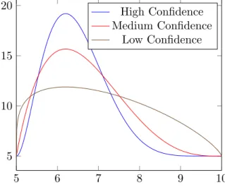
Modified PERT-beta distributions are used throughout the implementations of the FAIR simulation outlined in this thesis. This distribution takes four parameters: minimum, mode, maximum, and confidence. An expert would provide what they believe to be the minimum and maximum values for a particular variable (eg. primary loss magnitude), along with the value that they believe to be most likely (mode) and their confidence in that most likely value [11]. For example, an industry expert with experience in security controls on databases may be tasked with estimating the resistance strength of an organization’s database servers. The expert could decide that the assests have a 33% resistance strength. While this is a very precise estimate, it is very likely wrong. A better course of action is for the expert to provide a range of possible values. In our example, the expert may say they believe the current controls on the database server would provide a resistance strength between 25% and 40%, and they think the most likely resistance strength is 33%. The expert could also say whether they have a high or low confidence in their selection of the most likely (mode) value. These additional parameters allow the expert to better describe their opinion.

5 6 7 8 9 10 5 10 15 20 _{High Confidence} Medium Confidence Low Confidence

Figure 2: PERT distribution PDFs with minimum = 5, mode = 6.2, max = 10, and varying confidence levels (low, medium, and high confidence in the mode).

2.2.1 Beta Distribution

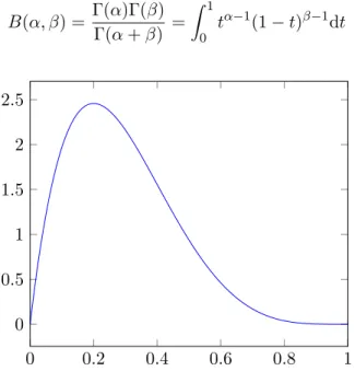
The PERT-beta distribution is a transformation of the standard beta distribution. The standard beta distribution is defined on the range [0,1]. Beta distributions are described by two parametersα, andβ. Figure 3 shows a beta distribution’s probability density function

(17)

(PDF). This function is smooth and continuous between 0 and 1 and it has a value of 0 at both ends of the range. The beta distribution PDF is given in Equation (1) [12].

B(α, β) =Γ(α)Γ(β) Γ(α+β) = Z 1 0 tα−1(1−t)β−1dt (1) 0 0.2 0.4 0.6 0.8 1 0 0.5 1 1.5 2 2.5

Figure 3: The probability density function (PDF) of a beta distribution with α = 2 and

β = 5.

2.2.2 PERT-Beta Distributions

A PERT-beta distribution is the favored distribution for the FAIR model because it allows a risk analyst to specify the desired probability distribution using easy to reason about parameters [10]. These parameters include the minimum (a), mode (b), and maximum

(c). The minimum and maximum parameters describe the range of the distribution, and

the mode specifies the value with the greatest probability of occuring.

The high confidence PERT-beta PDF in Figure 2 and the beta PDF Figure 3 look very similar. They look similar because the PERT-beta distribution is simply a transformation of the beta distribution. A PERT-beta distribution is generated by scaling and shifting a beta distribution along the x-axis such that the range corresponds with the PERT-beta distribution’s minimum and maximum values. Equation (2) illustrates this transformation [13]. The beta function in Equation (1) requires two shape parametersα and β. Equations

(18)

estimated mean,µ. Equation (5) is the estimate of the mean µ of the beta distribution in

terms of the minimum, mode, and maximum parameters [14].

P ERT(a, b, c) =BET A(α, β)∗(c−a) +a (2) where α= (µ−a)(2b−a−c) (b−µ)(c−a) (3) β = α(c−µ) (µ−a) (4) µ= a+ 4b+c 6 (5)

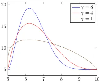
The algorithms in this thesis make use of the modified PERT distribution which is similar to the PERT-beta distribution. The modified PERT distribution takes the three PERT-beta parameters, minimum (a), mode (b), and maximum (c), as well as a confidence in the mode

(γ). The modified PERT distribution has a different approximation of µ which depends

on the new parameterγ. Equation (6) shows the calculation of the mean and it should be

obvious that γ changes the relative weight of the mode in the calculation of the mean. A

lower γ creates a distribution that is flatter and more evenly distributed throughout the

range, while higher values of γ create distributions that are more sharply peaked near the

mode. Figure 4 illustrates the difference in the PDFs with varying confidence levels and the correspondingγ values.

µ= a+γb+c

γ+ 2 (6)

2.3 Sampling from Non-Uniform Distributions

The current implementations of the FAIR simulation generate beta distributions for use in the modified PERT distribution through a method called inverse transform sampling. Inverse transform sampling is a method for generating non-uniform distributions through

(19)

5 6 7 8 9 10 5 10 15 20 _γ _{= 8} γ = 4 γ = 1

Figure 4: Sample PERT distributions with minimum = 5, mode = 6.2, max = 10, and varying confidence levels (low, medium, and high) corresponding to γ = 1, γ = 4, and

γ = 8 respectively.

the transformation of a uniform distribution. For a desired distribution X, let it have a

cumulative density function (CDF) F, then a uniform variate U between 0 and 1 can be

transformed by passing it through the inverse CDF as shown in Equation (7) [15].

X=F−1(U) (7)

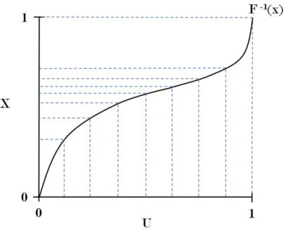
Figure 5 graphically illustrates how inverse transform sampling works. Along theU axis

there are lines uniformly spread across the axis. These extend up to the inverse function

F−1 and extend to theX axis where the lines are no longer evenly spread. They have been transformed into some other distribution that depends on the shape ofF−1.

(20)

Figure 5: Illustration of how inverse transform sampling works by feeding uniform variates into a function F−1 _{to produce non-uniform variates.}

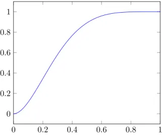
To generate beta distributions using inverse transform sampling, the CDF of the beta distribution must be known. The CDF of the beta distirbution is the regularized incom-plete beta function [12]. This function is given by Equation (9) [16]. Figure 6 shows the corresponding CDF for the PDF in Figure 3. The inverse of the regularized incomplete beta functionIx(α, β) can be used to transform uniform variates into random variates following

a beta distribution. Bx(α, β) = Z x 0 tα−1(1−t)β−1dt 0< x <1 (8) Ix(α, β) = Bx(α, β) B(α, β) (9)

(21)

0 0.2 0.4 0.6 0.8 1 0 0.2 0.4 0.6 0.8 1

Figure 6: The cumulative density function (CDF) of a beta distribution with α = 2 and

(22)

3 Current Sequential Algorithm

3.1 Overview

The current sequential FAIR Monte Carlo simulation implements each node of the FAIR ontology in Figure 1. The algorithm for each node takes in inputs from either the user, or the outputs from nodes below it. This structure makes it quite easy to break the overall simulation down into a few smaller, easier to understand components. These steps are as follows:

1. Vulnerability

2. Primary Loss Magnitude 3. Secondary Loss Magnitude 4. Primary Loss Event Frequency 5. Secondary Loss Event Frequency 6. Risk Exposure

All leaf nodes in the FAIR ontology require user inputs in the form of the modified PERT distribution parameters: minimum, mode, maximum, and confidence. Inputs do not need to be provided for all leaf nodes, instead users may choose to provide inputs for nodes higher in the ontology and have inputs at the lower nodes ignored. This can only be done for the Loss Event Frequency, Threat Event Frequency, and Vulnerability nodes. It should be noted that there are multiple algorithms for the Loss Event Frequency and Vulnerability nodes because of the different sources of inputs.

3.2 Sampling from a PERT-Beta Distribution

Most of the algorithms in the following sections rely on user provided estimates describing the expected values of the FAIR ontology factors that are used in each part of the FAIR model. For each factor the user supplies four values corresponding to the four modified PERT-beta distribution parameters: minimum, mode, maximum, and confidence. The current sequential implementation makes use of the inverse transform method for converting a uniformly distributed variate to a modified PERT-beta distributed variate. Algorithm

(23)

1 takes the PERT descriptors as parameters and computes the inverse incomplete beta function for a random variate U.

Algorithm 1 SamplePERT Inputs: a,b,c,γ,U

Outputs: Random variate from a PERT-beta distribution 1: procedure SamplePERT(a,b,c,γ,U) 2: µ= a+_γγb₊₂+c 3: α= (µ₍−_b₋a)(2_µ₎₍b_c−₋a_a−₎c) 4: β = α₍(_µc₋−_aµ₎) 5: return incbi(α,β,U) ∗(c−a) +a 6: end procedure

The current sequential algorithm is based on the function incbifrom the cephes math library [17]. This function computes the inverse of the regularized incomplete beta function. The regularized incomplete beta function is the CDF of a beta distribution and inverting this function allows a uniform distribution to be mapped to a beta distribution via the inverse transform sampling method.

The incbi function takes as parameters the two shape parametersα and β of the beta

function and a number ywhere 0< y <1. It then finds a number xthat satisfies equation

(10).

Ix(a, b)−y= 0 (10)

At a high level, the function incbiworks by first estimating the inverse by computing the inverse for a normal distribution. This estimated inverse is then used as the starting point for either interval halving (bisection or binary search), or Newton’s method for finding the roots of Equation (10). These methods are executed until a solution for the equation is found, or an error state is reached. For more implementation details, the source code is available online [17].

3.3 Vulnerability

The vulnerability of an asset is the first aspect of a scenario to be calculated. The vulnerability of an asset within a single scenario is the percentage of attacks against it that

(24)

are successful. This percentage can be determined in two ways. The first is by deriving the value from user provided inputs for vulnerability and the second is by estimating it from user provided inputs for Threat Capability and Resistance Strength. Bernoulli trials are used to simulate attacks against the asset. After all iterations, the percentage of successful attacks is taken as the vulnerability of the asset for the scenario.

Direct Mode

When directly calculating vulnerability, the user will provide a minimum, mode, maxi-mum, and confidence value as inputs for Vulnerability. The minimaxi-mum, mode, and maximum values must be in the range [0,1] since the values are probabilities. Algorithm 2 describes how to calculate Vulnerability directly from user inputs.

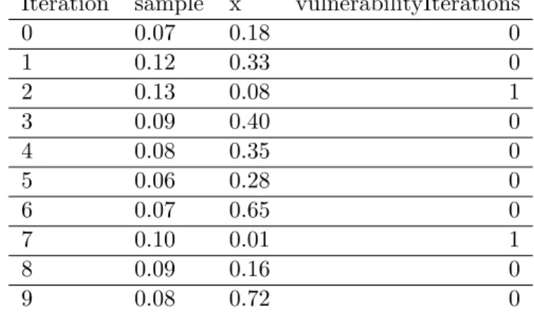
Table 1 contains sample inputs for the direct Vulnerability calculations. As an example, Table 2 contains ten iterations of Algorithm 2. In this example, two of the ten iterations resulted in a 1 being stored in the vulnerabilityIterations array. To complete Algorithm 2 the average of the vulnerabilityIterations array is taken which ends up being 0.2 for this example. This means the asset is vulnerable to 20% of attacks made against it by the threat actor for the scenario.

Algorithm 2 Direct Mode Vulnerability 1: vulnerabilityIterations = new int[iterations] 2: fori=0,...,iterationsdo

3: sample=SamplePERT(vuln.min, vuln.mode, vuln.max, vuln.confidence) 4: x = UniformRandom() 5: if x < samplethen 6: vulnerabilityIterations[i] = 1 7: else 8: vulnerabilityIterations[i] = 0 9: end if 10: end for 11: return average(vulnerabilityIterations)

Minimum Mode Maximum Confidence

Vulnerability 0.05 0.08 0.16 4

(25)

Iteration sample x vulnerabilityIterations 0 0.07 0.18 0 1 0.12 0.33 0 2 0.13 0.08 1 3 0.09 0.40 0 4 0.08 0.35 0 5 0.06 0.28 0 6 0.07 0.65 0 7 0.10 0.01 1 8 0.09 0.16 0 9 0.08 0.72 0

Table 2: Example iterations for Vulnerability estimation in direct input mode.

Derived Mode

When the user chooses to enter inputs for Threat Capability and Resistive Strength they will provide minimum, mode, maximum, and confidence values for both. Once again, the minimum, mode, and maximum values need to be in the range [0,1] since both are probabilities. Threat Capability is the threat actor’s ability to successfully attack the asset. Thus, an input value of 1 for Threat Capability indicates a threat actor is always able to successfully attack an asset, while a value of 0 means the threat actor will never successfully attack the asset. Resistive strength measures the strength of protective controls on the asset. A Resistive Strength of 1 means the controls stop all attacks while a value of 0 means the controls stop no attacks.

Once again Bernoulli trials are used to simulate attacks against the asset, however this time the Resistive Strength and Threat Capability PERT distributions are used as inputs to the Bernoulli trials. Once all simulated attacks have been completed, the asset’s vul-nerability is assigned the percentage of successful attacks. Algorithm 3 details the steps involved in calculating Vulnerability with this method.

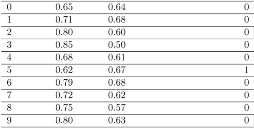
Table 3 contains sample inputs for Threat Capability and Resistive Strength, and in Table 4 examples are provided for Algorithm 3 with ten iterations using the sample inputs. As shown in the attackResult row, only one of the ten iterations saw a successful attack against the asset. Calculating the average of the attackResult column gives the estimated Vulnerability of the asset for the scenario. In this case, the average is 0.10, indicating the

(26)

asset is vulnerable to 10% of attacks. Algorithm 3 Derived Mode Vulnerability

1: attackResults = new int[iterations] 2: fori=0,...,iterationsdo

3: resistance = SamplePERT(rs.min, rs.mode, rs.max, rs.confidence)

4: threatCapability = SamplePERT(tcap.min, tcap.mode, tcap.max, tcap.confidence) 5: if threatCapability < resistancethen

6: attackResults[i] = 1 7: else 8: attackResults[i] = 0 9: end if 10: end for 11: return average(attackResults)

Threat Capability (tcap) 0.45 0.65 0.70 8

Resistance Strength (rs) 0.60 0.70 0.90 4

Table 3: Sample inputs for Vulnerability estimation in derived mode.

Iteration resistance threatCapability attackResults

0 0.65 0.64 0 1 0.71 0.68 0 2 0.80 0.60 0 3 0.85 0.50 0 4 0.68 0.61 0 5 0.62 0.67 1 6 0.79 0.68 0 7 0.72 0.62 0 8 0.75 0.57 0 9 0.80 0.63 0

Table 4: Example iterations for Vulnerability estimation in derived mode.

3.4 Primary Loss Magnitude

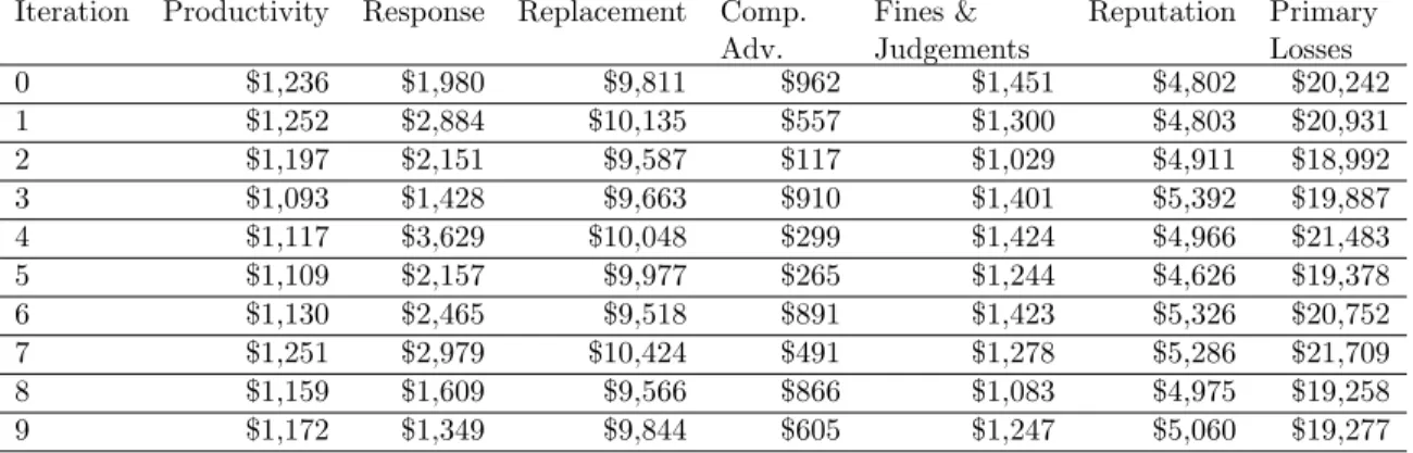
The primary losses for a scenario are the losses that are experienced as a direct result of a successful attack against the asset. There are 6 forms of loss and they are: productivity costs, response costs, replacement costs, competitive advantage losses, fines and judgements, and reputation losses. Users provide inputs for each of the six forms of loss. The input for each form of loss will contain a minimum, mode, maximum, and a confidence value.

(27)

Table 5 contains sample inputs for calculating Primary Loss and Algorithm 4 describes how these inputs are used to produce the output for this step. The inputs for each of the six forms of loss have a minimum, mode, maximum, and confidence. The output from Algorithm 4 is an array of primary loss values. Each of these values represents a potential loss that can be experienced because of an attack. This array of values will be used in later steps.

Algorithm 4 Primary Loss

1: primaryLosses = new double[iterations] 2: set all primaryLosses to 0

3: fori=0,...,iterationsdo 4: iterationLosses = 0

5: for all f in formsOfLossdo

6: iterationLosses += SamplePERT(f.min, f.mode, f.max, f.confidence) 7: end for

8: primaryLosses[i] = iterationLosses 9: end for

10: return primaryLosses

Productivity $1,000 $1,233 $1,275 1

Response $1,000 $1,525 $4,500 8

Replacement $9,500 $9,650 $10,500 8

Competitive Advantage $50 $857 $999 8

Fines & Judgements $1,000 $1,250 $1,500 4

Reputation $4,500 $5,200 $5,500 4

Table 5: Sample inputs for calculating primary losses at each iteration.

Iteration Productivity Response Replacement Comp. Adv. Fines & Judgements Reputation Primary Losses 0 $1,236 $1,980 $9,811 $962 $1,451 $4,802 $20,242 1 $1,252 $2,884 $10,135 $557 $1,300 $4,803 $20,931 2 $1,197 $2,151 $9,587 $117 $1,029 $4,911 $18,992 3 $1,093 $1,428 $9,663 $910 $1,401 $5,392 $19,887 4 $1,117 $3,629 $10,048 $299 $1,424 $4,966 $21,483 5 $1,109 $2,157 $9,977 $265 $1,244 $4,626 $19,378 6 $1,130 $2,465 $9,518 $891 $1,423 $5,326 $20,752 7 $1,251 $2,979 $10,424 $491 $1,278 $5,286 $21,709 8 $1,159 $1,609 $9,566 $866 $1,083 $4,975 $19,258 9 $1,172 $1,349 $9,844 $605 $1,247 $5,060 $19,277

(28)

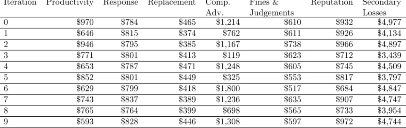
3.5 Secondary Loss Magnitude

The Secondary Loss Magnitude for a scenario is broken down into the same six forms of loss as Primary Loss Magnitude. Secondary losses are experienced incidentally to primary losses. An important distinction between primary and secondary losses is that primary losses will always occur after a successful attack, while secondary losses have a chance of not occurring after a successful attack. In this step of the process, only the potential secondary losses are calculated. The Secondary Loss Event Frequency step will determine if the secondary losses actually occur.

Users provide inputs for each of the six forms of secondary loss. The calculated values for each form are summed to give the total Secondary Loss Magnitude. Algorithm 5 details the steps required to calculate Secondary Loss Magnitude from the user’s inputs.

The output from Algorithm 5 is an array of secondary loss magnitudes, one for each iteration. This array is stored for later use in calculating the total loss magnitude for each iteration. Table 7 gives sample inputs for secondary loss magnitude estimation and Table 8 gives an example of the calculations for several iterations of Algorithm 5.

Algorithm 5 Secondary Loss Magnitude 1: secondaryLosses = new double[iterations] 2: set all secondaryLosses to 0

3: fori=0,...,iterationsdo 4: iterationLosses = 0

5: for all f in formsOfLossdo

6: iterationLosses += SamplePERT(f.min, f.mode, f.max, f.confidence) 7: end for

8: secondaryLosses[i] = iterationLosses 9: end for

10: return secondaryLosses

Productivity $500 $650 $1,000 8

Response $750 $800 $850 1

Replacement $325 $450 $500 8

Competitive Advantage $0 $1,000 $2,000 4

Fines & Judgements $500 $550 $800 8

Reputation $600 $900 $1,000 1

(29)

Iteration Productivity Response Replacement Comp. Adv. Fines & Judgements Reputation Secondary Losses 0 $970 $784 $465 $1,214 $610 $932 $4,977 1 $646 $815 $374 $762 $611 $926 $4,134 2 $946 $795 $385 $1,167 $738 $966 $4,897 3 $771 $801 $413 $119 $623 $712 $3,439 4 $653 $787 $471 $1,248 $605 $745 $4,509 5 $852 $801 $449 $325 $553 $817 $3,797 6 $629 $799 $418 $1,800 $517 $684 $4,847 7 $743 $837 $389 $1,236 $635 $907 $4,747 8 $765 $764 $399 $698 $565 $733 $3,954 9 $593 $828 $446 $1,308 $597 $972 $4,744

Table 8: Example iterations for secondary losses estimation.

3.6 Primary Loss Event Frequency

Primary Loss Event Frequency (PLEF) calculates the number of loss events per year. There are three ways to calculate PLEF. The first relies on the user directly entering inputs for the Loss Event Frequency node. In this case, Vulnerability does not need to be calculated. The second method is used if the user enters inputs for the Threat Event Frequency node. This will utilize the calculated Vulnerability for the scenario and the Threat Event Frequency inputs to calculate the PLEF. Finally, the user can enter inputs for Contact Frequency and Probability of Action nodes. These two inputs will be used to calculate Threat Event Frequency, which will then be used with the calculated Vulnerability to determine Loss Event Frequency.

Direct Mode

When calculating PLEF directly, the user provides only inputs for the PLEF node. Algorithm 6 goes over the steps required to calculated PLEF and Table 9 contains sample inputs. Table 10 provides sample iterations and in the last column of the table, the number of primary loss events for each iteration is recorded. This number indicates the number of loss events that occurred within a year.

Primary Loss Event Frequency 0.1 1.5 9.0 4

(30)

Algorithm 6 Primary Loss Event Frequency - Direct Mode 1: primaryLEFs = new int[iterations]

2: fori=0,...,iterationsdo

3: sampledPLEF = SamplePERT(plef.min, plef.mode, plef.max, plef.confidence) 4: r = Random.NextDouble() 5: iterationPLEF = 0 6: if sampledPLEF< 1then 7: if r <sampledPLEF then 8: iterationPLEF = 1 9: end if 10: else 11: major = floor(sampledPLEF) 12: minor = sampledPLEF - major 13: if r <minorthen 14: iterationPLEF = major + 1 15: else 16: iterationPLEF = major 17: end if 18: end if 19: primaryLEFs[i] = iterationPLEF 20: end for 21: return primaryLEFs

Iteration sampledPLEF r major minor iterationPLEF

0 1.27 0.29 1 0.27 1 1 1.72 0.70 1 0.72 2 2 4.00 0.03 4 0.00 4 3 3.96 0.97 3 0.96 3 4 1.58 0.18 1 0.58 2 5 6.02 0.51 6 0.02 6 6 7.38 0.19 7 0.38 8 7 0.36 0.52 - - 0 8 5.22 0.69 5 0.22 5 9 2.77 0.31 2 0.77 3

Table 10: Example iterations for Priamry Loss Event Frequency estimation.

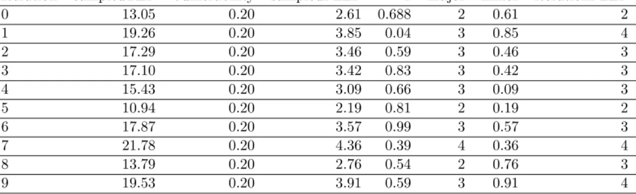
Derived from Threat Event Frequency and Vulnerability

PLEF can be determined when the user provides inputs for the Threat Event Frequency node and inputs for calculating Vulnerability. The method in which PLEF is determined is very similar to the previously described method. The only change to the algorithm is on line 4 where sampled PLEF is calculated from threat event frequency and vulnerability.

(31)

Vulnerability has already been calculated at this point and is a single probability in the range [0,1]. Table 11 contains sample inputs for Algorithm 7. Table 12 contains values for ten iterations of Algorithm 7.

Algorithm 7 Primary Loss Event Frequency - TEF/VULN Mode 1: primaryLEFs = new int[iterations]

3: sampledTEF = SamplePERT(tef.min, tef.mode, tef.max, tef.confidence) 4: sampledPLEF = sampledTEF * Vulnerability

5: r = Random.NextDouble() 6: iterationPLEF = 0 7: if sampledPLEF< 1then 8: if r <sampledPLEF then 9: iterationPLEF = 1 10: end if 11: else 12: major = floor(sampledPLEF) 13: minor = sampledPLEF - major 14: if r <minorthen 15: iterationPLEF = major + 1 16: else 17: iterationPLEF = major 18: end if 19: end if 20: primaryLEFs[i] = iterationPLEF 21: end for 22: return primaryLEFs

Threat Event Frequency 10 14 28 4

Vulnerability 0.20

Table 11: Sample inputs for estimation of Primary Event Loss Frequency from Threat Event Frequency and Vulnerability.

(32)

Iteration sampledTEF Vulnerability sampledPLEF r major minor iterationPLEF 0 13.05 0.20 2.61 0.688 2 0.61 2 1 19.26 0.20 3.85 0.04 3 0.85 4 2 17.29 0.20 3.46 0.59 3 0.46 3 3 17.10 0.20 3.42 0.83 3 0.42 3 4 15.43 0.20 3.09 0.66 3 0.09 3 5 10.94 0.20 2.19 0.81 2 0.19 2 6 17.87 0.20 3.57 0.99 3 0.57 3 7 21.78 0.20 4.36 0.39 4 0.36 4 8 13.79 0.20 2.76 0.54 2 0.76 3 9 19.53 0.20 3.91 0.59 3 0.91 4

Table 12: Example iterations for estimating Primary Loss Event Frequency from Threat Event Frequency and Vulnerability.

Derived from Contact Frequency, Probability of Action, and Vulnerability The final method of estimating PLEF is by estimating Threat Event Frequency from Contact Frequency and Probability of Action, and then using that result along with the scenario vulnerability, to estimate PLEF. Algorithm 8 outlines the steps involved in esti-mating PLEF in this case. Table 13 lists sample inputs for this step and Table 14 contains example values for ten iterations.

Contact Frequency 500 600 800 8

Probability of Action 0.10 0.25 0.30 4

Vulnerability 0.20

Table 13: Sample inputs for estimation of Primary Loss Event Frequency from Contact Frequency, Probability of Action, and Vulnerability

Iteration sampledPoA sampledCF Vulnerability sampledPLEF r major minor iterationPLEF 0 0.23 533.4 0.20 24.54 0.74 24 0.54 24 1 0.25 613.4 0.20 30.67 0.50 30 0.67 31 2 0.21 628.7 0.20 26.41 0.83 26 0.41 26 3 0.24 727.0 0.20 34.90 0.88 34 0.90 35 4 0.38 623.3 0.20 34.90 0.65 34 0.90 35 5 0.14 543.2 0.20 15.21 0.44 15 0.21 15 6 0.25 629.4 0.20 30.21 0.18 30 0.21 31 7 0.26 620.5 0.20 32.27 0.09 32 0.27 33 8 0.29 703.4 0.20 40.80 0.30 40 0.80 41 9 0.21 619.8 0.20 26.03 0.35 26 0.03 26

Table 14: Example iterations for estimating Primary Loss Event Frequency from Probability of Action, Contact Frequency, and Vulnerability.

(33)

Algorithm 8 Primary Loss Event Frequency - CF/POA/VULN Mode 1: primaryLEFs = new int[iterations]

3: sampledPoA = SamplePERT(poa.min, poa.mode, poa.max, poa.confidence) 4: sampledCF = SamplePERT(cf.min, cf.mode, cf.max, cf.confidence)

5: sampledPLEF = sampledPoA * sampledCF * Vulnerability 6: r = Random.NextDouble() 7: iterationPLEF = 0 8: if sampledPLEF< 1then 9: if r <sampledPLEF then 10: iterationPLEF = 1 11: end if 12: else 13: major = floor(sampledPLEF) 14: minor = sampledPLEF - major 15: if r <minorthen 16: iterationPLEF = major + 1 17: else 18: iterationPLEF = major 19: end if 20: end if 21: primaryLEFs[i] = iterationPLEF 22: end for 23: return primaryLEFs

(34)

3.7 Secondary Loss Event Frequency

Secondary Loss Event Frequency determines how often secondary losses are experienced when there has been a threat event. This is calculated directly from user provided inputs for this node. Unlike Primary Loss Events, Secondary Loss Events do not always happen when there is a successful attack against an asset. Every loss event will be a Primary Loss Event, and a subset of those events will also include secondary loss events. Due to this dependence on the PLEF, Algorithm 9 requires the output from that step. Algorithm 9 describes the steps involved in estimating Secondary Loss Event Frequency and Table 15 provides sample inputs.

The last row of Table 16 is the number of secondary loss events per iteration. It should be clear that the secondary loss event frequency will always be equal to or less than the PLEF. This resultant array of values is stored for use in the next step.

Algorithm 9 Secondary Loss Event Frequency 1: secondaryLEFs = new int[iterations]

2: fori=0,...,iterationsdo 3: secondaryLEFs[i] = 0

4: for j=0,...,primaryLEFs[i]do

5: sampledSLEF = SamplePERT(slef.min, slef.mode, slef.max, slef.confidence) 6: r = Random.NextDouble() 7: if r <sampledSLEF then 8: secondaryLEFs[i]++ 9: end if 10: end for 11: end for 12: return secondaryLEFs

Secondary Loss Event Frequency 0.12 0.21 0.30 8

(35)

Iteration PLEF sampledSLEF r sampledSLEF r sampledSLEF r SLEF 0 3 0.21 0.50 0.29 0.59 0.25 0.59 0 1 2 0.27 0.54 0.13 0.15 - - 0 2 3 0.22 0.14 0.14 0.20 0.20 0.13 2 3 1 0.17 0.33 - - - - 0 4 3 0.22 0.19 0.17 0.52 0.16 0.42 1 5 3 0.24 0.77 0.13 0.05 0.27 0.40 1 6 1 0.19 0.30 - - - - 0 7 1 0.21 0.86 - - - - 0 8 1 0.18 0.60 - - - - 0 9 2 0.21 0.85 0.21 0.62 - - 0

Table 16: Example iterations for calculating secondary loss event frequencies.

3.8 Risk Exposure

The last step of the FAIR Monte Carlo simulation is to pull together the outputs from previous steps to produce the overall risk exposure for the current scenario. To complete this the output arrays from Primary Loss Event Frequency, Secondary Loss Event Frequency, Primary Loss Magnitude, and Secondary Loss Magnitude are needed. There are no direct user inputs for this step of the process. Algorithm 10 details the steps to calculate the Risk Exposure for the scenario and Table 17 contains example iterations.

Algorithm 10Risk Exposure

1: riskExposure = new double[iterations] 2: fori=0,...,iterationsdo

3: primaryExposure = primaryLossMagnitude[i] * primaryLossEventFrequency[i] 4: secondaryExposure = secondaryLossMagnitude[i] * secondaryLossEventFrequency[i] 5: riskExposure[i] = primaryExposure + secondaryExposure

6: end for

(36)

Iteration PLEF SLEF PLM SLM Risk Exposure 0 3 0 $20,242 $4,977 $60,726 1 2 0 $20,931 $4,134 $41,862 2 3 2 $18,992 $4,897 $66,770 3 1 0 $19,887 $3,439 $19,887 4 3 1 $21,483 $ 4,509 $68,958 5 3 1 $19,378 $4,847 $61,931 6 1 0 $20,753 $4,847 $20,753 7 1 0 $21,709 $4,747 $21,709 8 1 0 $19,258 $3,954 $19,258 9 2 0 $19,277 $4,744 $38,664

(37)

4 Parallel Algorithms

For this thesis, the generation of samples from PERT-beta distributions and the FAIR Monte Carlo simulation were implemented for the GPU using NVIDIA’s CUDA technology. How these were parallelized is explained throughout the following section.

4.1 Sampling from PERT-Beta Distributions

The sequential algorithm for generating random samples from a PERT-Beta distribution relies heavily on the inverse transformation method to transform uniformly distributed values in the range [0,1] to PERT-beta distributed values. For the parallel implementation, rather than computing each PERT-Beta sample as its needed, all the samples for a each step are generated all at once by many parallel threads. An array of uniform samples is generated on the GPU using a CUDA library called cuRAND that provides a simple method for generating uniform distributions on the GPU. The GPU function, or kernel, that performs the inverse transform grabs a number from the uniform array, transforms it, then places it in the same position of an output array. Three different methods were implemented to perform this transformation.

Parallel Execution of incbi

The first of these methods executes theincbifunction on the GPU for every value that is transformed. Algorithm 11 outlines the process for transforming an array of uniformly distributed valuesU to a PERT-Beta distributed array. This algorithm has the benefit that

the transformed values will be more accurate than the transformed values from Algorithms 12 and 13. The performance and accuracy tradeoffs are later presented and discussed in the results section.

Algorithm 11 is very simple. However, in the CUDA architecture, this solution is not optimal. The incbi function is a large and complex function with many divergent code paths. Executing such code is not optimal in CUDA due to a phenomenon called thread divergence. Thread divergence occurs in CUDA because not all threads execute completely independently of one another. CUDA runs groups of 32 threads together as a single warp.

(38)

Algorithm 11Parallel incbi

LetU be an array ofnuniformly distributed numbers in the range [0,1]. Lettransf ormed be an array of sizen.

1: procedure ParallelIncbi(U,n,α,β)

2: for nparallel threads with threadIdsifrom 0 to n−1 do 3: InverseIncompleteBeta(i,U,α,β,transf ormed) 4: end forreturn transf ormed

5: end procedure

6: procedure InverseIncompleteBeta(i,U,α,β,output)

7: output[i] =incbi(α,β,U[i])

8: end procedure

All running threads within a warp execute the same instructions at the same time. If threads within a warp should be executing a different set of instructions, such as during an if/else statement, those threads will execute their instructions sequentially. This means the threads executing the first part of the path will execute while the threads in the other part will sit idle. Once the running threads have completed the first part, the second group of threads will execute their instructions while the first threads sit idle. As shown by Bialas and Strzelecki thread divergence can severly impact performance, potentially increasing runtime up to 32x when all threads in a warp are executing different instructions [18].

There are methods that can be employed to reduce the amount of thread divergence within warps. These methods range from compile-time analysis and optimization of warp task assignment [19] to consideration of tradeoffs of error tolerance for less control diver-gence and improved parallelism [20]. It is the latter method that this thesis focuses on for improving the inverse transformation of large arrays of uniformly distributed numbers to beta distributions.

Lookup Table based Inverse Transform Sampling

A method for inverse transformation is described by Nagli˘c et al. where a table was used to store precalculated values for difficult to compute light propagation phase functions. In simulations the table was then used to lookup the precomputed values and improve the performance of the simulation [21]. This thesis presents a similar method for the transfor-mation of uniform samples by an inverse incomplete beta lookup table. This transfortransfor-mation

(39)

is composed of two steps: an initial precompute step and a transformation step.

In the first step of the lookup table based inverse transform, a lookup table for the inverse of the incomplete beta function is produced. This makes use of the cumulative density function (CDF) of the beta distribution, which is the regularized incomplete beta function (9) [12]. The values of the lookup table will be computed fromIx(α, β) =y where,

for each index in the lookup table, the index divided by the table size is used as the value ofxand the resultyis stored at the index. Algorithm 12 outlines this process for a parallel

environment where each thread calculates a different index of the lookup table. Calculating

Ix(a, b) in its integral form is a difficult computational task that can be made simpler by

using the continued fraction form shown in Equation (11) [16]. The continued fraction is computed out to d300 or until the result has matched or exceeded the precision of the

machine. Ix(a, b) = xa(1−x)b aB(a, b) ₁ 1+ d1 1+ d2 1+ d3 1+... (11) where d2m= m(b−m)x (a+ 2m−1(a+ 2m) (12) d2m+1= (a+m)(a+b+m)x (a+ 2m)(a+ 2m+ 1) (13)

In the second step of the lookup table based inverse transform sampling, a large array of uniform variates (U) is transformed in parallel. Each thread is tasked with transforming

a single value y from U. This is done by searching the lookup table for an index m such

that the value at m is less thany and the value atm+ 1 is greater thany. The algorithm

then interpolates the values at the indices m and m+ 1 to produce an approximation

to the inverse incomplete beta function for y. Algorithm 13 describes this process. The

procedure ParallelApproximatePERTBetaTransform is the entry point for Algorithm 13. Two methods of searching the lookup table were implemented for this thesis: a linear scan and a binary search.

(40)

Algorithm 12Initialize Inverse Lookup Letlookupbe an array of size n+ 1.

1: procedure ParallelInitializeInverseLookup(n,α,β,lookup)

2: for nparallel threads with threadIdsifrom 0 to ndo 3: _{InitializeInverseBetaLookup}(i,n,α,β,lookup) 4: end for

5: end procedure

6: procedure InitializeInverseBetaLookup(threadIdx,n,α,β,lookup)

7: x=threadIdx/n . Determine the value of x to computeIx(α, β) 8: y =Ix(α, β) .Computed using the continued fraction shown in equation (11) 9: lookup[threadIdx] =y

10: end procedure

Algorithm 13Parallel Inverse Beta Transform

Transforms an array U of n uniformly distributed numbers in the range [0,1] into ap-proximately beta distributed numbers.

1: procedure ParallelApproximatePERTBetaTransform(U, min, max, lookup,

lookuplength,n)

2: Let transf ormedbe an array of size n.

3: for nparallel threads with threadIdsifrom 0 to n−1 do

4: _{InversePERTBeta}(i,U,transf ormed,lookup,lookuplength,min,max) 5: end for

6: return transf ormed

7: end procedure

8: procedure InversePERTBeta(threadIdx, U, output, lookup, lookuplength, min,

max) 9: y =U[threadIdx] 10: x0= 0.0 11: x1= 0.0 12: l= 0 13: r =lookuplength−1 14: m

15: Perform a search for the index m in lookup such that lookup[m] ≤ y and y ≤

lookup[m+ 1]

16: x=Interpolate(lookup[m+ 1], x0, lookup[m], x1, y)

17: output[threadIdx] =min+ (max−min)∗x . Scales the values to the PERT min and max parameters

18: end procedure 19: procedure Interpolate(x0,y0,x1,y1,x) 20: y =y0+ (y1−y0) x−x0 x1−x0 21: end procedure

(41)

4.2 Parallelizing the FAIR Simulation

The previously described inverse table lookup transform method was applied to a par-allelized version of the FAIR Simulation described in Section 3. This necessitated the parallelization of the FAIR simulation algorithms. The majority of the algorithms have an outer for loop that can be easily parallelized. This make parallelization fairly straight forward since each thread on the GPU can be assigned to do the work for a single iteration of the loop. This is possible because each iteration is independent of all other iterations.

Each algorithm of the FAIR simulation was implemented to take in arrays with an element for each iteration. Each input array is filled with samples from a PERT-Beta distribution described by the user inputs, or outputs from another part of the simulation. Each thread is assigned a unique integer id. This id is used to index the input arrays and access the values for the simulation. The thread calculates the result for the current algorithm being executed, and uses the id to store that result in the output array. Figure 7 illustrates the parallelization of the FAIR simulation algorithms.

Figure 7: Parallel model for each FAIR simulation algorithm. Each thread performs the work that would have been in the for loop of the sequential algorithms.

(42)

This pattern works for the majority of the FAIR simulation algorithms with the exception of the Vulnerability and SLEF algorithms. These require some work before or after the parallelized portions in order to work.

For the Vulnerability algorithms, an average needs to be calculated from the resulting Vulnerability array. For simplicity, the average of the Vulnerability array is calculated on the CPU. It is possible to accelerate the average calculation using the GPU to perform the summation work in calculating the average of the array. The summation can be implemented as an inclusive scan as described by Harris [22]. However, that will be left for future work. In the sequential algorithm for SLEF, samples from the SLEF distribution are taken for each primary loss event in each iteration. The algorithm therefore requires an array of SLEF samples equal in length to the sum of all primary loss events. Once again, for simplicity, the summation of the primary loss events is performed on the CPU, but could be moved to the GPU. This was computed as a prefix scan with each prefix sum stored in an array for use by the parallel Secondary Loss Event Algorithm. This array is the same length as the primary loss event array, and each value is an offset into the SLEF samples array where each thread can begin using sampled SLEF values. This method prevents different threads from accessing the same index and double sampling some values, preserving the PERT-Beta distribution. Algorithm 14 is executed in each thread in the parallel version of Secondary Loss Event Frequency.

Algorithm 14Secondary Loss Event Frequency Kernel

1: procedure SLEFKernel(threadIdx, outputs, plef, slef, uniform, slefOffsets)

2: secondaryLossEvents = 0

3: primaryLossEvents = plef[threadIdx] 4: for i=0 ... primaryLossEventsdo

5: sampledSLEF = slef[slefOffsets[threadIdx] + i] 6: r = uniform[slefOffsets[threadIdx] + i] 7: if r <sampledSLEF then 8: secondaryLossEvents++ 9: end if 10: end for 11: outputs[threadIdx] = secondaryLossEvents 12: end procedure

(43)

5 Results

5.1 Inverse Regularized Incomplete Beta Comparison

In order to verify the lookup table based approximations for the inverse incomplete beta function can be used to perform inverse transform sampling, it needs to be shown that the precomputed values in the tables approximate the inverse incomplete beta function. This was done by calculating the inverse incomplete beta function for 10,000 numbers evenly spaced numbers between 0 and 1. Figure 8 shows scatter plots of the results of this process. The upper plot shows the values produced by the lookup table with a size of 8. The points in this plot show a function that is clearly not smooth, and is nowhere near as smooth as the one produced by theincbifunction. As the size of the lookup table increases, the plot appears to become more smooth. The middle plot of Figure 8 is produced by a lookup table with 4,096 entries. It appears just as smooth as the plot produced byincbiand appears to match it very well. The difference in time to initialize lookup tables of different sizes was negligible for all tested table sizes.

In Figure 9, the distribution of errors between the interpolated lookup table values and the values produced by incbi are shown for various lookup table sizes. Errors were calculated by generating 100,000 random numbers between [0,1] and computing the inverse using the lookup table and incbi. The absolute difference between the two values was calculated and plotted on the histogram. It can be clearly seen that the smaller lookup tables had many more larger errors. This was to be expected after looking at the inverse CDFs produced by the smaller lookup table in Figure 8. At the table sizes of 2048 and 4096, the distributions of errors is in a very narrow range around 0. This suggests that increasing the table size further would be of diminishing benefit. Indeed, looking at the minimum, mean, and maximum recorded errors for the lookup table sizes in Table 18, the average error is smaller than 10−7 at those lookup table sizes. Within the FAIR model an error of 10−7 would correspond with a 1 in 10 million year loss event or would be the difference between a loss of $10,000,000 or $10,000,001. There is no requirement in the application for such accuracy, so a lookup table of 4,096 elements provides more than enough accuracy.

(44)

Figure 8: Plots of the interpolated values from the inverse lookup table for a beta distribu-tion with α = 5 andβ = 8. The top two plots are generated from the inverse tables with sizes of 8 and 4096. The bottom plot shows the inverse values computed by incbi.

(45)

Figure 9: Distributions of absolute errors in the lookup based methods compared to the

(46)

Lookup Table Size Minimum Error Average Error Maximum Error 4 5.78×10−9 2.65×10−2 1.49×10−1 8 1.29×10−9 6.95×10−3 7.56×10−2 16 8.96×10−11 1.77×10−3 2.83×10−2 32 6.72×10−12 4.44×10−4 1.45×10−2 64 4.53×10−13 ₁_.₁₁_×₁₀−4 ₇_.₂₄_×₁₀−3 128 6.74×10−14 ₂_.₇₈_×₁₀−5 ₁_.₇₄_×₁₀−3 256 1.82×10−14 6.95×10−6 5.53×10−4 512 4.55×10−15 1.74×10−6 1.29×10−4 1024 1.11×10−16 4.34×10−7 2.87×10−5 2048 6.66×10−16 1.09×10−7 9.35×10−6 4096 1.11×10−16 2.71×10−8 2.11×10−6 8192 0.00 6.78×10−9 5.31×10−7 16384 0.00 1.70×10−9 2.00×10−7 32768 0.00 4.24×10−10 4.33×10−8 65536 0.00 1.06×10−10 9.06×10−9

Table 18: The error in calculating the inverse of the regularized incomplete beta function using the method in algorithm 13 compared to the cephes implementation of incbi. Fore-ach table size, 1,000,000 uniformly random numbers were transformed and the minimum, average, and maximum errors were recorded.

Figure 10: Graph generated from Table 18 of the absolute error of the lookup table based methods for calculating the inverse incomplete beta for various sizes of lookup tables.

(47)

5.2 Performance of the Lookup Table Based Inverse Transforms

One of the most common methods of comparing sequential and parallel implementation performance is by using a metric called speed-up. Speed-up is defined as the ratio of the runtime of the sequential implementation to the runtime of the parallel implementation withp processors as shown in Equation (14).

T(n,1)

T(n, p) (14)

Table 19 and Figure 11 show the speed-ups for the parallel implementations of inverse transforms described in Algorithms 11 and 13. The Exact Calc. method, which calculates

incbiin each thread acheives a maximum speedup of 31x over the sequential implementa-tion. Both lookup table based implementations improve upon this significantly. The lookup method using a linear search of the lookup table acheives a maximum speedup of 169x and the lookup with a binary search acheives an even greater speedup of 390x. Interestingly, looking at Figure 11, the Exact Calc. implementation doesn’t seem to be increasing its speed-up after about 100,000 samples, while binary search based Lookup is still increasing its speed-up at 10,000,000 samples.

Generated Samples Exact Calc. Lookup (Linear search) Lookup (Binary Search)

1 0.0001 0.0046 0.0084 10 0.0406 0.0293 0.0394 100 0.378 0.258 0.373 1,000 2.09 2.66 3.71 10,000 12.2 18.0 18.6 100,000 25.2 86.7 134 1,000,000 29.0 169 327 10,000,000 31.1 159 390

Table 19: The speed-up of three methods for calculating inverse transforms in CUDA for various sample sizes. The Exact Calc. column is the speed-up of Algorithm 11 over the sequential implementation. The two Lookup columns present speed-ups of Algorithm 13 with either a linear or binary search compared to the sequential implementation.

(48)

Figure 11: Graph of the values from Table 19.

Another factor in the performance of the Lookup table based inverse transforms is the size of the lookup table. Clearly, a large lookup table will take longer, on average to search for a particular value. Linear searches have a runtime of O(n) while binary searched have an average runtime of O(logn). Therefore it is expected that the binary search based Lookup transform should have better performance than the linear search lookup transform for large lookup table sizes. Indeed, in experimentation, this expectation appears to hold true. Table 20 shows the speed-ups for the two lookup transforms for increasing lookup table sizes. Each test transformed 1,000,000 samples. For lookup tables larger than 64 elements, the binary search is faster than the linear search. Infact, the binary search based lookup transform only lost about 15% of its performance while the table size increased a factor of 214.

(49)

Lookup Table Size Lookup (Linear search) Lookup (Binary Search) 4 342 328 8 341 338 16 343 321 32 325 319 64 310 321 128 299 313 256 259 314 512 203 302 1024 143 300 2048 88.3 301 4096 51.2 311 8192 27.7 302 16384 15.1 305 32768 7.95 297 65536 4.10 278

Table 20: Speed-up of lookup table based inverse transforms with increasing lookup table sizes.

Figure 12: The speed-ups from Table 20 plotted against table size.

5.3 Quality of Generated Beta Distributions

The lookup table based inverse transform methods have good performance compared to the sequential based implementation, and the approximations to the inverse incomplete

(50)

beta function appear to be accurate for sufficiently large lookup tables. This implies that the methods will produce accurate beta distributions. Figure 13 shows distributions that result from transforming uniform distributions of 1,000,000 samples with various lookup table sizes.

Figure 13: Example beta distributions produced by the Lookup Table Inverse Transfor-mation method for various sizes of the lookup table. The lowest graph is a distribution produced by theincbi function. Distributions were produced with 1,000,000 samples.

(51)

evident in the histograms of the 16 and 32 element lookup tables. As the size of the table increases, these steps become smaller until they become lost in the random noise. The steps occur because of the linear interpolation when performing the transformation. The top plot in Figure 8 shows these linear segments. A linear inverse CDF simply causes a linear transformation of a uniform distribution. This is why each step is flat in the smaller lookup table sizes. At a lookup table size of 256, the steps are no longer noticable.

While a visual comparison of the histograms of the generated distributions suggests that the distributions generated using larger lookup tables are very similar to the distributions produced by the sequential methods, statistical tests are needed to verify this. There are many statistical tests that can compare sampled distributions, but the most fitting is the Kolmogorov-Smirnov (K-S) test. This test finds the maximum distance between the cumulative density function of a reference distribution and the cumulative density function of the experimental data [23]. This test assumes that the null hypothesis is the experimental samples are drawn from the reference distribution. When a confidence level ofαis used the

null hypothesis can be rejected when the p-value of the test is below 1−α. For example, if the p-value for the test was 0.15 andα = 0.95, then the null hypothesis could not be rejected

and it is possible for the samples to be from the reference distribution. If the p-value was 0.01, the null hypothesis could be rejected and it could be said the samples were not pulled from the reference distribution.

Table 21 contains the test statistic and p-value for beta distributions generated from the inverse lookup table method. These statistics were calculated using the python scipy library’s stats.kstest function for the K-S test calculations, and stats.beta for the reference CDF [24]. Assuming a confidence value of 95%, and according to the p-values in Table 21 the null hypothesis could be rejected for the distributions generated from lookup tables with 64 or less elements. This means the diference between the CDF of the generated distribution and the reference CDF were statistically significant and that the inverse lookup table method would need more than 128 elements to generate beta distributions that are close to the reference beta CDF. This reaffirms the earlier conclusion that larger lookup tables produce distributions that more closely match the reference implementation. In particular, lookup tables must be larger than 128 elements.

(52)

Lookup Table Size K-S Test Statistic P-Value 16 0.0137 6.69×10−163 32 0.0042 1.22×10−15 64 0.0014 0.047 128 0.0008 0.568 256 0.0007 0.652 512 0.0008 0.570 1024 0.0010 0.223 2048 0.0008 0.492 4096 0.0009 0.455

Table 21: Kolmogorov-Smirnov test statistics for beta distributions generated by the inverse lookup table method.

5.4 Comparison of the GPU Accelerated FAIR Monte Carlo Simulation to the Sequential Simulation

In Section 4, a set of algorithms was described that parallelize the sequential FAIR Monte Carlo simulation algorithms described in Section 3. These algorithms were implemented for the GPU using NVIDIA’s CUDA technology. Since these simulations rely heavily on the generation of beta distributions and it was shown that the inverse table lookup with binary search resulted in speedups up to 390x over the sequential versions, large perfor-mance improvements can be expected. Because of its excellent perforperfor-mance and acceptable accuracy, the lookup table with binary search was used to generate beta distributions in the parallel FAIR Monte Carlo simulation produced for this research. A lookup table with 4,096 elements was used in this FAIR simulation of the high accuracy shown with tables of that size. The following section analyzes the performance and accuracy of the parallel implementation for three distinct FAIR Scenarios.

All three scenarios have unique inputs which are provided in Appendix B in Tables 29, 30, and 31. These inputs were selected in order to test the different sets of FAIR factors that can be used to describe a FAIR scenario. Scenario 1 (Table 29) uses direct mode Vulnerability calculations and estimates Loss Event Frequency from Threat Event Frequency and Vulnerability. Scenario 2 (Table 30) derives Threat Event Frequency from Probability of action and Contact Frequency. Finally, scenario 3 (Table 31) uses direct mode for Primary Loss Event Frequency.

(53)

Execution Time Comparison

The first metric of the simulation that is examined is the speedup of the GPU based im-plementation over the current sequential imim-plementation. Several different iteration counts were used to get an idea of how well the GPU implementation scales compared to the CPU based implementation. Tables 22, 23, and 24 contain the average execution times for the CPU and GPU based implementations at each iteration count. The average execution time for each method and each iteration count was computed from five separate trials. The three tables also contain the speedup of the GPU compared to the CPU for each iteration count.

Iterations Average CPU Time (ms) Average GPU Time (ms) GPU Speed-up

5,000 271 497 0.55 25,000 1,081 500 2.16 50,000 2,075 513 4.05 250,000 9,463 535 17.7 500,000 20,770 564 36.8 2,500,000 85,757 730 117 5,000,000 184,537 969 190

Table 22: Average Parallel and Sequential execution times for different numbers of iterations for Scenario 1. Times are reported as the average of 5 test runs.

Iterations Average CPU Time (ms) Average GPU Time (ms) GPU Speed-up

5,000 434 491 0.89 25,000 1,403 526 2.67 50,000 2,540 517 4.92 250,000 11,344 550 20.6 500,000 22,560 580 38.9 2,500,000 110,358 844 131 5,000,000 239,269 1,175 204

Table 23: Average Parallel and Sequential execution times for different numbers of iterations for Scenario 2. Times are reported as the average of 5 test runs.