Durham Research Online
Deposited in DRO:
25 March 2020
Version of attached le:
Published Version
Peer-review status of attached le:
Peer-reviewed
Citation for published item:
Cai, Dongmei and Wang, Weinan and Li, Zhengyang and Li, Xiyu and Jia, Peng (2020) 'Point spread function modelling for wide-eld small-aperture telescopes with a denoising autoencoder.', Monthly notices of the Royal Astronomical Society., 493 (1). pp. 651-660.
Further information on publisher's website:
https://doi.org/10.1093/mnras/staa319Publisher's copyright statement:
This article has been accepted for publication in Monthly notices of the Royal Astronomical Society. c: 2020 The Author(s) . Published by Oxford University Press on behalf of the Royal Astronomical Society. All rights reserved.
Additional information:
Use policy
The full-text may be used and/or reproduced, and given to third parties in any format or medium, without prior permission or charge, for personal research or study, educational, or not-for-prot purposes provided that:
• a full bibliographic reference is made to the original source • alinkis made to the metadata record in DRO
• the full-text is not changed in any way
The full-text must not be sold in any format or medium without the formal permission of the copyright holders. Please consult thefull DRO policyfor further details.
Durham University Library, Stockton Road, Durham DH1 3LY, United Kingdom Tel : +44 (0)191 334 3042 | Fax : +44 (0)191 334 2971
MNRAS493,651–660 (2020) doi:10.1093/mnras/staa319
Point spread function modelling for wide-field small-aperture telescopes
with a denoising autoencoder
Peng Jia ,
1,2,3‹Xiyu Li,
1Zhengyang Li,
4Weinan Wang
5and Dongmei Cai
11College of Physics and Optoelectronics, Taiyuan University of Technology, Taiyuan, 030024, China
2Key Laboratory of Advanced Transducers and Intelligent Control Systems, Ministry of Education and Shanxi Province, Taiyuan University of Technology,
Taiyuan, 030024, China
3Department of Physics, Durham University, South Road, Durham, DH1 3LE
4Nanjing Institute of Astronomical Optics and Technology CAS, Nanjing, Jiangsu, 210042, China 5Wuxi Internet of Innovation Center Company Limited, Wuxi, Jiangsu, 214135, China
Accepted 2020 January 31. Received 2020 January 30; in original form 2019 September 14
A B S T R A C T
The point spread function reflects the state of an optical telescope and it is important for the design of data post-processing methods. For wide-field small-aperture telescopes, the point spread function is hard to model because it is affected by many different effects and has strong temporal and spatial variations. In this paper, we propose the use of a denoising autoencoder, a type of deep neural network, to model the point spread function of wide-field small-aperture telescopes. The denoising autoencoder is a point spread function modelling method, based on pure data, which uses calibration data from real observations or numerical simulated results as point spread function templates. According to real observation conditions, different levels of random noise or aberrations are added to point spread function templates, making them realizations of the point spread function (i.e. simulated star images). Then we train the denoising autoencoder with realizations and templates of the point spread function. After training, the denoising autoencoder learns the manifold space of the point spread function and it can map any star images obtained by wide-field small-aperture telescopes directly to its point spread function. This could be used to design data post-processing or optical system alignment methods.
Key words: methods: numerical – techniques: image processing – telescopes.
1 I N T R O D U C T I O N
Wide-field small-aperture telescopes (WFSATs) normally have a small aperture (around or less than 1 m) and a wide field of view (several degrees). These properties make WFSATs light-weight and low-cost. With remote control, WFSATs are widely used in optical observations for time domain astronomy (Burd et al.2005; Ma, Zhao & Yao 2007; Ping & Zhang 2017; Ratzloff et al. 2019; Sun & Yu2019). Meanwhile, because WFSATs normally work automatically and there are no wavefront sensors installed in them, they are hard to maintain in a timely manner. Lack of maintenance can severely affect the quality of observation data and can limit the scientific output of WFSATs.
Two effective ways to increase the scientific output of WFSATs are to align the optical system remotely or to use post-processing methods to increase the quality of observation data. For both methods, the state of the whole optical system is required as prior
E-mail:[email protected]
knowledge. The point spread function (PSF) refers to the pulse response of the whole optical system and it can be used to describe states of a telescope (Racine1996). Several different PSF models have been proposed, such as analytical PSF modelling methods (Moffat 1969) or data-based PSF modelling methods (Jee et al.
2007).
Analytical PSF modelling methods assume that the PSF can be described by an analytical function with several experimental or physical parameters. The Moffat model is a widely used analytical PSF model that contains two parameters to describe the PSF. The Moffat model and basis functions based on the Moffat model are candidate PSF reconstruction methods for general purpose survey telescopes (Li et al.2016). For WFSATs, the Moffat model can fit the peak of star images, but it cannot give promising results for the remaining parts of the images. Because the field of view of WFSATs is very big, off-axis aberrations will result in highly deformable PSFs, which are hard to describe using circular symmetric functions (Piotrowski et al.2013).
Through careful analysis and complicated computation, we can directly calculate the PSFs of space-based telescopes with analytical
C
2020 The Author(s)
Published by Oxford University Press on behalf of the Royal Astronomical Society
PSF models and physical parameters (Rhodes et al.2005, 2007; Makidon et al.2007; Perrin et al. 2014). However, it is almost impossible to compute the PSFs of WFSATs directly, because WFSATs are seriously affected by complex off-axis aberrations, which are hard to describe or estimate with contemporary methods. The PSF modelling method based on principal component anal-ysis (PCA), as proposed by Jee et al. (2007), is a modelling method based on pure data. It does not require complex calculations. If the number of star images is large enough and these images have adequate signal-to-noise ratio (S/N), the PCA-based PSF modelling method can give promising results. Because WFSATs have larger field of views, shorter exposure times and smaller aperture size, many star images obtained by WFSATs have low S/N and low spatial sampling rates. In this circumstance, results obtained using the PCA-based PSF modelling method are seriously affected by stars with different S/N (Wang et al.2018) so we need a new PSF modelling method.
The autoencoder is a kind of deep neural network, which can learn an efficient data representation method under some regularization conditions. When linear activations are used, the optimal solution of an autoencoder is strongly related to the solution obtained by the PCA method (Bourlard & Kamp1988). With non-linear activations and different regularization conditions, autoencoders can obtain different data representations as required. The denoising autoencoder (DAE) is a special kind of autoencoder, which can obtain original data from distorted noisy data (Vincent et al.2008). Because images obtained by WFSATs usually contain a lot of star images with low S/N, if we use the DAE method to replace the PCA method for PSF modelling, we can use all star images as references in post-processing methods. This would increase the robustness of these methods. In this paper, we describe this DAE-based PSF modelling method and we discuss its possible applications.
This paper is organized as follows. In Section 2, we introduce the DAE-based PSF modelling method and compare it with the PCA-based PSF modelling method. In Section 3, we test the DAE-based PSF modelling method with simulated data and show how the DAE-based PSF modelling method can increase the accuracy of secondary mirror alignment. In Section 4, we make our conclusions and anticipate our future work.
2 DATA - B A S E D P S F M O D E L L I N G M E T H O D S F O R W F S AT S
The quality of images obtained by optical telescopes is very sensitive to the outer environment. Aberrations induced by atmo-spheric turbulence or by variations in temperature or gravity will introduce PSFs with temporal and spatial variations. According to our experience, the PSFs of WFSATs are too complex to be modelled by analytical methods (Sun & Jia2017). Data-based PSF modelling methods use statistical techniques to obtain PSFs from real observation data, and these techniques are elegant and do not need complex analysis of optical configurations of telescopes or fine-tuning of experimental parameters.
PCA is a widely used data-based PSF modelling method. It was first proposed to model PSFs of space-based telescopes (Jee et al.
2007) and later to model PSFs of ground-based telescopes (Jee & Tyson2011). Now, for general purpose sky survey telescopes with adequate spatial sampling rates and long enough exposure times, the PCA-based PSF modelling method has been accepted as a standard method (Bailey2012; Li et al.2016).
For WFSATs, which are generally used for fast all-sky surveys, we propose to use the PCA-based PSF modelling method to model
the PSF. We have found that the PSF model can be used to increase astrometric accuracy (Jia et al.2017; Sun & Jia2017). However, there are several drawbacks to using PCA methods to model PSFs for WFSATs. First of all, WFSATs are low-cost telescopes and the cameras installed in them have a very small number of pixels (a star image with moderate S/N normally has around 3 ×3 to 5×5 pixels). The low spatial sampling rate will reduce the number of effective components obtained by the PCA method. Secondly, because WFSATs have smaller apertures and shorter exposure times, very few stars have adequate S/N to be used as references. Our previous work shows that star images with different S/Ns will lead to different results for the PCA-based PSF modelling method (Wang et al. 2018). Besides, if we only select star images with adequate S/N, the number of stars would be too small and they will not distribute uniformly in the field of view. These problems will make the manifold space of PSFs obtained using PCA methods suboptimal (Vidal, Ma & Sastry2005).
It is commonly accepted that neural networks can be used to build an equivalent representation as that built by the PCA method (Bourlard & Kamp 1988). Besides, the neural network has the flexibility that we can add regularization conditions to further increase its ability in representing data for different purposes. The DAE is a type of neural network, which can map a corrupted image to its uncorrupted version, according to the low-dimensional manifold of the training set. For the DAE-based PSF modelling method, the low-dimensional manifold is equivalent to the principal component space in the PCA method, although it is obtained in a slightly different way. The manifold of PSFs in WFSATs is built by training the DAE with pairs of real observation images and calibration images. After training, the DAE can map star images to their PSFs directly. We discuss these two data-based PSF models here, the PCA model in Section 2.1 and the DAE model in Section 2.2.
2.1 PCA-based PSF modelling method
The PCA method was proposed in 1933 (Hotelling1933). It is a multivariate statistical technique that reduces the dimension of the original data set to its low-dimensional representation called the principal component. In Wang et al. (2018), we further develop the traditional PCA-based PSF model method (Jee et al.2007) and propose a PCA-based PSF model for WFSATs. Our method first uses the PCA method to obtain principle components as the PSF basis and then uses a self-organizing map (SOM; Kohonen1982) to cluster these PSFs according to their basis. We briefly describe our method below.
We obtain several star images xi from observation data as
realizations of the PSF and we stretch all these images to vectors. These vectors are placed in a matrixxas shown in
x=[x1, x2, . . . xi]T, i=1, . . . , N . (1)
Here, the size ofxisN×M, whereNis the size of star images andMis the number of star images. Then, we standardize vectors xiwith mean= 1 N N i=1 xi (2) and wi=xi−mean. (3)
We use the singular value decomposition (SVD) algorithm to calculate eigenvaluesλiand eigenvectorseiof the covariance matrix
PSF denoising autoencoder
653
as shown in
=W WT, (4)
whereWis a matrix composed of the column vectorswiplaced side
by side.
We sort eigenvalues according to their values and select the largestKeigenvalues as effective components. The correspondingK eigenvectors are the basis of PSFs. With these eigenvectors, we can transform all star images into a new space, which hasKfeature vectors as shown in
=[y1y2. . . yK]T, (5)
where yi=eTiwi. After PCA decomposition, star images are
transformed to the PSF manifold space, which has much fewer dimensions. We can then classify these PSFs in this space with the SOM.
The SOM is an unsupervised competitive learning neural net-work, which mainly consists of an input layer and a competition layer. A node weight vectormi∈Rnconnects with every nodeiin
the map, as shown in
Rn=[m1, m2, . . . , mi]T. (6)
Weight vectorsmiin different nodes are first initialized by random
numbers and then we calculate the distance between each PSF and node weight. The neuron with the smallest distance wins the competition and is set as the winning neuronc, as shown in
y−mc =min
i y−mi. (7)
Note thatyis mapped on to the winning neuronc. After selecting the winner node, we update the weights of the winning neuron’s neighbours, as defined in
mi(t+1)=mi(t)+hc,i(t)[y(t)−mi(t)], (8)
wheretis the current iteration number andhc,iis the function to
define weights of neighbourhood neurons. The SOM repeats the process above in several iterations until tbecomes the maximal iteration numbertmax(in general, we settmaxto be 200). Finally, the network will classify PSFs into different clusters according to their relations to different nodes. We then calculate the mean PSF of all PSFs in the same cluster and use it as the PSF of that area. Because the PCA-based PSF modelling method is a statistical method, the effectiveness of this method very much depends on the amount and variety of the data. Star images obtained by WFSATs normally have low S/N, and it would introduce strong bias to the final results if we only select stars with adequate S/N as references.
2.2 DAE-based PSF modelling method
The autoencoder is a special kind of neural network, which has an encoder and a decoder. It compresses (encodes) the input data into a data set with reduced dimension and reconstructs (decodes) the compressed data back to their original form. Through the encoding and decoding process, the DAE can effectively learn the manifold space from the original data.
However, there are some risks that the autoencoder will even-tually become a ‘identity function’, which simply learns a null function. A null function will output the input data directly and this is not useful for our applications. In order to avoid this problem, it is necessary to add certain constraints. The DAE (Vincent et al.
2008,2010) is proposed to learn to map between corrupted images and original images. The DAE has the same structure as that of
the autoencoder, except that it adds different levels of noise to the input data during training. After training, the DAE learns a robust expression of manifold space of the input data (Vincent et al.2010; Cha, Kim & Lee2019).
In this paper, we assume that the PSFs of WFSATs distribute in a manifold space that can be represented by calibration data from real observations or simulated data from physical calculations, or a mixture of both. PSFs represented by these data are called PSF templates. According to real observation conditions, we add different levels of noise or random aberrations to PSF templates to generate realizations of PSFs (simulated real observation star images). Then we train the DAE with PSF templates and realizations of PSFs. After training, the DAE is able to map real observation images to their original PSFs. The steps of our DAE-based PSF modelling method are described below.
We extract star imagesxiwith sized×das the input for the DAE.
Their brightest pixel is in the centre of these images. Considering that, in real applications, there might exist errors brought by the centroid algorithm, we set a 1 pixel uncertainty in the training set and the test set to increase the generalization ability of our neural network. Then we normalize star images with the flux normalization algorithm, as shown in
pi=
xi
sum(xi)
. (9)
In real applications, star images with different S/Ns can be used to restore their PSFs. To increase the generalization ability of the DAE, we use star images with different levels of S/N as the training set. We also find that the DAE is robust to the S/N and therefore we do not need to subtract the background before the flux normalization step.
Normalized star images pi are input into the DAE as shown
in Fig. 1. We use convolutional layers to build the DAE in this paper, because a convolutional layer is effective in building a model with spatial connectivity (Cavallari, Ribeiro & Ponti2018). Our DAE contains five convolutional layers for the encoder and five convolutional layers for the decoder (Ichimura 2018). Each convolutional layer employs rectified linear units (ReLUs) as non-linear activation functions. The convolutional kernels of the encoder or the decoder are organized in an inverted pyramid way. For the encoder, the kernel size is set as 9×9, 7×7, 5×5, 3×3 and 1×1, respectively, and for the decoder the kernel size is set as 1×1, 3×3, 5×5, 7×7 and 9×9, respectively. With this structure, the convolutional layer uses a larger perceptual domain when it is closer to the input or output layer, and vice versa.
We do not use pooling or unpooling layers in the DAE because the pooling function may discard useful details that are essential for PSF modelling. We only pad the input image to make the input image and the output image the same size. An input imagepiis
transferred through the DAE with the following steps. First of all, the autoencoder mapspito its hidden representationzi, which has
much smaller dimensionsd×d, as shown in
zi=s(W·pi+b), (10)
wheresis the ReLU function. Then,ziis mapped back (decode) to yi, which has the same size asxi. With sized×d,yican be viewed
as the reconstructed PSF,
yi=s(W·zi+b), (11)
whereWandWare weight matrices with sized×dandd×d, respectively, andbandbare bias matrices with sized ×d and d×d, respectively. These parameters (W,W,b,b) are optimized
MNRAS493,651–660 (2020)
Figure 1. Architecture of the DAE-based PSF model. Boxes with Encoder are encoder layers and boxes with Decoder are decoder layers. Conv2d denotes that the structure of that layer is a two-dimensional convolution layer. Boxes with the same colour mean the convolutional kernel in that layer has the same size. The white boxes denote the input and output layers.
to minimize reconstruction error, which can be assessed by different loss functions such as mean squared error (MSE) or cross-entropy:
LM(pi, yi)= N i=1 pi−yi2 (12) LH(pi, yi)=H(Bpi||Byi) = − d k=1 [pi klogyi k+(1−pi k) log(1−yi k)] (13) Here,LMis the traditional MSE,LHstands for the cross-entropy,
which assumespiandyias matrices of bit probabilities, andpikor yikare normalized star images and their corresponding PSFs. In this
paper, we use theLM(pi,yi) as a loss function.
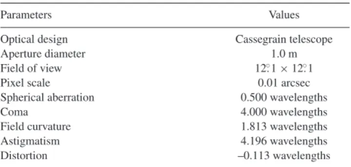
Table 1. Parameters of a simulated WFSAT for the first scenario.
Parameters Values
Optical design Cassegrain telescope
Aperture diameter 1.0 m
Field of view 12.◦1×12.◦1
Pixel scale 0.01 arcsec
Spherical aberration 0.500 wavelengths
Coma 4.000 wavelengths
Field curvature 1.813 wavelengths
Astigmatism 4.196 wavelengths
Distortion –0.113 wavelengths
3 A P P L I C AT I O N S O F T H E DA E - B A S E D P S F M O D E L
In this section, we test the performance of the DAE-based PSF modelling method with simulated data. There are three scenarios. The first is modelling the PSF for a telescope with field-dependent aberrations and the second is modelling the PSF for a telescope with static aberrations induced by atmospheric turbulence. These two scenarios are used to show that the DAE-based PSF model is capable of learning effective PSF representation, even for images with low S/N or highly variable PSFs. In the third scenario, we show that our DAE-based PSF modelling method can increase the accuracy of the secondary mirror alignment algorithm.
The DAE-based PSF model is implemented byPYTORCH (Kos-saifi et al.2019) andCUDA(Grimm & Heng2015) in a computer with Intel Core E5-2620 v3 and NVIDIA Tesla K40 GPU. Hyper-parameters, such as the learning rate, epoch size and optimization method, are important regularization conditions. In this paper, we set epoch=100, batchsize=125 and learning rate =0.00005. The Adam optimization algorithm (Kingma & Ba2014) is used for optimization with the MSE as the loss function. We discuss details of these three scenarios below.
3.1 Testing the method with a simulated WFSAT
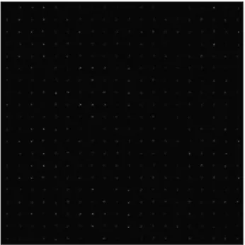
Here, we simulate a WFSAT with the parameters listed in Table1. It is a classical reflective telescope with small aberrations. However, we add large field-dependent Seidel aberrations (coma and astig-matism) to its primary mirror to increase the spatial variability of its PSFs. We calculate 121 images with size 16×16 pixels in the whole field of view through Fresnel propagation (Perrin et al.2016) and these images are separated by 1◦.1, as shown in Fig.2. Because no additional noise is added to these images, they can be viewed as PSF templates of this telescope. In this scenario, we assume that the aberrations of this telescope are known and we test whether the DAE-based PSF model can obtain PSFs from real noisy observation data. In real applications, aberrations are usually unknown to users and PSF templates obtained from real observations would be better. The data regularization condition is important for the DAE. For our application, we use two methods to generate regularized data: adding different levels of random aberrations to its primary mirror and adding different levels of noise to change the S/N of star images, as shown in Table2. The Poisson distribution is used to simulate the photon noise and the background noise. Different levels of noise are added to each data set. Note thatλ, which is shown in Table2,
denotes the worst case and it will change inside the same data set to make star images have different levels of S/N. Different levels of random wave-front aberrations, represented by low-order Zernike polynomials, are added to the primary mirror of this telescope to
PSF denoising autoencoder
655
Figure 2. The shape and position of 121 PSFs in the full field of view. Table 2. Simulated star images with different levels of noise and aberration. In Noise1,λ=0.00003, 0.00005, 0.00007 and 0.00009, respectively, in Noise2,λ=0.0003, 0.0005, 0.0007 and 0.0009, respectively, and in Noise3,
λ=0.001, 0.002, 0.003 and 0.005, respectively.λis the expectation of Poisson distribution. The 10% random aberration denotes random Seidel aberrations, which satisfies normal distribution with zero mean and variance of 10 per cent of its original aberrations. The 50% random aberration wdenotes random Zernike low-order aberrations, which satisfies normal distribution with zero mean and variance of 50 per cent of its original aberrations.
Aberration Noise1 Noise2 Noise3
10% random aberration dataset1 dataset2 dataset3 50% random aberration dataset4 dataset5 dataset6
generate random interference, which would increase the ability of the DAE to generalize. The coefficients of these random aberrations are set as a percentage of that of static Seidel coefficients. This simulation is close to real situations. During real observations, the atmospheric turbulence will introduce random aberrations and the different levels of noise will affect the S/N of observed images, while we need to obtain static aberrations represented by PSF templates from these observation data.
First, we use star images with relatively high S/N from dataset1 to train the DAE-based PSF model. We randomly pick 6724 star images as a training set and 1681 star images as a test set. After training, we use the DAE to obtain PSFs from star images in the test set. Several results are shown in Fig.3. From these figures, we can see that when the noise level is low, the DAE-based PSF model is able to obtain original PSFs from star images directly.
Then, we use star images with slightly smaller S/N to test the DAE. We also pick 6724 star images randomly as a training set and 1681 star images as a test set from dataset2. The results are shown in Fig.4. We can see that with a larger noise level, the PSF obtained by the DAE is almost the same as the original PSF. We contiguously increase the noise level and generate images with lower S/N to test the based PSF modelling method. We find that the DAE-based PSF modelling method is robust. As shown in Fig.5, when the
Figure 3. Results obtained by the DAE-based PSF model for dataset1. Images in the first row show original images, images in the second row show noisy images withσ=0.0005 and images in the third row show PSFs obtained by the DAE.
Figure 4. Results obtained by the DAE-based PSF model for dataset2. Images in the first row show original images, images in the second row show noisy images withσ=0.001 and images in the third row show PSFs obtained by the DAE.
noise level (λ) is 0.003, it is almost impossible for human beings to recognize the original PSF from star images. The DAE is still able to obtain the original PSF. We further use the structural similarity index (SSIM) and the MSE functions from the SCIKIT-IMAGEpackage (van der Walt et al. 2014) to evaluate PSFs reconstructed by the PCA-based and DAE-based PSF modelling methods. As shown in Tables3and4, the DAE-based PSF modelling method is able to
MNRAS493,651–660 (2020)
Figure 5. Results obtained by the DAE-based PSF model for dataset3. Images in the first row show original images, images in the second row show noisy images withσ=0.003 and images in the third row show PSFs obtained by the DAE.
Table 3. SSIM of dataset3.
SSIM σ=0.001 σ=0.002 σ=0.003 σ=0.005 Original noise 0.9512 0.8347 0.7326 0.5258
PCA 0.9237 0.9242 0.9220 0.9147
DAE 0.9549 0.9548 0.9544 0.9539
Table 4. MSE of dataset3.
MSE σ=0.001 σ=0.002 σ=0.003 σ=0.005 Original noise 2.6600×10⁻⁵ 1.0957×10⁻⁴ 2.1422×10⁻⁴ 6.0358×10⁻⁴ PCA 3.5375×10⁻⁵ 3.4552×10⁻⁵ 3.8546×10⁻⁵ 5.2028×10⁻⁵ DAE 2.7568×10⁻⁵ 2.7631×10⁻⁵ 2.7842×10⁻⁵ 2.8271×10⁻⁵
achieve much higher SSIM and much smaller MSE.
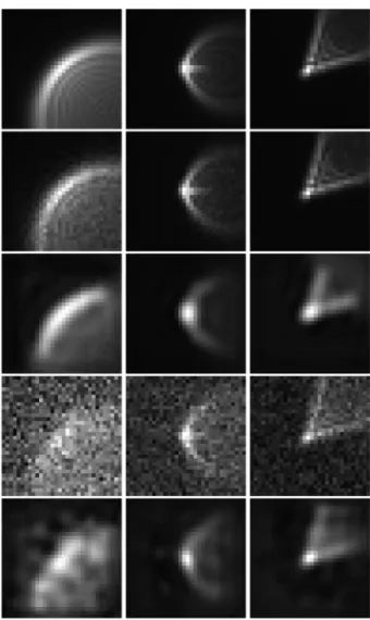
We also test the DAE-based PSF modelling method with 50 per cent random aberrations and the results are shown in Fig.6. When the S/N is large, we can see that the original PSF can be obtained. As shown in Tables5and6, we also use the SSIM and the MSE to evaluate results obtained by the DAE-based and PCA-based PSF modelling methods. We can see that the DAE-PCA-based PSF modelling method can still achieve better performance with star images of high S/N, even when the random aberration is big.
However, when we reduce the S/N, the results obtained by the DAE-based PSF modelling method are not consistent. PSFs obtained by star images at the centre of the field of view are relatively good, but PSFs obtained by star images at the edge of the field of view are not good. This is probably caused by the way we add random aberrations. As we add wave-front aberration in percentage, at the edge of the field of view, when the aberration is larger, the random interference will be larger. Large random interference will make the DAE-based PSF modelling method ineffective. Meanwhile, it also indicates that the performance of the DAE-based PSF modelling method is limited by outer interference and
Figure 6. Results obtained by the DAE-based PSF model for dataset4 and dataset5. Images in the first row show original images, images in the second row show noisy images withσ=0.00003 and images in the third row show PSFs obtained by the DAE. Images in the fourth row show noisy images withσ =0.0009, and images in the fifth row show PSFs obtained by the DAE from noisy images in the fourth row.
Table 5. SSIM of dataset5.
SSIM σ=0.0003 σ=0.0005 σ=0.0007 σ=0.0009 Original noise 0.9949 0.9853 0.9728 0.9562
PCA 0.9935 0.9937 0.9936 0.9934
DAE 0.9993 0.9993 0.9993 0.9992
Table 6. MSE of dataset5.
MSE σ=0.0003 σ=0.0005 σ=0.0007 σ=0.0009 Original noise 2.1611×10⁻⁶ 6.3513×10⁻⁶ 1.1926×10⁻⁵ 1.9634×10⁻⁵ PCA 2.5760×10⁻⁶ 2.5124×10⁻⁶ 2.6983×10⁻⁶ 2.9674×10⁻⁶ DAE 3.7504×10⁻⁷ 3.8568×10⁻⁷ 3.9869×10⁻⁷ 4.4674×10⁻⁷
random noise. When random aberration is larger than 50 per cent of its original aberrations and observed images are affected by large random noise, the DAE-based PSF modelling method cannot give promising results.
PSF denoising autoencoder
657
Figure 7. PSFs for a ideal telescope with static atmospheric turbulence aberrations. There are 400 PSFs distributed equally in a field of view of 14 arcmin.
3.2 Testing the method with a WFSAT affected by static atmospheric turbulence aberrations
Here, we consider a telescope with more complex aberrations. It is an ideal telescope with wave-front aberrations in its pupil induced by static atmospheric turbulence. In this scenario, PSFs would have highly spatial variation. We use this scenario to test the performance of the DAE in modelling complex PSFs.
We generated PSF templates with size 24 ×24 pixels in 400 locations equally distributed in a field of view of 14 arcmin, as shown in Fig.7. The atmospheric turbulence phase screen is generated by the method proposed in Jia et al. (2015a,b) and we use the Durham Adaptive Optics Simulation Platform to generate PSFs (Basden et al.2018). We add different levels of noise to the PSFs to make them as simulated star images in dataset7 and dataset8. In dataset7, Poisson noise is added to the PSFs withλ=0.0003, 0.0005, 0.0007 and 0.0009. In dataset8, Poisson noise withλ =0.001, 0.002, 0.003 and 0.005 is added to these PSFs. Theλused here is the same as we defined in Section 3.1: it stands for the worst case in each data set. We use star images from dataset7 or dataset8 to train two DAEs. We randomly pick 8000 star images as a training set and 2000 star images as a test set for each of these DAEs. After training, we use the trained DAE to obtain PSFs from star images in the test set. We find that the DAE is robust whenλ=0.0005, as shown in Fig.8. When
λ=0.005, it is almost impossible for human beings to recognize original PSFs from star images, the DAE-based PSF model can still obtain part of the original PSFs. These tests show that the DAE-based PSF modelling method has a relatively good representation ability in modelling PSFs with complex structure. However, when the S/N is extremely low, its performance will drop. We also use the SSIM and MSE to evaluate the performance of the DAE-based and PCA-based PSF modelling methods. As shown in Tables7and
8, we can see that the DAE-based PSF modelling method has better performance than the PCA-based PSF modelling method.
Figure 8. Results obtained by the DAE PSF modelling method in dataset7 and dataset8. Images in the first row are original PSFs, images in the second row show noisy images withλ=0.0005 and images in the third row show PSFs obtained by the DAE-based PSF model from noisy images in the second row. Images in the fourth row show noisy images withλ=0.005, and images in the fifth row are PSFs obtained by the DAE-based PSF model from noisy images in the fourth row.
Table 7. SSIM of dataset8.
SSIM σ=0.001 σ=0.002 σ=0.003 σ=0.005 Original noise 0.9430 0.7612 0.6866 0.4288
PCA 0.9874 0.9858 0.9832 0.9749
DAE 0.9995 0.9994 0.9994 0.9992
Table 8. MSE of dataset8.
MSE σ=0.001 σ=0.002 σ=0.003 σ=0.005 Original noise 2.6071×10⁻⁵ 1.3834×10⁻⁴ 2.0626×10⁻⁴ 6.2944×10⁻⁴ PCA 5.7382×10⁻⁶ 8.2983×10⁻⁶ 1.2569×10⁻⁵ 2.6235×10⁻⁵ DAE 7.1009×10⁻⁷ 7.6685×10⁻⁷ 8.4012×10⁻⁷ 1.0136×10⁻⁶
MNRAS493,651–660 (2020)
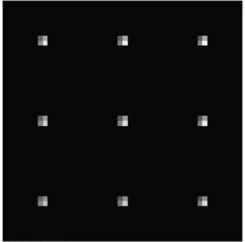
Figure 9. Distribution of star images that are used for secondary mirror alignment. They are distributed in the centre and eight corners of the field of view.
3.3 Secondary mirror alignment with a convolutional neural network and DAE PSF model
To better show increments brought by our DAE-based PSF model to other post-processing or telescope alignment methods, we con-sider a real application case in this subsection. Secondary mirror alignment is a common problem for real observations in wide-field survey telescopes, because these telescopes normally have small F-number and the performance of these telescopes is very sensitive to secondary mirror misalignment (Li, Yuan & Cui2015).
For secondary mirror alignment, astronomers need to obtain the position of the secondary mirror. We consider four degrees of freedom for the secondary mirror in this paper: decenter along theXandYdirections and tilt along theXandYdirections. Because misalignment will introduce PSF variations in the whole field of view, we can obtain the amount of misalignment according to PSFs in different field of views. Obtaining the amount of misalignment according to variation of PSFs is a traditional regression problem and it can be solved through machine learning techniques. It should be noted that we set the CCD plane in a fixed position and do not consider decenter along theZdirection, because these two degrees of freedom are highly correlated and are hard to solve directly using a machine learning algorithm.
In this paper, we consider a Ritchey–Chr´etien telescope with a field corrector, which is adapted from a sample file in Zemax. The telescope has a diameter of 1.5 m and a field of view of 1 deg. We use nine PSFs obtained from the centre and corners of the field of view to obtain the mount of misalignment, as shown in Fig.9. A simple convolutional neural network (CNN) is proposed in this paper to solve the regression problem, and the structure of this CNN is shown in Fig.10. There are five convolution layers and a fully connected layer in this CNN. We use batch normalization (Ioffe & Szegedy2015) after each convolution layer and select the Leaky–ReLU function (Laurent & von Brecht2017) as an activation function. We use the original PSFs (images with nine channels and in each channel the PSF is in a different position) as input and the
Figure 10. Structure of the CNN used for regression of secondary mirror alignment. The input dimension is 9×d×d, wheredanddare the width and height of the image, respectively. In the figure, Conv2d represents the convolutional layer and Linear represents the full connection layer. amount of misalignment (four dimensions, i.e. decenter along the xandydirections and tilt along thexandydirections) as output to train the CNN. The CNN is trained with batchsize= 10 and epoch=100. The learning rate is 0.001 at the beginning and we update the learning rate after 30 epochs with
lr=0.001∗(0.1epoch30), (14)
whereepochis the epoch number and denotes the floor function. We use the Adams algorithm with MSE loss function to update weights in the CNN. After training, the CNN can output the value of decenter and tilt along theXandYdirections directly according to nine PSFs.
The amount of misalignment lies between –0.1 to 0.1 deg for tilt and –0.1 to 0.1 cm for decenter. We obtain Zernike coefficients
PSF denoising autoencoder
659
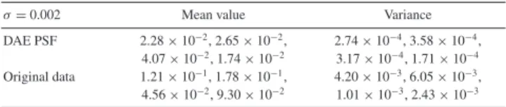
Table 9. Mean and variance of errors between the estimated and the original values of tilt and decenter for original images and PSFs obtained by the DAE PSF model with Possion noise ofλ=0.002.
σ=0.002 Mean value Variance DAE PSF 2.28×10⁻², 2.65×10⁻², 2.74×10⁻⁴, 3.58×10⁻⁴,
4.07×10⁻², 1.74×10⁻² 3.17×10⁻⁴, 1.71×10⁻⁴ Original data 1.21×10⁻¹, 1.78×10⁻¹, 4.20×10⁻³, 6.05×10⁻³, 4.56×10⁻², 9.30×10⁻² 1.01×10⁻³, 2.43×10⁻³
Table 10. Mean and variance of errors between the estimated and the original values of tilt and decenter for original images and PSFs obtained by the DAE PSF model with Possion noise ofλ=0.005.
σ=0.005 Mean value Variance DAE PSF 2.92×10⁻², 2.62×10⁻², 2.81×10⁻⁴, 3.78×10⁻⁴,
4.38×10⁻², 1.98×10⁻² 3.87×10⁻⁴, 2.07×10⁻⁴ Original data 6.76×10⁻¹, 8.02×10⁻¹, 2.36×10⁻², 3.58×10⁻², 1.39×10⁻¹, 7.32×10⁻¹ 1.62×10⁻², 1.49×10⁻²
Table 11. Correlation coefficients between estimation errors of different parameters.
Correlation coefficients decenterX–tiltY decenterY–tiltY tiltX–tiltY Original Data 0.002 0.3787 0.0937 0.1255 Original Data 0.005 0.2386 0.0128 0.1351
DAE PSF 0.002 0.1461 0.1798 0.3224
DAE PSF 0.005 0.1182 0.2098 0.3313
for different fields of view by continuously adjusting the amount of misalignment. Then we calculate PSFs according to the Zernike coefficients through Fresnel propagation (Perrin et al.2016). We obtain 625 states of misalignment and there are nine PSFs in each state. We add Poisson noise withλof 0.002 and 0.005 to these PSFs to make simulated observation images. Here,λused is the same as we defined in Sections 3.1 and 3.2 (i.e. the worst case of each data set). We use 5625 simulated PSFs to train the DAE PSF model with steps discussed at the start of Section 3. After training, the DAE PSF model can output PSFs directly according to observation images.
We generate a new set of observation images with misalignments in the same range and noise within the same level as the test set. We first input the test set into the CNN to obtain the amount of misalignment directly. The results obtained in this way stand for a common situation of secondary mirror alignment, where we directly use a trained CNN to obtain the amount of misalignment without considering the PSF model. Meanwhile, we input the test set into the DAE-based PSF model to obtain PSFs and input these PSFs into the CNN to obtain the mount of misalignment. The results are shown in Tables9and10. As can be seen from these tables, the CNN is robust to noise level, if we use it for misalignment estimation. It can give relatively good estimates regardless of the noise level. However, we also find that our DAE-based PSF model can further improve estimation accuracy when the noise level is high. These results show that our DAE PSF model can be used to increase the performance of post-processing methods.
However, it should be noted that because there are some corre-lations between tilt and decenter, the estimation accuracy of these parameters is affected by these correlations. We have calculated the correlation of errors between each predicted value, as shown in Table11. We find that decentX and tiltY, decentY and tiltY, and tiltX and tiltY have very strong positive correlations. Our DAE PSF model cannot suppress these correlations. This is a problem and we
will try to further discuss this problem in our future paper about the secondary mirror alignment method.
4 C O N C L U S I O N S A N D F U T U R E W O R K
In this paper, we propose a DAE-based PSF modelling method. Our method assumes that the PSF can be represented by the PSF templates obtained by calibration data. According to real observation conditions, we train the DAE with PSF templates and simulated observation data. After training, the DAE can be used to map any star image to its original PSF. Our method can obtain the original PSF regardless of the noise level and random aberration interference. We find that our DAE-based PSF model can increase the accuracy of the telescope’s secondary mirror alignment. Our work shows that the state of a telescope, which is represented by the PSF, can be well described by a trained neural network. It provides a new approach to understanding the PSF of telescopes. In the future, we will design post-processing methods with the DAE-based PSF model to further increase the observation data quality in WFSATs. Besides, obtaining the map between the shape of the PSF and their position in the field of view is also important. We will carry out our further research in this area in the future.
AC K N OW L E D G E M E N T S
The authors would like to thank the anonymous referee for comments and suggestions that greatly improved the quality of this manuscript. PJ would like to thank Dr Alastair Basden from Durham University and Dr Rongyu Sun from Purple Mountain Observatory, who provided very helpful suggestions for this paper. This work is supported by the National Natural Science Foundation of China (NSFC; 11503018), the Joint Research Fund in Astronomy (U1631133) under cooperative agreement between the NSFC and the Chinese Academy of Sciences (CAS),Shanxi Province Science Foundation for Youths (201901D211081), the Research and De-velopment Programme of Shanxi (201903D121161), the Research Project Supported by Shanxi Scholarship Council of China, and the Scientific and Technological Innovation Programmes of Higher Education Institutions in Shanxi (2019L0225).
R E F E R E N C E S
Bailey S., 2012,PASP, 124, 1015
Basden A. G., Bharmal N. A., Jenkins D., Morris T. J., Osborn J., Peng J., Staykov L., 2018,SoftwareX, 7, 63
Bourlard H., Kamp Y., 1988, Biological Cybernetics, 59, 291 Burd A. et al., 2005, Proc. SPIE, 5948, 59481H
Cavallari G., Ribeiro L., Ponti M., 2018, Brazilian Symposium on Computer Graphics and Image Procesing, p. 440
Cha J., Kim K. S., Lee S., 2019, preprint (arXiv:1901.08479) Grimm S. L., Heng K., 2015,ApJ, 808, 182
Hotelling H., 1933, Journal of Educational Psychology, 24, 417 Ichimura N., 2018, preprint (arXiv:1806.02336)
Ioffe S., Szegedy C., 2015, preprint (arXiv:1502.03167)
Jee M., Blakeslee J., Sirianni M., Martel A., White R., Ford H., 2007,PASP, 119, 1403
Jee M. J., Tyson J. A., 2011,PASP, 123, 596
Jia P., Cai D., Wang D., Basden A., 2015a,MNRAS, 447, 3467 Jia P., Cai D., Wang D., Basden A., 2015b,MNRAS, 450, 38 Jia P., Sun R., Wang W., Cai D., Liu H., 2017,MNRAS, 470, 1950 Kingma D. P., Ba J., 2014, preprint (arXiv:1412.6980)
Kohonen T., 1982, Biological Cybernetics, 43, 59
Kossaifi J., Panagakis Y., Anandkumar A., Pantic M., 2019, J. Mach. Learn Res., 20, 925
MNRAS493,651–660 (2020)
Laurent T., von Brecht J., 2017, preprint (arXiv:1712.10132) Li Z., Yuan X., Cui X., 2015,MNRAS, 449, 425
Li B.-S., Li G.-L., Cheng J., Peterson J., Cui W., 2016, Res. Astron. Astrophys., 16, 139
Ma Y., Zhao H., Yao D., 2007, in Valsecchi G. B., Vokrouhlick´y D., Milani A., eds, Proc. IAU Symp. Vol. 236, Near Earth Objects, Our Celestial Neighbors: Opportunity and Risk. Kluwer, Dordrecht, p. 381 Makidon R., Casertano S., Cox C., van der Marel R., 2007, NASA Technic
Al Report, 23, 155 Moffat A., 1969, A&A, 3, 455
Perrin M., Long J., Douglas E., Sivaramakrishnan A., Slocum C., 2016, POPPY: Physical Optics Propagation in PYthon, (ascl:1602.018) Perrin M. D., Sivaramakrishnan A., Lajoie C., Elliott E., Pueyo L.,
Ravin-dranath S., Albert L., 2014, Proc. SPIE, 9143, 91433X Ping Y., Zhang C., 2017,Adv. Space Res., 60, 907 Piotrowski L. W. et al., 2013, A&A, 551, A119 Racine R., 1996,PASP, 108, 699
Ratzloff J. K., Law N. M., Fors O., Corbett H. T., Howard W. S., Ser D. D., Haislip J. B., 2019,PASP, 131, 075001
Rhodes J., Massey R., Albert J., Taylor J. E., Koekemoer A. M., Leauthaud A., 2005, preprint (arxiv:0512.170)
Rhodes J. D. et al., 2007,ApJS, 172, 203 Sun R., Jia P., 2017,PASP, 129, 044502 Sun R., Yu S., 2019,Ap&SS, 364, 39 van der Walt S. et al., 2014, PeerJ, 2, e453
Vidal R., Ma Y., Sastry S. S., 2005, IEEE Transactions on Pattern Analysis and Machine Intelligence, 27, 1945
Vincent P., Larochelle H., Bengio Y., Manzagol P.-A., 2008, Proceedings of the 25th International Conference on Macline Learning, p. 1096 Vincent P., Larochelle H., Lajoie I., Bengio Y., Manzagol P.-A., 2010, J.
Mach. Learn Res., 11, 3371
Wang W., Jia P., Cai D., Liu H., 2018,MNRAS, 478, 5671
This paper has been typeset from a TEX/LATEX file prepared by the author.