S.A. Alumur I B.Y. Kara I M.T. Melo
Location and Logistics
Schriftenreihe Logistik der Fakultät für Wirtschaftswissenschaften
der htw saar
Technical reports on Logistics of the Saarland Business School
Nr. 5 (2013)
© 2013 by Hochschule für Technik und Wirtschaft des Saarlandes, Fakultät für Wirtschaftswissenschaften, Saarland Business School
ISSN 2193-7761
Location and Logistics
S.A. Alumur I B.Y. Kara I M.T. Melo Bericht/Technical Report 5 (2013)
Verantwortlich für den Inhalt der Beiträge sind die jeweils genannten Autoren.
Alle Rechte vorbehalten. Ohne ausdrückliche schriftliche Genehmigung des Herausgebers darf der Bericht oder Teile davon nicht in irgendeiner Form – durch Fotokopie, Mikrofilm oder andere Verfahren - reproduziert werden. Die Rechte der öffentlichen Wie-dergabe durch Vortrag oder ähnliche Wege bleiben ebenfalls vorbehalten.
Die Veröffentlichungen in der Berichtsreihe der Fakultät für Wirtschaftswissenschaften können bezogen werden über: Hochschule für Technik und Wirtschaft des Saarlandes
Fakultät für Wirtschaftswissenschaften Campus Rotenbühl
Waldhausweg 14 D-66123 Saarbrücken
Location and Logistics
∗
Sibel A. Alumur
a, Bahar Y. Kara
b, M. Teresa Melo
c,d aDepartment of Industrial Engineering, TOBB University of Economics and Technology, Ankara, Turkey
b
Department of Industrial Engineering, Bilkent University, Ankara, Turkey
c
Business School, Saarland University of Applied Sciences, Saarbr¨ucken, Germany
d
Operations Research Center, Faculty of Sciences, University of Lisbon, Lisbon, Portugal
Abstract
Facility location decisions play a critical role in designing logistics networks. This article provides some guidelines on how location decisions and logistics functions can be integrated into a single mathematical model to optimize the configuration of a logistics network. This will be illustrated by two generic models, one supporting the design of a forward logistics network and the other addressing the specific requirements of a reverse logistics network. Several special cases and extensions of the two models are discussed and their relation with the scientific literature is described. In addition, some interesting applications are outlined that demonstrate the interaction of location and logistics de-cisions. Finally, new research directions and emerging trends in logistics network design are provided.
Keywords: forward logistics network design, reverse logistics network design, models, applications.
1
Introduction
Logistics network design (LND) and facility location decisions are closely interrelated. The latter are prompted by the need either to build a new logistics network or to re-design a network that is already in place. When a company enters new markets or grows into new product segments, a new logistics network has to be designed. However, “green field” projects are less frequent compared with re-design initiatives. Changing market and business conditions compel a company to modify the physical structure of its logistics network from time to time. Major drivers of network re-design projects comprise variations in the demand pattern and its spatial
∗This article will appear in Location Science, G. Laporte, S. Nickel, F. Saldanha-da-Gama, editors,
distribution as well as increased cost pressure and service requirements. Moreover, mergers, acquisitions, and strategic alliances also trigger the expansion or reconfiguration of a logistics network in order to exploit the benefits and synergies of integrating the acquired operations. Typically, re-design activities take the form of opening new facilities (e.g. to be closer to new markets) and closing existing facilities (e.g. to consolidate operations). As highlighted by Ballou (2001) and Harrison (2004), well-conceived re-design decisions can result in a 5 to 15 percent reduction of the overall logistics costs, with 10 percent being often achieved.
The (re-)design of a logistics network is a complex undertaking. It concerns not only determining the number, size, and capacity of facilities (e.g. plants, warehouses) to be operated but it also involves planning and integrating a manifold of logistics functions that such facilities will perform. These functions range from procurement of raw materials, transformation of these materials into semi-finished and end products, and the delivery of finished products to customers through one or several distribution stages. Depending on the industrial context, strategic decisions may also concern the collection and recovery of product returns.
This article provides a holistic approach to strategic network planning by integrating facility location decisions with other decisions relevant to the configuration of a logistics network. This will be illustrated by two general mathematical modeling frameworks for designing forward and reverse logistics networks.
The remainder of the article is organized as follows. Section 2 presents a comprehensive model for logistics networks with forward flows. Due to its generic features, the model applies to a wide range of situations. Its relation with other models proposed in the literature is established and extensions are discussed. Section 3 focuses on reverse logistics network design (RLND) and introduces a generic mathematical formulation for the design of a multi-purpose reverse logistics network. Furthermore, some special cases and extensions of the proposed model are presented. Section 4 addresses various representative applications of forward and reverse LND problems from different areas. Finally, in Section 5 future research directions are discussed.
2
A General Logistics Network Design Model
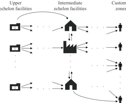
We introduce a base model that captures the main features of an LND problem. The starting point is either a potential framework for a new network structure or an existing network whose physical structure is to be re-designed. To this end, a general network typology, as depicted in Figure 1, is considered. Any number of facility layers and any system of transportation
channels can be modeled. The network entities are categorized in so-calledselectable and non-selectable facilities. The former group includes a set of facilities already in place, that could be closed, and a set of potential locations for establishing new facilities. In contrast, non-selectable facilities comprise facilities that are not subject to location decisions. Typically, such facilities include suppliers as well as existing plants and/or warehouses that must be maintained. In addition, customer zones are viewed as special members of this set as they have demand requirements for multiple commodities. As shown in Figure 1, no restrictions are imposed on the availability of transportation channels for the flow of materials through the network. In particular, direct commodity flows from upstream sources to customer zones (or to facilities not immediately below in the hierarchy) are possible as well as flows between facilities in the same echelon. In this rather general network typology, procurement, production, distribution, and customer service decisions are to be made along with facility location and sizing decisions. The mathematical model in Section 2.2 captures the aforementioned features. The required notation is first introduced in Section 2.1. Several special cases and extensions are discussed in Section 2.3. Customer zones Upper echelon facilities Intermediate echelon facilities . . . . . . . . . . . . . . . . . . . . . . . . . . . . . .
2.1
Notation and Definition of Decision Variables
Table 1 introduces the index sets that are used in the base model. In addition to the various types of network entities, also multiple commodities are considered, ranging from raw materials and intermediate products to finished goods. Moreover, different kinds of resources may be available for manufacturing and handling commodities.
Symbol Description
In Set of potential locations for new facilities
Ie Set of existing facilities that could be closed
I Set of selectable facilities, I =Ie∪In
J Set of non-selectable locations (e.g. customer zones)
L Set of all entities, L=I∪J
P Set of products
Rm, Rh Set of manufacturing / handling resources
Table 1: Index sets
Table 2 describes input parameters related to logistics operations. Multi-stage production processes can be taken into account through bills-of-materials (BOMs). In this case, the relationships between components and parent items are defined by given parameters. Capacities of service facilities are modeled in a general way through production and handling resources. Three different types of association are considered. In a many-to-one relationship, several
Symbol Description
dℓp Demand of location ℓ ∈ L for product p ∈ P (typically, dℓp = 0 for
ℓ ∈I)
αℓqp Number of units of product q ∈ P required to manufacture one unit
of product p∈P (q 6=p) at facility ℓ ∈L
µℓrp Number of units of resource r∈Rm required to manufacture one unit
of product p∈P at facility ℓ∈L λi
ℓrp, λoℓrp Number of units of resource r ∈ Rh required to handle one unit of
product p∈P upon its arrival at / shipment out of facility ℓ ∈L Km
r , Krh Capacity of production / handling resource r∈Rm/Rh
EKm
r , EKrh Maximum increase in capacity of production / handling resource
r ∈Rm/Rh
resources are available at the same facility. Some resources may be product-specific (e.g. a machine dedicated to a given item) while others may be shared by multiple commodities (e.g. a production line or order picking system). Aone-to-one association corresponds to the classical way of modeling capacity in facility location models (e.g. storage space in a warehouse). One-to-many relationships can also be modeled, although these are less common. This could be the case, for example, of a team of experts responsible for several production lines in different facilities. Resource availability can be increased at additional expense, e.g. through overtime work or leasing extra storage space. Resource consumption is described by specific parameters. In the case of handling resources, the same type of equipment (e.g. a forklift truck) may be required with different intensity to unload incoming goods at a facility and load goods to be shipped out of the same facility.
Table 3 summarizes all facility and logistics costs. Facility costs are related to establishing new facilities and closing existing facilities, and typically reflect economies of scale. In addi-tion, facility operating costs represent, for example, business overhead costs such as staff and security costs. Logistics costs are incurred for purchasing items from external sources (e.g. procurement of raw materials), for manufacturing commodities, and for distributing multiple products through the network. The latter costs may also include charges for handling goods at the source facility and at the destination facility (e.g. order picking and warehousing costs). Furthermore, additional costs are considered for resource expansion. Penalty costs are also incurred for failing to meet customer demand. These costs represent the additional expense for
Symbol Description
F Cℓ Fixed setup cost of establishing a new facility in location ℓ ∈In
SCℓ Fixed cost of closing existing facility ℓ ∈Ie
OCℓ Fixed cost of operating facility ℓ∈L
P Cℓp Unit cost of purchasing product p ∈ P at facility ℓ ∈ L from an
external source
MCℓp Unit cost of manufacturing product p∈P at facility ℓ∈L
T Cℓℓ′p Unit cost of transporting product p∈P from facility ℓ∈Lto facility
ℓ′ ∈L (ℓ 6=ℓ′)
ECm
r , ECrh Unit cost of expanding production / handling resource r∈Rm/Rh
DCℓp Unit penalty cost for not serving demand of facility ℓ∈Lfor product
p∈P
outsourcing unfilled demand.
Finally, strategic decisions on facility location and logistics operations are ruled by the variables in Table 4.
Symbol Description
yℓ 1 if the selectable facility ℓ∈I is operated, 0 otherwise
sℓp Quantity of product p ∈P purchased at facility ℓ ∈L from an external
source
zℓp Quantity of product p∈P manufactured at facilityℓ ∈L
xℓℓ′p Quantity of product p ∈P shipped from facility ℓ ∈L to facility ℓ′ ∈ L (ℓ6=ℓ′)
wm
r , wrh Number of extra capacity units of production / handling resource r ∈
Rm/Rh
uℓp Quantity of unsatisfied demand of location ℓ∈L for product p∈P
Table 4: Decision variables
2.2
A Mixed-Integer Linear Programming Model
Under the assumption that all inputs are known nonnegative quantities, the logistics network (re-)design problem can be formulated as a mixed-integer linear program (MILP) as follows.
The objective function (1) describes the aim of the decision-making process, namely to identify the network configuration with the least total cost. To this end, fixed costs associated with opening, closing, and operating facilities are considered. Variable costs account for resource expansion and for material procurement, production and distribution. In addition, penalty costs are incurred to unfilled demand.
(P1) MIN X ℓ∈In F Cℓyℓ + X ℓ∈Ie SCℓ(1−yℓ) + X ℓ∈I OCℓyℓ + X ℓ∈J OCℓ+ X r∈Rm ECrmw m r + X r∈Rh ECrhw h r + X ℓ∈L X p∈P P Cℓpsℓp+ X ℓ∈L X p∈P MCℓpzℓp + X ℓ∈L X ℓ′∈L\{ℓ} X p∈P T Cℓℓ′pxℓℓ′p + X ℓ∈L X p∈P DCℓpuℓp (1)
s.t. sℓp+ X ℓ′∈L\{ℓ} xℓ′ℓp+zℓp = X q∈P αℓpqzℓq+ X ℓ′∈L\{ℓ} xℓℓ′p+dℓp−uℓp ℓ ∈L, p∈P (2) X ℓ∈L X p∈P µℓrpzℓp ≤Krm+w m r r ∈R m (3) X ℓ∈L X p∈P λi ℓrpsℓp+ X ℓ∈L X ℓ′∈L\{ℓ} X p∈P λo ℓrp+ λiℓ′rp xℓℓ′p ≤Krh+whr r ∈Rh (4) 0≤wm r ≤EK m r r ∈R m (5) 0≤wrh ≤EK h r r ∈R h (6) 0≤uℓp≤dℓp ℓ ∈L, p∈P (7) 0≤sℓp ≤M yℓ, 0≤zℓp≤M yℓ ℓ ∈I, p∈P (8) 0≤xℓℓ′p ≤M yℓ ℓ ∈I, ℓ′ ∈L\ {ℓ}, p∈P (9) 0≤xℓℓ′p ≤M yℓ′ ℓ ∈L\ {ℓ′}, ℓ′ ∈I, p∈P (10) sℓp≥0, zℓp ≥0, xℓℓ′p ≥0 ℓ, ℓ′ ∈J (ℓ 6=ℓ′), p∈P (11) yℓ ∈ {0,1} ℓ ∈I (12)
Constraints (2) are the usual flow balance equations. The inbound flow of an item to a facility consists of procuring or producing the item at the facility or receiving it from other locations. The outbound flow results from using the product as a raw material to manufacture other commodities, distributing the item to other facilities, or serving demand in case the lo-cation is a customer zone. Inequalities (3), resp. (4), guarantee that the usage of production, resp. handling, resources does not exceed the available capacity. Constraints (5)–(6) stipu-late that capacity expansions must be within given limits. Constraints (7) rule the maximum amount of unsatisfied demand. Inequalities (8)–(10) ensure that procurement, production, and distribution activities only occur at operating facilities. A sufficiently large constant M is used in these constraints which can be adjusted depending on each specific situation. Typically, M
is replaced by the maximum quantity that can be processed by a facility with respect to all product types.
non-selectable locations, while constraints (12) are binary requirements for the location variables. Although the above problem is NP-hard, being a generalization of the simple plant location problem (see Krarup and Pruzan (1983)), Melo et al. (2008) could solve medium and large-sized randomly generated instances to optimality with a general purpose optimization software within reasonable time. To analyze the quality of the MILP formulation, the linear relaxation bound was also compared with the optimal solution of the tested instances. In general, a relatively small gap could be observed. These findings have important practical implications, since managers often need to base their decisions on the results of several scenarios. Hence, for a company to be able to perform “what-if” analyzes and thereby identify good quality (or even optimal) solutions with an acceptable level of computational effort is a major step towards better decision support.
2.3
Special Cases and Model Extensions
Historically, researchers have focused relatively early on the design of distribution systems with at most two facility layers (e.g. plants, warehouses). In these simple networks, decisions were mostly confined to facility location and distribution operations. The contribution by Geoffrion and Graves (1974) is such an example. In recent years, the trend has been towards the devel-opment of more comprehensive models that integrate location decisions with supplier selection, production planning, technology acquisition, inventory management, transportation mode selec-tion, and vehicle routing, just to mention some important logistics functions considered in this area (see Melo et al. (2009) for a comprehensive review). In many cases, the proposed models combine strategic decisions (e.g. location and capacity choices) with tactical decisions (e.g. inventory and transportation management) or even operational decisions (e.g. vehicle routing). Usually, the interplay of different planning levels can only be captured at the cost of increased model complexity. This will be illustrated in Section 4 by three applications.
The generic formulation(P1)comprises some of the aforementioned features and it can also
be adapted or extended to include further aspects relevant to LND. For example, it is easy to add single-sourcing requirements to(P1)to ensure that the demand of each customer zone for a particular product is entirely satisfied from a unique facility. A straightforward extension of(P1)
is also to embed the (re-)design of a logistics network in a multi-period planning horizon. Such a setting is meaningful since the establishment of new facilities is typically a long-term project involving time-consuming activities and requiring substantial investment capital. In this case,
strategic decisions can be constrained by the budget available in each time period. Logistics decisions will be in turn impacted by the location choices. Fleischmann et al. (2006) and more recently Correia et al. (2013) included this feature in their dynamic network design models.
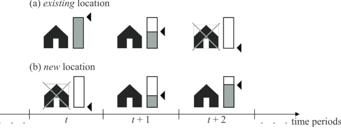
A multi-period setting is also appropriate for planning the re-design of a logistics network that is already in place. In this context, existing facilities may have their capacities expanded, reduced or even moved to new sites over several time periods as illustrated in Figure 2 (the bars in the figure next to the facilities indicate their size). In turn, new facilities can be established through successive sizing. A gradual transfer of production and/or storage capacities from existing locations to new sites ensures a smooth implementation of relocation plans and avoids logistics operations from being disrupted. Melo et al. (2006, 2011, 2012) proposed several models and heuristics for this special form of network re-design.
(a)existinglocation
time periods t t+ 1 t+ 2 . . . (b)newlocation . . .
Figure 2: Facility sizing over multiple periods (the crossed symbol indicates a closed facility)
Finally, the growth in globalization has led to the emergence of global supply chains, that is, worldwide networks of suppliers, manufacturers, distribution centers, and retailers. Con-sequently, the integration of financial considerations with location and logistics decisions has gained increasing importance in network design. Financial factors comprise, among others, taxes, duties, tariffs, exchange rates, and transfer prices. Meixell and Gargeya (2005) discuss various contributions in this area while Wilhelm et al. (2005) propose a comprehensive model for the design of a logistics network under the North American Free Trade Agreement (NAFTA).
3
A General Reverse Logistics Network Design Model
Reverse logistics refers to all operations involved in the return of products and materials from a point of use to a point of recovery or proper disposal. The purpose of recovery is to recapture value through options such as reusing, repairing, refurbishing, remanufacturing, and recycling. Reverse logistics includes the management of the return of end-of-use or end-of-life products as well as defective and damaged items, or packaging materials, containers, and pallets.
Major driving forces behind reverse logistics activities include economical factors, legislations, and environmental consciousness. As stated by De Brito and Dekker (2004) companies become active in reverse logistics because they can make a profit and/or because they are forced to focus on such functions, and/or because they feel socially motivated. These factors are usually intertwined. For example, a company can be compelled to reuse a certain percentage of components in order to achieve a recovery target set by the legislation. This will lead to a decrease in the cost of purchasing components and in waste generation. Jayaraman and Luo (2007) suggest that proper management of reverse logistics operations can lead to greater profitability and customer satisfaction, and at the same time be beneficial for the environment. Many actors are involved in the design and operation of a reverse logistics network. Even though extended producer responsibilities present in the legislations in various countries give the responsibility of recovering used products to original equipment manufacturers, governments need to establish the necessary infrastructure. Responsibilities can be shared among different parties, such as producers, distributors, third-party logistics providers, or municipalities, in designing and operating the reverse logistics networks.
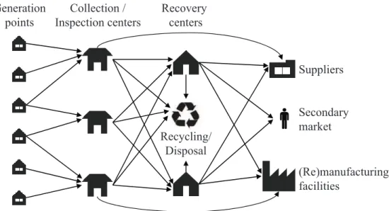
In a reverse logistics network, the end-of-life or end-of-use products can be generated at private households and at commercial, industrial, and institutional sources, which are referred to as generation points. Products are usually collected at special storage facilities called collection or inspection centers. Products are then sent for proper recovery through reusing, repairing, refurbishing, remanufacturing, or recycling. Inspected or recovered products and components can then be sold to suppliers, to (re)manufacturing facilities, or to customers in secondary markets. A generic reverse logistics network is depicted in Figure 3.
Unlike forward logistics networks, where demand occurs at the lower echelon facilities, in reverse networks demand (for recovery) arises at the upper echelon facilities. However, a reverse logistics network is not a mirror image of a forward network. In addition to the typical forward supply chain actors, different actors and facilities are involved in reverse logistics
Recycling/ Disposal Collection / Inspection centers Suppliers Secondary market (Re)manufacturing facilities Recovery centers Generation points
Figure 3: A generic reverse logistics network
networks, such as disposers, remanufacturers, and secondary markets. Moreover, unlike forward networks, which are mostly driven by economical factors, there are further factors motivating the establishment of reverse logistics networks such as environmental laws.
In Section 3.2, a generic mathematical formulation for the design of a multi-purpose reverse logistics network is presented. The required notation and the decision variables are first defined in the next section. Section 3.3 discusses some special cases and possible extensions of the proposed model.
3.1
Notation and Definition of Decision Variables
The notation used in the generic RLND model is analogous to the notation introduced in Section 2.1 for the forward LND model. Similar to the forward network design problem, multiple commodities are considered in the configuration of the reverse logistics network. These are represented by the setP, which may include used, inspected, repaired, or refurbished products, components, or raw materials. In order to represent a different state (inspected, repaired, refurbished, etc.) of a certain type of product, a different product type needs to be defined within the set P. Table 5 describes all index sets that are required for modeling the RLND problem.
re-Symbol Description
R Set of recovery options (e.g. repair, refurbish, recycle)
Irn Set of potential locations for recovery option r∈R
Ire Set of existing facilities with recovery option r∈R
Ir Set of selectable facilities with recovery option r ∈R, Ir =Irn∪Ire
Jr Set of non-selectable locations with recovery optionr∈R(e.g. secondary
market, disposal)
L Set of all locations, L=Ir∪Jr
Table 5: New index sets
furbish, and recycle as well as other options such as inspection, disassembly, selling to suppliers, to secondary markets or to external (re)manufacturing facilities, and disposal. Even though the latter options may not be regarded as recovery alternatives, in order to provide a generic model incorporating all the decisions present in real-life reverse logistics networks, they are included in the set R. Observe that some recovery options may be operated by third-party logistics providers. These external facilities also belong to the set Jr. Moreover, it is assumed that
generation points are also included in this set of non-selectable facilities.
Table 6 introduces the required parameters. Transitions between the stages of products and reverse BOMs are taken into account through the β parameter. For example, a damaged product can be converted into a repaired product through the recovery option repair, or a used product can be disassembled into its components at a disassembly facility. Each recovery option has a given capacity which can be expanded at selectable facilities. Revenues may be obtained through some recovery options, e.g. by selling products or components to recycling facilities, to secondary markets or to external (re)manufacturing facilities. Some recovery options may also incur costs as in the case of product disposal.
Finally, Table 7 describes the decision variables. The RNLD model also uses the flow variables x introduced in Table 4.
3.2
A Mixed-Integer Linear Programming Model
With the notation defined in the previous section, the reverse logistics network (re-)design problem can be formulated as an MILP as follows. The objective function (13) maximizes the total profit. It sums the revenues obtained from various recovery options (e.g. by sending products to recycling facilities, by selling products to secondary markets) and subtracts the
Symbol Description
gℓp Amount of product p∈P generated at location ℓ∈L
βrqp Number of units of product p ∈ P obtained by processing one unit of
product q∈P (q6=p) using recovery option r∈R Krℓ Capacity of recovery option r∈R at location ℓ∈L
EKrℓ Maximum increase in capacity for recovery option r ∈ R at location
ℓ∈Ir
RTrp Recovery target for product p∈P with recovery option r∈R
RErℓp Revenue from recovering one unit of productp∈P with recovery option
r∈Rat locationℓ∈L(e.g. revenue from recycling or from the secondary market)
RCrℓp Cost of recovering one unit of productp∈P with recovery option r∈R
at location ℓ ∈L
F Crℓ Fixed setup cost of establishing recovery optionr ∈Rin locationℓ∈Irn
SCrℓ Fixed cost of closing recovery option r∈R at existing facility ℓ∈Ire
OCrℓ Fixed cost of operating recovery option r∈R at location ℓ∈L
ECrℓ Unit cost of expanding capacity of recovery option r ∈ R at location
ℓ∈Ir
Table 6: New parameters
Symbol Description
yrℓ 1 if recovery option r∈ R is operated at the selectable facility ℓ ∈Ir, 0
otherwise
vrℓp Amount of product p ∈ P recovered with recovery option r ∈ R at
location ℓ∈L
wrℓ Number of extra capacity units established for recovery option r ∈R at
location ℓ∈Ir
Table 7: New decision variables
total cost of establishing and operating the network. The latter comprises the cost of recovering products at facilities, of setting up new recovery options at facilities, of closing existing recovery options, of operating new and existing recovery options at facilities, of transporting products, and of expanding the capacities of recovery options.
(P2) MAX X r∈R X ℓ∈L X p∈P RErℓpvrℓp− X r∈R X ℓ∈L X p∈P RCrℓpvrℓp− X r∈R X ℓ∈Irn F Crℓyrℓ
−X r∈R X ℓ∈Ire SCrℓ(1−yrℓ)− X r∈R X ℓ∈Ir OCrℓyrℓ− X r∈R X ℓ∈Jr OCrℓ −X ℓ∈L X ℓ′∈L\{ℓ} X p∈P T Cℓℓ′pxℓℓ′p− X r∈R X ℓ∈Ir ECrℓwrℓ (13) s.t. gℓp+ X r∈R X q∈P βrqpvrℓq+ X ℓ′∈L\{ℓ} xℓ′ℓp= X r∈R vrℓp+ X ℓ′∈L\{ℓ} xℓℓ′p ℓ∈L, p∈P (14) X ℓ∈L vrℓp≥RTrp r ∈R, p ∈P (15) X p∈P vrℓp≤Krℓyrℓ+wrℓ r ∈R, ℓ∈Ir (16) X p∈P vrℓp≤Krℓ r ∈R, ℓ∈Jr (17) 0≤wrℓ ≤EKrℓyrℓ r ∈R, ℓ∈Ir (18) 0≤xℓℓ′p ≤M X r∈R yrℓ ℓ∈Ir, ℓ′ ∈L\ {ℓ}, p∈P (19) 0≤xℓℓ′p ≤M X r∈R yrℓ′ ℓ∈L\ {ℓ′}, ℓ′ ∈Ir, p∈P (20) xℓℓ′p ≥0 ℓ, ℓ′ ∈Jr(ℓ6=ℓ′), p∈P (21) vrℓp≥0 r ∈R, ℓ∈L, p∈P (22) yrℓ ∈ {0,1} r ∈R, ℓ∈Ir (23)
Equalities (14) are the flow balance constraints. For each location and product, the total inflow comprises the amount of product generated at that location, the total amount of product arising after processing various items, and the total amount of product shipped to this location from other locations. The total inflow is equal to the total outflow which includes the total amount of product recovered at that location and the total amount of product shipped to other locations. Constraints (15) ensure that the recovery target for each product category and recovery option is met. Recovery targets are usually stipulated by legislations for different types of recovery options. Inequalities (16)–(18) are the capacity constraints. Constraints (16) guarantee that the total amount of recovered products at the selectable facilities does not exceed the total capacity. Similar conditions are set at non-selectable facilities by inequalities (17). Constraints (18) restrict the expansion of capacity at selectable facilities to be within given
limits. Similar to the forward LND model, constraints (19)–(20) impose that products can only be shipped from operated facilities. Lastly, conditions (21)–(23) set the domains of the decision variables.
The proposed model is generic in the sense that it includes multiple types of products and components at different stages (inspected, repaired, refurbished, etc.). Moreover, it considers reverse BOMs and transitions between the stages of products through various recovery options. Along with conventional recovery options, such as repair, refurbish, and recycle, it is also possible to include further options such as inspection, disassembly, selling to external facilities, and disposal. The problem is modeled with a profit oriented objective function accounting for the revenues from different recovery options in addition to costs.
In terms of problem complexity, the above RLND model has similar attributes to the forward network design problem (P1). Moreover, general purpose optimization software (e.g. CPLEX,
Gurobi) can be used to solve (P2). However, for large-sized instances there may be a need for
customized algorithms and heuristics.
3.3
Special Cases and Model Extensions
The generic model (P2) can be easily tailored to different applications. A reverse logistics network design application for the collection and recovery of waste electrical and electronic equipment is detailed in Section 4.4.
The term closed-loop supply chain refers to a network comprising both forward and reverse flows. Figure 4 depicts the structure of such a network. The cost of processing a return flow in a supply chain designed by considering only forward flows can be much higher than processing a flow in the forward direction. Thus, supply chain networks that include flows in the reverse direction should be designed by integrating forward and reverse logistics activities. The models introduced in Sections 2.2 and 3.2 are readily extendible to the design of closed-loop supply chains. The interested reader is referred to Krikke et al. (2003), Easwaran and ¨Uster (2009), and Salema et al. (2010) for exemplary studies determining the locations of facilities within closed-loop supply chain networks.
As emphasized in Section 2.3, the dynamic nature of the (re-)design problem should not be disregarded. Multi-period models in RLND were proposed, for example, by Lee and Dong (2009), Salema et al. (2010), and Alumur et al. (2012).
Suppliers Production Consumers facilities Distribution centers Remanufacturing facilities Recycling / Disposal
Forward flows Reverse flows
Collection / Inspection / Recovery centers
Figure 4: A closed-loop supply chain network
arise at the upper echelon facilities (e.g. uncertainty in the amount and in the quality of returned products). There are some studies addressing uncertainty issues within the context of RLND such as Realff et al. (2004), Liste¸s and Dekker (2005), Salema et al. (2007), and Fonseca et al. (2010).
As discussed at the beginning of Section 3, major driving forces in reverse logistics networks include not only economical factors, but also legislations and environmental consciousness. Thus, in addition to the actors involved in forward logistics networks, also actors such as mu-nicipalities, foundations, third-party logistics providers, and disposers, are involved in designing and operating reverse logistics networks. Multiple actors lead to decision problems with multiple objectives. Even though there are some studies that consider the multi-objective nature of this design problem (e.g. Pati et al. (2008), Fonseca et al. (2010), Basmacı and Alumur (2014)), this issue requires further attention.
For other extensions and special cases on RLND, the interested reader is referred to the reviews by Fleischmann et al. (2004), Bostel et al. (2005), Ak¸calı et al. (2009), and Aras et al. (2010).
4
Applications
The aim of this section is to demonstrate the richness in LND through presenting applications from various areas including organ transportation in addition to more classical areas. The general form of the models described in Sections 2 and 3 allows them to be applied to an LND problem of a manufacturer as well as of a logistics service provider under appropriate set, parameter, and variable definitions.
In this section, four applications from different sectors are discussed. Section 4.1 presents the network design problem of a global beverage company. Many companies utilize logistics service providers, namely third-party logistics companies, in their distribution networks. In Section 4.2 an application from this area is provided. Section 4.3 is devoted to an atypical application in LND arising in organ transportation. The problem has additional features resulting from the nature of the good being transported. Finally, Section 4.4 illustrates an application for waste electrical and electronic equipment.
4.1
Logistics Network Design of a Beverage Company
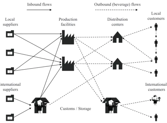
Beverage companies usually operate bottling factories in which the required materials are mixed, bottled, and then packaged to be shipped to end users. Global companies usually need to import some of the input materials, like flavors and syrups, to guarantee the same quality worldwide. Moreover, ingredients may also be provided by local suppliers. Thus, inbound logistics involves both international and national shipments to the manufacturing plant. In turn, the outbound flow from the plant comprises bottled and packaged beverages ready to consume. The flow of end products may also be targeted at neighboring countries, thus involving again national and international shipping. The schematic representation of the logistics network, which is a specialized version of Figure 1, is given in Figure 5.
The main decisions in this LND problem include the location of new distribution centers (DCs) and the choice of transportation channels for the inbound and outbound flows of these DCs. As can be seen from Figure 5, the manufacturer may choose to operate additional DCs closer to the customs area to ease the overall customs process. Certain beverages are not produced in every country. Thus, there is a bottled beverage flow from the customs area towards DCs for those products that are not manufactured in a country. Shipments to international customers (via the customs) consist mainly of products that are produced in the local country and they will constitute the in-country product flow in the LND problems of other countries.
Local suppliers Local customers Production facilities Distribution centers
Inbound flows Outbound (beverage) flows
International suppliers
Customs / Storage
International customers
Figure 5: Logistics network of a beverage company
Observe here that, in addition to finding the locations of DCs and deciding on the trans-portation structures to use, the LND problem also includes routing decisions for deliveries to the customers (see the dashed lines in Figure 5). Typically, a global beverage company resorts to third-party logistics service providers to handle the distribution of orders to end users. The service provider operates its own logistics network, which will be detailed in the next subsection. Apart from location and routing decisions, a typical beverage company also questions:
• the level of inventories at the DCs,
• the need for consolidation; some examples include consolidation on the route and consol-idation at the facility,
• the transportation mode to be utilized (especially between plants and warehouses rail transportation is a valid option).
A beverage company is also engaged in reverse logistics activities through the return of empty flagons to the manufacturing plant. Typically, a third-party service provider combines the delivery of beverages to customers with the collection of empty refillable beverage containers.
4.2
Logistics Network Design of a Third-Party Logistics
Com-pany
LND is a crucial problem for Third-Party Logistics (3PL) companies since they offer warehousing and transportation services to multiple manufacturers having specific requirements. A typical 3PL company generally operates based on yearly contracts, each defining the level of integration to be provided to the customer. This can range from basic services, which mainly handle the transportation aspect of the overall distribution network, to integrated logistics activities, which can even include packaging, labeling, and customs clearance type of services. The design of the network of a 3PL company is, of course, influenced by the level of integration. Nevertheless, a typical 3PL provider usually operates several DCs and the number of DCs is based on the geographical span and on the promised service levels. Since the logistics network of a 3PL company does not include inbound shipments towards production plants, a generic network is composed of production facilities, DCs, and customers (cf. Figure 1). The main decisions to be made in the LND problem include the location of DCs and the choice of appropriate transportation structures.
Consolidation is a crucial aspect in the distribution network of a 3PL company. Especially in small geographical regions, say in urban areas, companies try to consolidate customer orders into full truckload shipments. As a result, delivery and/or collection vehicles serve many customers on each route they travel.
Typically, a 3PL company operates a few DCs and delivery vehicles travel from/to DCs to service customers. In the upper echelon of the network products flow from factories or central warehouses to DCs. Thus, a 3PL company may consolidate shipments in both stages of the network. Different modes of transportation may be used for bulk transportation from upper echelon facilities.
By nature, 3PL providers offer services to many companies. Depending on their yearly contracts, the same DC may be used for more than one customer. This type of consolidation brings out the importance of warehouse management activities. Hence, the costs of operating DCs may grow with increasing capacity utilization.
Usually, the type of service offered by a 3PL company is one-way: from the plant or DC towards the customers. This results in empty vehicles returning to the DCs. Providing service to more than one company may actually help in filling vehicles on their way back. A 3PL company usually works with a fleet of vehicles which are not dedicated to any DC or customer zone.
Depending on the origin and destination of the demand, vehicles are assigned dynamically. 3PL companies often choose to specialize their services based on the sector of their cus-tomers. Some examples include service providers for the automotive industry or the cold chain, parcel delivery companies, etc. The generic distribution network needs to be specialized depend-ing on the application dynamics of the sector where the 3PL provider operates. For example, for cargo delivery companies consolidation (hubbing) is very important in the design of the network (see e.g. Tan and Kara (2007), Yaman et al. (2007), and Alumur and Kara (2008)).
4.3
Logistics Network Design for Organ Transportation
In this section, an atypical application of distribution logistics is discussed, namely the design of a network for organ transportation. Due to the nature of the “product” that flows through the network, this problem has specific features. It cannot be simply considered as a cold chain application, mainly because it is not possible to re-freeze and store organs. The organ which is harvested from a donor has to be implanted into the recipient’s body within the so-called
ischemia time, which represents the time that an organ can be safely secured without fresh blood circulation. Thus, in this area, apart from logistics costs, delivering in a timely manner is more important and so the logistics network is designed mainly based on delivery time requirements. Since the organ cannot be stored, DCs or warehouses are not considered in the distribution network. Once an organ is donated, a search is conducted for the recipient with the best match and then the organ is transported to the hospital of the recipient. The most important aspect is to find the best match and send the organ in a timely manner so that the donated organ (which is definitely a very scarce resource) is not wasted. Search for potential recipients and organ transportation are under the jurisdiction of regional coordination centers (RCCs) operated by the government. Each RCC is responsible for a region, and any organ donated to an RCC is usually transferred into a recipient’s body in the same region.
In this context, the LND problem consists of finding the best locations for RCCs so that the regions covered by them are balanced in terms of their donor-recipient ratio and the transporta-tion of organs in each region is possible within the ischemia time. For this type of networks, donors represent the supply side and the hospitals in which organ transplantation can be per-formed (and where the recipients are registered for an organ transplantation) are the demand points. Examples of this type of centralized organ transportation networks include Bruni et al. (2006), Kong et al. (2010), Beli¨en et al. (2013), and C¸ay and Kara (2014). We remark that in
this application area the location of an RCC mainly determines a region. Shipment consolida-tion at an RCC is not allowed since the transportaconsolida-tion of an organ from a donor to a recipient is a dedicated trip carried out, for example, by helicopter.
4.4
Reverse Logistics Network Design for Waste Electrical and
Electronic Equipment
The Waste Electrical and Electronic Equipment (WEEE) Directive of the European Commission (2002/96/EC) sets collection, recovery, and recycling targets for all types of electrical and electronic goods. The achievement of the targets for each product category is calculated according to the total amount of WEEE that goes through specific recovery options. Original equipment manufacturers are held responsible for financing the collection, treatment, recovery, and disposal of their products.
The Directive enforces a separate collection for WEEE. For this purpose, appropriate facilities should be set up for collection. These facilities accumulate the returns, either dropped off by the product holders or picked up by the collectors. After collection, the returns can be sent to recycling and proper disposal, or to inspection and disassembly centers. The inspected products can be disassembled into components in these centers or sold to external facilities. The returns that are deemed non-remanufacturable through inspection are recycled or disposed of. In the event that the original equipment manufacturer decides to establish remanufacturing facilities, then suitable components can be re-used in such facilities to obtain new products that can be sold to secondary markets.
The RLND problem under the WEEE Directive focuses on determining the locations and capacities of collection and inspection centers, on deciding if it is profitable to establish re-manufacturing facilities, on setting the amount of products or components to send to different recovery options, to recycling and disposal, and on fixing the flow of products and components through the facilities in the network (see e.g. Alumur et al. (2012)).
5
Conclusions
This article highlighted the importance of integrating location decisions with other decisions relevant to the design of forward and reverse logistics networks. Although much work has been published addressing LND problems, emphasis has been mostly given to a subset but not all of the features that such comprehensive projects often require. Hence, several research directions
still require intensive research. In particular, models addressing the design of multi-commodity, multi-echelon networks through determining the timing of facility locations, expansions, and relocations over an extended time horizon have received less attention than their static coun-terpart.
Traditionally, LND has been dominated by economic aspects leading to the network con-figuration that either minimizes total cost or maximizes total profit. Sustainable LND is an emerging research area that aims at capturing the trade-offs between costs on facility location and logistics functions and their environmental footprint. Due to the growing awareness on environmental issues, companies have recognized the need to create environmentally friendly logistics systems to mitigate the negative environmental impact of their business activities. This calls for the development of models with multiple and conflicting objectives. For example, Chaabane et al. (2012) formulate a bi-objective LND model involving the minimization of net-work design costs and the minimization of green gas emissions. The latter criterion is part of a longer list of environmental factors that should be considered, according to Chen et al. (2013), together with social and economic factors when deciding on the location of manufacturing facilities.
Humanitarian logistics has also become a new research field involving LND. D¨oyen et al. (2012) integrate facility location decisions with transportation, inventory management, and shortage policies in a two-echelon model. Uncertainty on the location and intensity of a natural disaster is explicitly incorporated into the model. The integration of different sources of uncer-tainty (e.g. customer demand, product return in the context of reverse logistics) with network design decisions is also a research direction requiring further attention.
Finally, it goes without saying that LND has given rise and will continue to provide a rich variety of problems. LND remains a challenging area for future research on the development of mathematical models and optimization methodologies.
References
E. Ak¸calı, S. C¸etinkaya, and H. ¨Uster. Network design for reverse and closed-loop supply chains: An annoted bibliography of models and solution approaches. Networks, 53:231–248, 2009. S. Alumur and B.Y. Kara. Network hub location problems: The state of the art. European
S.A. Alumur, S. Nickel, F. Saldanha-da-Gama, and V. Verter. Multi-period reverse logistics network design. European Journal of Operational Research, 220:67–78, 2012.
N. Aras, T. Boyacı, and V. Verter. Designing the reverse logistics network. In M. Ferguson and G. Souza, editors, Closed Loop Supply Chains: New Developments to Improve the Sustainability of Business Practices, chapter 5, pages 67–98. CRC Press, Boca Raton, 2010. R.H. Ballou. Unresolved issues in supply chain network design. Information Systems Frontiers,
3:417–426, 2001.
I. Basmacı and S.A. Alumur. Collection center location with equity considerations in reverse logistics networks. Computers & Industrial Engineering, 2014. (To appear).
J. Beli¨en, L. De Boeck, J. Colpaert, S. Devesse, and F. Van den Bossche. Optimizing the facility location design of organ transplant centers. Decision Support Systems, 54:1568–1579, 2013. N. Bostel, P. Dejax, and Z. Lu. The design, planning, and optimization of reverse logistics networks. In A. Langevin and D. Riopel, editors,Logistics Systems: Design and Optimization, chapter 6, pages 171–212. Springer, New York, 2005.
M.E. Bruni, D. Conforti, N. Sicilia, and S. Trotta. A new organ transplantation location-allocation policy: a case of Italy. Health Care Management Science, 9:125–142, 2006. P. C¸ay and B.Y. Kara. Organ transportation logistics: A case for Turkey. Journal of the
Operational Research Society, 2014. (To appear).
A. Chaabane, A. Ramudhin, and M. Paquet. Design of sustainable supply chains under the emission trading scheme. International Journal of Production Economics, 135:37–49, 2012. L. Chen, J. Olhager, and O. Tang. Manufacturing facility location and sustainability: A liter-ature review and a research agenda. International Journal of Production Economics, 2013. http://dx.doi:10.1016/j.ijpe.2013.05.013.
I. Correia, T. Melo, and F. Saldanha-da-Gama. Comparing classical performance measures for a multi-period, two-echelon supply chain network design problem with sizing decisions.
M.P. De Brito and R. Dekker. A framework for reverse logistics. In R. Dekker, M. Fleischmann, K. Inderfurth, and L. N. Van Wassenhove, editors,Reverse logistics: Quantitative models for closed-loop supply chains, chapter 1, pages 3–27. Springer, Berlin, 2004.
A. D¨oyen, N. Aras, and G. Barbarosoˇglu. A two-echelon stochastic facility location model for humanitarian relief logistics. Optimization Letters, 6:1123–1145, 2012.
G. Easwaran and H. ¨Uster. Tabu search and benders decomposition approaches for a capacitated closed-loop supply chain network design problem. Transportation Science, 43:301–320, 2009. B. Fleischmann, S. Ferber, and P. Henrich. Strategic planning of BMW’s global production
network. Interfaces, 36:194–208, 2006.
M. Fleischmann, J.M. Bloemhof-Ruwaard, P. Beullens, and R. Dekker. Reverse logistics network design. In R. Dekker, M. Fleischmann, K. Inderfurth, and L. N. Van Wassenhove, editors,
Reverse logistics: Quantitative models for closed-loop supply chains, chapter 4, pages 65–94. Springer, Berlin, 2004.
M.C. Fonseca, A. Garc´ıa-S´anchez, M. Ortega-Mier, and F. Saldanha-da-Gama. A stochastic bi-objective location model for strategic reverse logistics. TOP, 18:158–184, 2010.
A.M. Geoffrion and G.W. Graves. Multicommodity distribution system design by Benders de-composition. Management Science, 20:822–844, 1974.
T.P. Harrison. Principles for the strategic design of supply chains. In T.P. Harrison, H.L. Lee, and J.J. Neale, editors, The practice of Supply Chain Management: Where theory and application converge, chapter 1, pages 3–12. Springer, New York, 2004.
V. Jayaraman and Y. Luo. Creating competitive advantages through new value creation: A reverse logistics perspective. Academy of Management Perspectives, 21:56–73, 2007. N. Kong, A.J. Schaefer, B. Hunsaker, and M.S. Roberts. Maximizing the efficiency of the U.S.
liver allocation system through region design. Management Science, 56:2111–2122, 2010. J. Krarup and P.M. Pruzan. The simple plant location problem: Survey and synthesis. European
H.R. Krikke, J.M. Bloemhof-Ruward, and L.N. Van Wassenhove. Concurrent product and closed-loop supply chain design with an application to refrigerators. International Journal of Production Research, 41:3689–3719, 2003.
D.-H. Lee and M. Dong. Dynamic network design for reverse logistics operations under un-certainty. Transportation Research Part E: Logistics and Transportation Review, 45:61–71, 2009.
O. Liste¸s and R. Dekker. A stochastic approach to a case study for product recovery network design. European Journal of Operational Research, 160:268–287, 2005.
M.J. Meixell and V.B. Gargeya. Global supply chain design: A literature review and critique.
Transportation Research Part E: Logistics and Transportation Review, 41:531–550, 2005. M.T. Melo, S. Nickel, and F. Saldanha-da-Gama. Dynamic multi-commodity capacitated facility
location: A mathematical modeling framework for strategic supply chain planning.Computers & Operations Research, 33:181–208, 2006.
M.T. Melo, S. Nickel, and F. Saldanha-da-Gama. Network design decisions in supply chain planning. In P. Buchholz and A. Kuhn, editors,Optimization of Logistics Systems: Methods and Experiences, chapter 1, pages 1–19. Verlag Praxiswissen, Dortmund, 2008.
M.T. Melo, S. Nickel, and F. Saldanha-da-Gama. Facility location and supply chain management - A review. European Journal of Operational Research, 196:401–412, 2009.
M.T. Melo, S. Nickel, and F. Saldanha-da-Gama. An efficient heuristic approach for a multi-period logistics network redesign problem. TOP, 2011. doi:10.1007/s11750-011-0235-3. M.T. Melo, S. Nickel, and F. Saldanha-da-Gama. A tabu search heuristic for redesigning a
multi-echelon supply chain network over a planning horizon. International Journal of Production Economics, 136:218–230, 2012.
R.K. Pati, P. Vrat, and P. Kumar. A goal programming model for paper recycling system.
Omega, 36:405–417, 2008.
M.J. Realff, J.C. Ammons, and D.J. Newton. Robust reverse production system design for carpet recycling. IIE Transactions, 36:767–776, 2004.
M.I. Salema, A.P. Barbosa-P´ovoa, and A.Q. Novais. An optimization model for the design of a capacitated multi-product reverse logistics network with uncertainty. European Journal of Operational Research, 179:1063–1077, 2007.
M.I. Salema, A.P. Barbosa-P´ovoa, and A.Q. Novais. Simultaneous design and planning of supply chains with reverse flows: A generic modelling framework. European Journal of Operational Research, 203:336–349, 2010.
P.Z. Tan and B.Y. Kara. A hub covering model for cargo delivery systems. Networks, 49:28–39, 2007.
W. Wilhelm, D. Liang, B. Rao, D. Warrier, X. Zhu, and S. Bulusu. Design of international assembly systems and their supply chains under NAFTA. Transportation Research Part E: Logistics and Transportation Review, 41:467–493, 2005.
H. Yaman, B.Y. Kara, and B.C. Tansel. The latest arrival hub location problem for cargo delivery systems with stopovers. Transportation Research Part B: Methodological, 41:906–919, 2007.
Veröffentlichte Berichte der Fakultät für Wirt-schaftswissenschaften
Die PDF-Dateien der folgenden Berichte sind verfüg-bar unter:
Published reports of the Saarland Business School
The PDF files of the following reports are available under:
http://www.htwsaar.de/wiwi
1 I. Correia, T. Melo, F. Saldanha da Gama
Comparing classical performance measures for a multi-period, two-echelon supply chain network design problem with sizing deci-sions
Keywords: supply chain network design, facility location, capacity acquisition, profit maximization, cost minimization
(43 pages, 2012)
2 T. Melo
A note on challenges and oppor-tunities for Operations Research in hospital logistics
Keywords: Hospital logistics, Opera-tions Research, application areas
(13 pages, 2012)
3 S. Hütter, A. Steinhaus
Forschung an Fachhochschulen – Treiber für Innovation im Mit-telstand: Ergebnisse der Qbing-Trendumfrage 2013
Keywords: Innovation, Umfrage, Trendbarometer, Logistik-Konzepte, Logistik-Technologien, Mittelstand, KMU
(5 pages, 2012)
4 A. Steinhaus, S. Hütter
Leitfaden zur Implementierung von RFID in kleinen und mittel-ständischen Unternehmen
Keywords: RFID, KMU, schlanke Prozesse, Prozessoptimierung,
Pro-(49 pages, 2013)
5 S.A. Alumur, B.Y. Kara, M.T. Melo
Location and Logistics
Keywords: forward logistics network design, reverse logistics network design, models, applications
Hochschule für Technik und Wirtschaft des Saarlandes
Die Hochschule für Technik und Wirtschaft des Saarlandes (htw saar) wurde im Jahre 1971 als saarländische Fachhochschule gegründet. Insgesamt studieren rund 5000 Studentinnen und Studenten in 38 verschiedenen Studiengängen an der htw saar, aufgeteilt auf vier Fakultäten.
In den vergangenen zwanzig Jahren hat die Logistik immens an Bedeutung gewonnen. Die htw saar hat die-ser Entwicklung frühzeitig Rechnung getragen und einschlägige Studienprogramme sowie signifikante For-schungs- und Technologietransferaktivitäten entwickelt. Die Veröffentlichung der Schriftenreihe Logistik soll die Ergebnisse aus Forschung und Projektpraxis der Öffentlichkeit zugänglich machen.
Weitere Informationen finden Sie unter http://logistik.htw-saarland.de
Institut für Supply Chain und Operations Management
Das Institut für Supply Chain und Operations Management (ISCOM) der htw saar ist auf die Anwendung quan-titativer Methoden in der Logistik und deren Implementierung in IT-Systemen spezialisiert. Neben öffentlich geförderten Forschungsprojekten zu innovativen Themen arbeitet ISCOM eng mit Projektpartnern aus der Wirtschaft zusammen, wodurch der Wissens- und Technologietransfer in die Praxis gewährleistet wird. Zu den Arbeitsgebieten zählen unter anderem Distributions- und Transportplanung, Supply Chain Design, Bestands-management in Supply Chains, Materialflussanalyse und -gestaltung sowie Revenue Management.
Weitere Informationen finden Sie unter http://iscom.htw-saarland.de
Forschungsgruppe Qbing
Qbing ist eine Forschungsgruppe an der Hochschule für Technik und Wirtschaft des Saarlandes, die speziali-siert ist auf interdisziplinäre Projekte in den Bereichen Produktion, Logistik und Technologie. Ein Team aus derzeit acht Ingenieuren und Logistikexperten arbeitet unter der wissenschaftlichen Leitung von Prof. Dr. Stef-fen Hütter sowohl in öfStef-fentlich geförderten Projekten als auch zusammen mit Industriepartnern an aktuellen Fragestellungen zur Optimierung von logistischen Prozessabläufen in Handel und Industrie unter Einbezie-hung modernster Sensortechnologie und Telemetrie. Qbing hat auch und gerade auf dem Gebiet der ange-wandten Forschung Erfahrung in der Zusammenarbeit mit kleinen und mittelständischen Unternehmen.