High-throughput phenotyping of large wheat breeding nurseries using unmanned aerial system, remote sensing and GIS techniques

(1)

HIGH-THROUGHPUT PHENOTYPING OF LARGE WHEAT BREEDING NURSERIES USING UNMANNED AERIAL SYSTEM, REMOTE SENSING AND GIS TECHNIQUES

by

ATENA HAGHIGHATTALAB

B.S., Isfahan University, 2007

M.S., K.N Toosi University of Technology, 2010

AN ABSTRACT OF A DISSERTATION

Submitted in partial fulfillment of the requirements for the degree

DOCTOR OF PHILOSOPHY

Department of Geography College of Arts and Sciences

KANSAS STATE UNIVERSITY Manhattan, Kansas

(2)

Abstract

Wheat breeders are in a race for genetic gain to secure the future nutritional needs of a growing population. Multiple barriers exist in the acceleration of crop improvement. Emerging technologies are reducing these obstacles. Advances in genotyping technologies have significantly decreased the cost of characterizing the genetic make-up of candidate breeding lines. However, this is just part of the equation. Field-based phenotyping informs a breeder’s decision as to which lines move forward in the breeding cycle. This has long been the most expensive and time-consuming, though most critical, aspect of breeding. The grand challenge remains in connecting genetic variants to observed phenotypes followed by predicting phenotypes based on the genetic composition of lines or cultivars.

In this context, the current study was undertaken to investigate the utility of UAS in assessment field trials in wheat breeding programs. The major objective was to integrate remotely sensed data with geospatial analysis for high throughput phenotyping of large wheat breeding nurseries. The initial step was to develop and validate a semi-automated high-throughput phenotyping pipeline using a low-cost UAS and NIR camera, image processing, and radiometric calibration to build orthomosaic imagery and 3D models. The relationship between plot-level data (vegetation indices and height) extracted from UAS imagery and manual measurements were examined and found to have a high correlation. Data derived from UAS imagery performed as well as manual measurements while exponentially increasing the amount of data available. The high-resolution, high-temporal HTP data extracted from this pipeline offered the opportunity to develop a within season grain yield prediction model. Due to the variety in genotypes and environmental conditions, breeding trials are inherently spatial in nature and vary non-randomly across the field. This makes geographically weighted regression models a good choice as a

(3)

geospatial prediction model. Finally, with the addition of georeferenced and spatial data integral in HTP and imagery, we were able to reduce the environmental effect from the data and increase the accuracy of UAS plot-level data.

The models developed through this research, when combined with genotyping technologies, increase the volume, accuracy, and reliability of phenotypic data to better inform breeder selections. This increased accuracy with evaluating and predicting grain yield will help breeders to rapidly identify and advance the most promising candidate wheat varieties.

(4)

HIGH-THROUGHPUT PHENOTYPING OF LARGE WHEAT BREEDING NURSERIES USING UNMANNED AERIAL SYSTEM, REMOTE SENSING AND GIS TECHNIQUES

by

ATENA HAGHIGHATTALAB B.S., Isfahan University, 2007

M.S., K. N. Toosi University of Technology, 2010

A DISSERTATION

Submitted in partial fulfillment of the requirements for the degree DOCTOR OF PHILOSOPHY

Department of Geography College of Arts and Sciences KANSAS STATE UNIVERSITY

Manhattan, Kansas 2016 Approved by: Co-Major Professor Jesse A. Poland Approved by: Co-Major Professor Douglas Goodin Approved by: Co-Major Professor Kevin Price

(5)

Copyright

(6)

Abstract

Wheat breeders are in a race for genetic gain to secure the future nutritional needs of a growing population. Multiple barriers exist in the acceleration of crop improvement. Emerging technologies are reducing these obstacles. Advances in genotyping technologies have significantly decreased the cost of characterizing the genetic make-up of candidate breeding lines. However, this is just part of the equation. Field-based phenotyping informs a breeder’s decision as to which lines move forward in the breeding cycle. This has long been the most expensive and time-consuming, though most critical, aspect of breeding. The grand challenge remains in connecting genetic variants to observed phenotypes followed by predicting phenotypes based on the genetic composition of lines or cultivars.

In this context, the current study was undertaken to investigate the utility of UAS in assessment field trials in wheat breeding programs. The major objective was to integrate remotely sensed data with geospatial analysis for high throughput phenotyping of large wheat breeding nurseries. The initial step was to develop and validate a semi-automated high-throughput phenotyping pipeline using a low-cost UAS and NIR camera, image processing, and radiometric calibration to build orthomosaic imagery and 3D models. The relationship between plot-level data (vegetation indices and height) extracted from UAS imagery and manual measurements were examined and found to have a high correlation. Data derived from UAS imagery performed as well as manual measurements while exponentially increasing the amount of data available. The high-resolution, high-temporal HTP data extracted from this pipeline offered the opportunity to develop a within season grain yield prediction model. Due to the variety in genotypes and environmental conditions, breeding trials are inherently spatial in nature and vary non-randomly across the field. This makes geographically weighted regression models a good choice as a

(7)

geospatial prediction model. Finally, with the addition of georeferenced and spatial data integral in HTP and imagery, we were able to reduce the environmental effect from the data and increase the accuracy of UAS plot-level data.

The models developed through this research, when combined with genotyping technologies, increase the volume, accuracy, and reliability of phenotypic data to better inform breeder selections. This increased accuracy with evaluating and predicting grain yield will help breeders to rapidly identify and advance the most promising candidate wheat varieties.

(8)

List of Figures

Figure 1 Location of the study area with late sown heat stress wheat trials in 2015 on the Norman E Borlaug Experiment Station at Ciudad Obregon, Sonora... 48 Figure 2 Image processing workflow for the low cost UAS imaging system. The developed

pipeline steps are as follows: Image pre-processing using DPP software, Orthomosaic Generation using Python scripting in PhotoScan, Image radiometric correction using empirical line method commonly used for satellite imagery, Extraction of wheat plot

boundary, and Calculation of different VI’s. *Designates steps done using Python script .. 48 Figure 3 Empirical observation of non-linear relationship between percent gray values of the

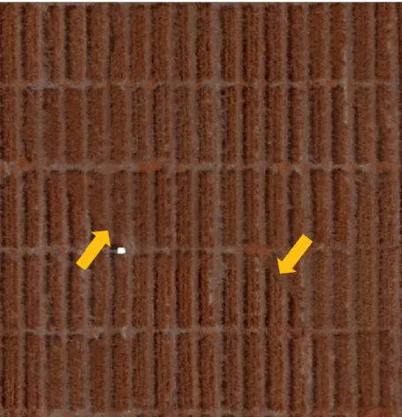
calibration panel and their corresponding mean reflectance values at the spectral region of Canon S100 wavebands (B: 400-495, G: 490-550, NIR: 680-760). ... 49 Figure 4 An example of artifact in the orthomosaic generated by Mosaic blending method from

IRIS+ aerial imagery. The yellow arrows point to two locations in the orthomosaic where artifacts from merging different original images are evident. ... 50 Figure 5 Results of different plot extraction method overlay on a subset of plots from IRIS+

calibrated orthomosaic. a) simple-grid plots, b) field-map based method, c) image

classification approach and an example of misclassification; this example confirms the need of post processing for image classification method. ... 51 Figure 6 Linear relation between GNDVI from Canon S100 and BER GNDVI from

spectroradiometer. Sample plot GNDVI values were extracted from calibrated orthomosaic of Canon S100 imagery, IRIS+ and band equivalent GNDVI for Canon S100 camera

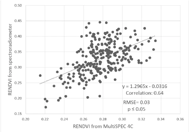
calculated from ASD spectroradiometer readings for 280 sample plots. ... 52 Figure 7 Scatterplot of the plot-level RENDVI from MultiSpec 4C imagery vs

spectroradiometer. Plot-level RENDVI were extracted from orthomosaic generated from MultiSPEC 4C camera imagery using field-map based plot extraction method, and Band equivalent RENDVI for Spec 4C calculated from spectroradiometer reading for 280 sample plots. ... 53 Figure 8 (A) Mapping yield values in drought environment shows the spatial variation across the

(13)

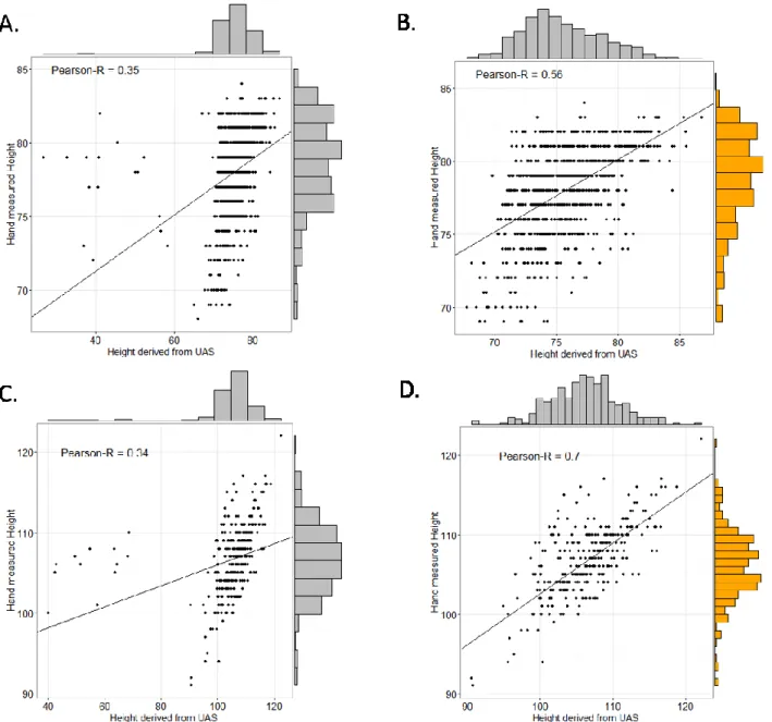
in irrigated environment shows patches of spatial variation across the field, although less variation compares to the yield in drought. (D) map of GNDVI values for irrigated in March 10, 2016. ... 88 Figure 9 (A) Correlation between 900 manual height data collected from the drought

environment, and the 900 height extracted from UAS (r= 0.35). (B) The correlation improves after removing the data points with high standard variations from heights

extracted from UAS imagery (r= 0.56). (C) Pairwise correlation between 300 manual height data from the first rep of each trial in irrigated environment, and corresponding height extracted from UAS (r= 0.34). (D) The correlation improves after removing the data points with high standard variations (r= 0.7). ... 89 Figure 10 Prediction accuracy between predicted grain yield and observed grain yield for

drought and irrigated environment using principal component regression and geographically weighted regression. GWR resulted in higher prediction accuracies compared to principal component regression (r=0.74 for drought environment using GWR versus r=0.48 suing PCR, and for irrigated environment, r=0.46 using GWR approach versus r=0.32 using PCR analysis) ... 90 Figure 11 Modified moving window search for A) Drought and B) Irrigated environment. The

plots are arranged based on their location on the ground using their Latitude-Longitude coordinates. The search window is a circular window with a defined radius based on the distance of the neighboring plots from each other. C) the search window of moving grid package before adjustment, number of neighboring plots can be defined on each row and column. The circles in the field represent the true centroid of each wheat plots extracted from aerial imagery. The distance between center of wheat plots in irrigated trials is approximately 1.6 m horizontally, and 3.5 m vertically. This distance for drought environment is 1.3 m and 4.6 m. These distances vary throughout the field due to the

presence of possible mistakes in planting. ... 118 Figure 12 Z scores are standard deviations. For example, a Z score of +2.5, means that the result

is 2.5 standard deviations. Both Z scores and p-values are associated with the standard normal distribution. ... 119 Figure 13 Z score map of A) Drought environment, B) Irrigated Environment. Z score values

(14)

environments, with inverse distance conceptualization of spatial relationships and

accounting for 8 neighbors for each plot. The circles in the field represent the true centroid of each wheat plots extracted from aerial imagery. ... 120 Figure 14 Temporal and spatial pattern analysis of high-throughput phenotyping data extracted

from UAS imagery captured at various time points after heading. A) Contour map of GNDVI values obtained on March 10, 2016 from irrigated trials. Spatial variation is observable as high values are clustered in patches on the right side of the field. B) GNDVI map, March 15, 2016, irrigated field. The trend of variation has changed from the last time point, but still high across the field. C) GNDVI map from April 8, 2016, the trend of GNDVI values has changed in this data set, patches of high values are scattered across the field. D) Contour map of GNDVI values extracted from UAS imagery from March 2nd, 2016, in drought trials. Spatial variation is observable in patches across the field. E) GNDVI values from March 10, 2016, the trend has changed, fewer clusters of high values of

GNDVI can be observed on the left side of the field, although the pattern on the right side has slight change. F) GNDVI values extracted from March 14 imagery; the spatial variation is very strong in the field, patches of high values on the left side. Slight change of low value clusters on the right side of the field is observable compare to March 10 data set... 121 Figure 15 Plot residuals along the field for drought trials. The color scale shows the value of

residual effects as indicated: A) Distribution of residual values of yield in drought environment from moving grid adjustment B) Residuals from modified moving grid approach for Yield values, drought environment, C) Plot residuals along the field for GNDVI values, in drought environment from moving grid approach, GNDVI values were extracted from UAS imagery captured on March 10, 2016 D) Residuals for GNDVI values from March 10, 2016, drought from modified moving grid approach. ... 122 Figure 16 Plot residuals along the field for irrigated trials. The color scale shows the value of

residual effects as indicated: A) Distribution of residuals for yield values in irrigated environment using moving grid adjustment B) Residuals from modified moving grid approach for Yield values, drought environment, C) Distribution of residuals for GNDVI values, in drought environment using moving grid adjustment, GNDVI values were

(15)

Figure 17 Broad sense heritability within environment and trial. The broad sense heritability was calculated for GNDVI values for each date and yield values in irrigated environment, the average H2 has increased after spatial adjustment for all the GNDVI values, and for yield. The error bars show the standard deviations across all the trials. ... 124 Figure 18 The broad sense heritability was calculated for GNDVI values for each date and yield

values in drought environment. H2 has increased after spatial adjustment for all the GNDVI values, and yield. The error bars show the standard deviations across all the trials. ... 125 Figure 19 A foldable gray scale reference panel, used in the field for radiometric calibration as

well as white balance correction ... 128 Figure 20 Surveying ground control points (GCPs) in the field using RTK GPS. Before the start

of HTP 10-13 GCPs were uniformly distributed in the field. ... 129 Figure 21 IRIS+ (3D Robotics, Inc, Berkeley, CA 94710, USA) a low cost UAV, carrying

modified NIR Canon S100 ... 130 Figure 22 Location of the study area with drought wheat trials in 2016 on the Norman E Borlaug

Experiment Station at Ciudad Obregon, Sonora. ... 130 Figure 23 Location of the study area with irrigated wheat trials in 2016 on the Norman E Borlaug Experiment Station at Ciudad Obregon, Sonora. ... 131 Figure 24 Orthomosaic of UAS imagery captured on March 10, 2016 from drought trials,

Norman E Borlaug Experiment Station at Ciudad Obregon, Sonora. 13 GCPs were

uniformly distributed across the field before data collection. ... 132 Figure 25 GNDVI map of drought trials, calculated from UAS imagery captured on March 2nd,

2016, which reveal the relative greenness of wheat plots. ... 133 Figure 26 GNDVI map of drought trials, calculated from UAS imagery captured on March 10th,

2016. Low GNDVI values (Less green and more red) indicate a low fraction or absence of green plants on the surface. ... 134 Figure 27 GNDVI map of drought trials, calculated from UAS imagery captured on March 14th,

(16)

List of Tables

Table 1 Sensor specification. ... 44 Table 2 Flight information using IRIS+ (multirotor) and eBee Ag (fixed wing) UASs, on May 6,

2015, at CIMMYT, Cd Obregon, Mexico. * RAW images of Canon S100 were converted to 16 bits TIFF imagery after pre-processing in Canon Digital Photo Professional software (DPP). ... 45 Table 3 Correlation analysis between mean GNDVI values extracted from raw Canon S100

digital number values, Calibrated Canon S100 digital number values and corresponding band equivalent reflectance (BER) GNDVI values from the spectroradiometer using

different plot boundary extraction method... 45 Table 4 Calculated vegetation indices for each camera, based on their spectral bands and

correlation between vegetation index values extracted from UAS imagery and band

equivalent reflectance values from Spectroradiometer. The values from Canon S100 values are before applying modified empirical line correction method. ... 46 Table 5 Correlation between repeated measurements from Handheld ASD for two different

vegetation indices. Four measurements were taken on each of 280 plots. To determine repeatability, the first two measurements were averaged and correlated to the average of the second two measurements on a per plot basis across all plots. The VIs presented are band equivalent indices for the Canon S100 (Green Normalized Difference Vegetation Index; GNDVI) and MultiSpec 4C (Red-edge Normalized Difference Vegetation Index: RENDVI) used in this study. ... 46 Table 6 Broad-sense heritability in 11 trials for vegetation indices and grain yield. The VIs

derived from the Canon S100 had a higher heritability than the MultiSpec 4C for nine out of eleven trials (shown in bold font). ... 47 Table 7 Sensor specifications for each instrument used for spectral data collection. ... 84 Table 8 Flight information using unmanned aerial system high-throughput phenenotyping

platform (IRIS+ and modified Canon S100), at CIMMYT, Ciudad Obregon, Mexico, 2016. ... 84

(17)

Table 9 Vegetation indices calculated for each day of data measurements using a modified Canon S100. ... 85 Table 10 Broad-sense heritability in 10 trials for vegetation indices and grain yield. The VIs

extracted from Canon S100 at three time points during the growing season for Drought and irrigated environment. In irrigated all the VIs derived from the Canon S100 had higher heritability than the final grain yield. ... 86 Table 11 Flight information using unmanned aerial vehicle high-throughput phenotyping

platform (IRIS+ and modified Canon S100), at CIMMYT, Ciudad Obregon, Mexico, 2016. ... 117

(18)

Acknowledgements

To my family. Obviously.

To Dr. Poland who gave me a unique opportunity. To my advisers.

To Poland lab, technicians, scientists, and support staff who made these research opportunities accessible to me.

(19)

Chapter 1 - Introduction

A plant phenotype is a set of structural, morphological, physiological, and performance-related traits of a given genotype in a defined environment (Granier & Vile 2014). The phenotype results from the interactions between a plant's genes and environmental factors. Plant phenotyping involves a broad range of plant measurements such as growth development, canopy architecture, physiology, disease and pest response and yield. Traditional phenotyping methods often rely on simple tools like rulers and other measuring devices, along with significant amounts of manual work, to extract the desired trait data. Compared to advanced genotyping methods such as the latest sequencing technologies, traditional phenotyping methods are time-consuming, labor-intensive, and cost-inefficient. This limits our ability to quantitatively understand how genetic traits are related to plant growth, environmental adaptation, and yield.

Great interest in plant high-throughput phenotyping (HTP) techniques has arisen, in the past several years. HTP is an assessment of plant phenotypes on a scale and scope not achievable with traditional methods such as visual scoring and manual measurements (Dhondt et al. 2013). HTP techniques use sensor systems and automated computer algorithms to extract phenotypic traits for large genetic mapping populations using non-destructive and non-invasive sampling methods. To be useful to breeding programs, HTP methods must be amenable to plot sizes, experimental designs and field conditions in these programs. This requires evaluating a large number of lines within a short time span, methods that are lower cost and less labor intensive than current techniques, and accurately assessing and making selections in large populations consisting of thousands to tens-of-thousands of plots (Sanchez, A et al. 2014; Haghighattalab et al. 2016). Use of information technologies such as remote sensing and computational tools are necessary to

(20)

rapidly identify the growth responses of genetically distinct plants in the field and link these responses to individual genes.

The extraction of data via HTP platforms requires a series of discrete steps that must be reliably executed in sequence. Such a set of steps is referred to as a "pipeline".

In recent years, most focused has been done on automation of data acquisition using a robotic vehicle with imaging systems and sensors. Less well-developed are data pipelines that automate data storage, processing, and analysis of the data extracted from these phenotyping platforms (White et al. 2012). Therefore, a slow manual collection of small amounts of data will get replaced by a slow manual management of large amounts of automatically-collected data unless we develop an automatic data analysis pipeline.

To address this challenge, we describe here and the chapters that follow a semi-automated HTP analysis pipeline using an unmanned aerial vehicle (UAV) platform, which will improve the capability of breeders to assess great numbers of lines in field trials. Then we will use remote sensing and geographic information (GIS) techniques to predict grain yield using the information extracted from UAS imagery, and finally, we will adjust the data, using the geostatistical approaches, for the spatial variation in the field.

This dissertation focuses on the areas in which plant phenotyping can be improved and how remote sensing and GIS can be incorporated into breeding programs. Some of the problems and panaceas investigated are: 1.) Development of a semi-automated HTP analysis pipeline using a low cost

(21)

unmanned aerial system (UAS) platform, and 2.) within-season grain yield prediction using spatio-temporal unmanned aerial systems imagery 3.) spatial adjustment of HTP data extracted from UAS imagery of field trial in wheat breeding nurseries.

Pipeline Development

Multispectral remote sensing plays a key role in precision agriculture due to its ability to represent crop growth condition on a spatial and temporal scale as well as its cost effectiveness.

In recent years, there has been increased interest in ground-based and aerial HTP platforms, particularly for applications in breeding and germplasm evaluation activities (Deery et al. 2014; Fiorani & Schurr 2013; Walter et al. 2015). Ground-based phenotyping platforms include modified vehicles using proximal sensing sensors (Busemeyer et al. 2013; Sanchez, A et al. 2014; Crain et al. 2015).

One of the emerging technologies in aerial based systems is UAV, which has undergone a remarkable development in recent years and is now a robust sensor-bearing platform for various agricultural and environmental applications (Dunford et al. 2009; Chapman et al. 2014). UAVs can cover an entire research site in a very short time, giving a rapid evaluation of the whole field and individual plots while minimizing the environment effects such as wind, cloud cover, and solar radiation. UAVs with sensors enable measuring with high spatial and temporal resolution, and capable of generating useful information for plant breeding programs.

(22)

With the introduction of HTP through UAV equipped with sensors, breeding programs can rapidly and reliably collect phenotypic data with minimal labor costs. This lowering of labor cost constraints allows for breeders to increase the number of lines assessed, thereby increasing the chance of achieving greater numbers of superior lines.

Recent advances in platform design, as well as the ability to the production of thousands of imagery and geo-referencing, and mosaicking the images, and extracting useful information from the imagery requires a workflow to execute HTP with UAS as a conventional tool in plant breeding. Additionally, developing efficient and easy-to-use pipelines to process HTP data and disseminate associated algorithms are necessary when dealing with big data. The primary objective of chapter 2 was to develop and validate a pipeline for processing data obtained by consumer grade digital cameras using a low-cost UAS to evaluate small plot field-based research typical of plant breeding programs.

Grain Yield Prediction

The primary objective of chapter 3 was to determine whether an accurate remote sensing based method could be developed to monitor plant growth and estimate grain yield using aerial spatio-temporal imagery in small plot wheat nurseries.

Multispectral sensors significantly help in exploring the relationships between crop biophysical data with crop production and yield. Many empirical relationships have been established in the past between spectral vegetation indices and crop growth rates through ground sampling or by using crop growth yield models. These relationships are then used by the crop growers, and

(23)

breeders to estimate the expected yield of crops within season, to make crop management and production related decisions for maximizing field productivity and market gains.

To examine the value of UAS in plant breeding and the data derived from the imagery, chapter 3 looks at how HTP measurements can be collected throughout the growing season, how geostatistical methods can be used to add value to data taken at multiple times throughout the growing season and predict grain yield. The purpose of this research is to evaluate the performance of geographically weighted models in predicting grain yields at plot level in breeding nurseries.

Spatial Adjustment

The introduction of geographic information system (GIS), global positioning systems (GPS) and remote sensing in agriculture, has resulted in more accurate and efficient mapping of field variability.

The phenotypes are determined by the genetics of each entry in the nursery but also influenced by the spatial variation across the field along with the variation of genotypic values. To improve the accuracy of selections, breeder needs to account for non-heritable environmental variation in the form of spatial field effects. To improve the accuracy of selections, breeder needs to account for environmental variation in the form of spatial field effects. These variations are caused by multiple environmental factors that can vary across a field such as soil fertility, soil type, moisture holding capacity, and also many human-made variations such as irrigation system, the direction of cultivation/harvesting, and previous crop cycles (Funda et al. 2007; Bos 2008; Sarker & Singh 2015).

(24)

The goal of chapter 4 is to evaluate the use of moving grid, integrate with spatial information extracted from UAS images to adjust for environmental variation in high throughput phenotypic data and yield of a large wheat breeding nursery.

The eye in the sky

Aerial and NIR imagery have been used for more than 50 years to monitor crop growth. In recent years, the application of unmanned aerial systems for crop studies and precision agriculture has been gaining importance due to the improvements in the spatial and spectral resolution of the sensors, and also the smaller size of the cameras to be mounted on these platforms.

Recent studies have shown the potential of UAS in monitoring of plant growth for different crops such as wheat, corn, cotton, sorghum, rice, and so on (Swain et al. 2010; Haghighattalab et al. 2016; Neely et al. 2016; Hunt et al. 2008; Lelong et al. 2008).

The pipeline developed in this study is applicable to any crop types. GW regression as described in chapter 3 can also be used to predict grain yield for any other crops, and also can be used to predict grain yield from multiyear data set as long as data is provided from the same exact location. The spatial adjustment technique developed and explained in chapter 4, can be applied to any breeding field with spatial variation.

(25)

REFERENCE

Haghighattalab, A. et al., 2016. Application of unmanned aerial systems for high throughput phenotyping of large wheat breeding nurseries Application of unmanned aerial systems for high throughput phenotyping of large wheat breeding nurseries. Plant Methods, (August). Available at: "http://dx.doi.org/10.1186/s13007-016-0134-6.

Hunt, E.R. et al., 2008. Remote Sensing of Crop Leaf Area Index Using Unmanned Airborne Vehicles. October, 17, pp.18–20. Available at:

http://www.asprs.org/publications/proceedings/pecora17/0018.pdf.

Lelong, C.C.D. et al., 2008. Assessment of unmanned aerial vehicles imagery for quantitative monitoring of wheat crop in small plots. Sensors, 8(5), pp.3557–3585.

Neely, L. et al., 2016. Unmanned Aerial Vehicles for High- Throughput Phenotyping and Agronomic Research. PLoS ONE, 11(7), pp.1–26.

Swain, K.C., Thomson, S.J. & Jayasuriya, H.P.W., 2010. Adoption of an Unmanned Helicopter for Low-Altitude Remote Sensing to Estimate Yield and Total Biomass of a Rice Crop. , 53(1). Available at: http://elibrary.asabe.org/abstract.asp?aid=29493&t=3.

(26)

Chapter 2 - Application of Unmanned Aerial Systems for High

Throughput Phenotyping of Large Wheat Breeding Nurseries

This chapter has been published as following journal article:

Haghighattalab A, González Pérez L, Mondal S, Singh D, Schinstock D, Rutkoski J, Ortiz-Monasterio I, Singh RP, Goodin D, Poland J: Application of unmanned aerial systems for high throughput phenotyping of large wheat breeding nurseries. Plant Methods 2016, 12:1–15

Abbreviations

BER, Band Equivalent Reflectance; CIMMYT, International Maize and Wheat

Improvement Center; DEM, Digital Elevation Model; DN, Digital Number; DPP, Digital Photo Professional; ENDVI, Enhanced Normalized Difference Vegetation Index; FWHM, Full Width at Half Maximum; GCP, Ground Control Points; GIPVI, Infrared Percentage Vegetation Index; GNDVI, Green Normalized Difference Vegetation Index; GSD, Ground Sampling Distance; HTP, High-throughput Phenotyping; LAI, Leaf Area Index; NDVI, Normalized Difference Vegetation Index; NIR, Near Infrared; RENDVI, Red-edge Normalized Difference Vegetation Index; RMSE, Root Mean Square Error; SIFT, Scale-invariant Feature Transform; UAS, Unmanned Aerial System; UAV, Unmanned Aerial Vehicle; VI, Vegetation Index

(27)

ABSTRACT

Background: Low cost unmanned aerial systems (UAS) have great potential for rapid proximal measurements of plants in agriculture. In the context of plant breeding and genetics, current approaches for phenotyping a large number of breeding lines under field conditions require substantial investments in time, cost, and labor. For field-based high-throughput phenotyping (HTP), UAS platforms can provide high-resolution measurements for small plot research, while enabling the rapid assessment of tens-of-thousands of field plots. The objective of this study was to complete a baseline assessment of the utility of UAS in assessment field trials as commonly implemented in wheat breeding programs. We developed a semi-automated image-processing pipeline to extract plot level data from UAS imagery. The image dataset was processed using a photogrammetric pipeline based on image orientation and radiometric

calibration to produce orthomosaic images. We also examined the relationships between vegetation indices (VIs) extracted from high spatial resolution multispectral imagery collected with two different UAS systems (eBee Ag carrying MultiSpec 4C camera, and IRIS+ quadcopter carrying modified NIR Canon S100) and ground truth spectral data from hand-held

spectroradiometer.

Results: We found good correlation between the VIs obtained from UAS platforms and ground-truth measurements and observed high broad-sense heritability for VIs. We determined radiometric calibration methods developed for satellite imagery significantly improved the precision of VIs from the UAS. We observed VIs extracted from calibrated images of Canon S100 had a significantly higher correlation to the spectroradiometer (r = 0.76) than VIs from the

(28)

MultiSpec 4C camera (r = 0.64). Their correlation to spectroradiometer readings was as high as or higher than repeated measurements with the spectroradiometer per se.

Conclusion: The approaches described here for UAS imaging and extraction of proximal sensing data enable collection of HTP measurements on the scale and with the precision needed for powerful selection tools in plant breeding. Low-cost UAS platforms have great potential for use as a selection tool in plant breeding programs. In the scope of tools development, the pipeline developed in this study can be effectively employed for other UAS and also other crops planted in breeding nurseries.

KEY WORDS

unmanned aerial vehicles / systems (UAV / UAS) wheat high-throughput phenotyping remote sensing GNDVI Plot extraction

(29)

INTRODUCTION

In a world of finite resources, climate variability, and increasing populations, food security has become a critical challenge. The rates of genetic improvement are below what is needed to meet projected demand for staple crops such as wheat [1]. The grand challenge remains in connecting genetic variants to observed phenotypes followed by predicting phenotypes in new genetic combinations. Extraordinary advances over the last 5-10 years in sequencing and genotyping technology have driven down the cost and are providing an abundance of genomic data, but this only comprise half of the equation to understand the

function of plant genomes and predicting plant phenotypes [2, 3]. High throughput phenotyping (HTP) platforms could provide the keys to connecting the genotype to phenotype by both

increasing the capacity and precision and reducing the time to evaluate huge plant populations. To get to the point of predicting the real-world performance of plants, HTP platforms must innovate and advance to the level of quantitatively assessing millions of plant phenotypes. To contribute to this piece of the challenge, we describe here a semi-automated HTP analysis pipeline using a low cost unmanned aerial system (UAS) platform, which will increase the capacity of breeders to assess large numbers of lines in field trials.

A plant phenotype is a set of structural, morphological, physiological, and performance-related traits of a given genotype in a defined environment [4]. The phenotype results from the interactions between a plant’s genes and environmental (abiotic and biotic) factors. Plant phenotyping involves a wide range of plant measurements such as growth development, canopy architecture, physiology, disease and pest response and yield. In this context, HTP is an

(30)

with traditional methods [5], many of which include visual scoring and manual measurements. To be useful to breeding programs, HTP methods must be amenable to plot sizes, experimental designs and field conditions in these programs. This entails evaluating a large number of lines within a short time span, methods that are lower cost and less labor intensive than current techniques, and accurately assessing and making selections in large populations consisting of thousands to tens-of-thousands of plots. To rapidly characterize the growth responses of genetically different plants in the field and relate these responses to individual genes, use of information technologies such as proximal or remote sensing and efficient computational tools are necessary.

In recent years, there has been increased interest in ground-based and aerial HTP platforms, particularly for applications in breeding and germplasm evaluation activities [6–8]. Ground-based phenotyping platforms include modified vehicles deploying proximal sensing sensors [9–12]. Measurements made at a short distance with tractors and hand-held sensors that do not necessarily involve measurements of reflected radiation, are classified as proximal sensing. Proximal, or close-range sensing, is expected to provide higher resolution for phenotyping studies as well as allowing collection of data with multiple view-angles,

illumination control and known distance from the plants to the sensors [13]. However, these ground-based platforms do have limitations mainly on the scale at which they can be used, limitations on portability and time required to make the measurements in different field locations.

(31)

As a complement to ground-based platforms, aerial-based phenotyping platforms enable the rapid characterization of many plots, overcoming one of the limitations associated with ground-based phenotyping platforms. There is a growing body of literature showing how these approaches in remote and proximal sensing enhance the precision and accuracy of automated high-throughput field based phenotyping techniques [14–16]. One of the emerging technologies in aerial based platforms is UAS, which have undergone a remarkable development in recent years and are now powerful sensor-bearing platforms for various agricultural and environmental applications [17–21]. UAS can cover an entire experiment in a very short time, giving a rapid assessment of all of the plots while minimizing the effect of environmental conditions that change rapidly such as wind speed, cloud cover, and solar radiation. UAS enables measuring with high spatial and temporal resolution capable of generating useful information for plant breeding programs.

Different types of imaging systems for remote sensing of crops are being used on UAS platforms. Some of the cameras used are RGB, multispectral, hyperspectral, thermal cameras, and low cost consumer grade cameras modified to capture near infrared (NIR) [2, 9, 21–23]. Consumer grade digital cameras are widely used as the sensor of choice due to their low cost, small size and weight, low power requirements, and their potential to store thousands of images. However, consumer grade cameras often have the challenge of not being radiometrically

calibrated. In this study, we evaluated the possibility of using traditional radiometric calibration methods developed for satellite imagery to address this issue.

(32)

Radiometric calibration accounts for both variations from photos within an observation day along with changes between different dates of image. The result of radiometric calibration is a more generalized and, most importantly, repeatable, method for different image processing techniques (such as derivation of VIs, change detection, and crop growth mapping) applied to the orthomosaic image instead of each individual image in a dataset. There are well-established radiometric calibration approaches for satellite imagery. However, these approaches are not necessarily applicable in UAS workflows due to several factors such as conditions of data acquisition during the exact time of image capture using these platforms.

Empirical line method is a technique often applied to perform atmospheric correction to convert at-sensor radiance measurements to surface reflectance for satellite imagery, although this technique can be modified to apply radiometric calibration and convert digital numbers (DNs) to reflectance values [24]. The method is based on the relationship between DNs and surface reflectance values measured from calibration targets located within the image using a field spectroradiometer. The extracted DNs from the imagery are then compared with the field-measured reflectance values to calculate a prediction equation that can be used to convert DNs to reflectance values for each band [25].

Advances in platform design, production, standardization of image geo-referencing, mosaicking, and information extraction workflow are needed to implement HTP with UAS as a routine tool in plant breeding and genetics. Additionally, developing efficient and easy-to-use pipelines to process HTP data and disseminate associated algorithms are necessary when dealing with big data. The primary objective of this research was to develop and validate a pipeline for

(33)

processing data captured by consumer grade digital cameras using a low cost UAS to evaluate small plot field-based research typical of plant breeding programs.

MATERIALS and METHODS

Study Area

The study was conducted at Norman E Borlaug Experiment Station at Ciudad Obregon, Sonora, Mexico (Figure 1). The experiment consisted of 1092 advanced wheat lines distributed in 39 trials, each trial consisting of 30 entries. Each trial was arranged as an alpha lattice with three replications. The experimental units were 2.8m x 1.6m in size consisting of paired rows at 0.15m spacing, planted on two raised beds spaced 0.8m apart. The trials were planted later than optimal on February 24, 2015 to simulate heat stress with temperatures expected to be above optimum for the entire growing season (the local recommended planting date is November 15 to December 15). Irrigation and nutrient levels in the heat trials were maintained at optimal levels, as well as weed, insect and disease control. Grain yield was obtained by using a plot combine harvester.

Platforms and Cameras

We evaluated two unmanned aerial vehicles (UAV); the IRIS+ (3D Robotics, Inc, Berkeley, CA 94710, USA) and eBee Ag (senseFly Ltd., 1033 Cheseaux-Lausanne, Switzerland).

The IRIS+ is a low cost quadcopter UAV with a maximum payload of 400 g. The open-source Pixhawk autopilot system was programmed for autonomous navigation for the IRIS+

(34)

based on ground coordinates and the ‘survey’ option of Mission Planner (Pixhawk sponsored by 3D Robotics, www.planner.ardupilot.com). The IRIS+ is equipped with an uBlox GPS with integrated magnetometer. A Canon S100 modified by MaxMax (LDP LLC, Carlstadt, NJ 07072, USA, www.maxmax.com) to Blue-Green-NIR (400-760nm) was mounted to the UAV with a gimbal designed by Kansas State University. The gimbal compensates for the UAV movement (pitch and roll) during the flight to allow for nadir image collection.

The eBee Ag, designed as a fixed wing UAV for application in precision agriculture has a payload of 150 g. This UAV was equipped with MultiSpec 4C camera developed by Airinov (Airinov, 75018 Paris, France, www.airinov.fr/en/uav-sensor/agrosensor/) and customized for the eBee Ag. It contains four distinct bands with no spectral overlap (530-810nm): green, red, red-edge, and near infrared bands, and is controlled by the eBee Ag autopilot during the flight.

For ‘ground-truth’ validation, spectral measurements were taken using ASD VNIR handheld point-based spectroradiometer (ASD Inc., Boulder, CO, http://www.asdi.com/) with a wavelength range of 325 nm – 1075 nm, a wavelength accuracy of ±1 nm and a spectral

resolution of <3 nm at 700 nm with a fiber optics of 25° (aperture) full conical angle. The instrument digitizes spectral values to 16 bits. Table 1 summarizes the specification for the cameras and sensor used in this study.

Ground Control Points

In order to geo-reference the aerial images, at the beginning of the season ten ground control points (GCPs) were distributed across the field. The GCPs were 25 cm x 25 cm square

(35)

white metal sheets mounted on a 50 cm post. The GCPs were white to provide easy

identification for the image processing software. The GCP coordinates were measured with a Trimble R4 RTK GPS, with a horizontal accuracy of 0.025 m and a vertical accuracy of 0.035 m. These targets were maintained throughout the crop season to enable more accurate

geo-referencing of UAS aerial imagery and overlay of measurements from multiple dates.

Reflectance Calibration Panel

For radiometric calibration, spectra of easily recognizable objects (e.g. gray scale calibration board) are needed. A black-gray-white grayscale board with known reflectance values was built and placed in the field during flights for further image calibration. This

grayscale calibration panel met the requirements for further radiometric calibration including 1) the panel was spectrally homogenous, 2) it was near Lambertian and horizontal, 3) it covered an area many times larger than the pixel size of the Canon S100, and 4) covered a range of

reflectance values [25].

The calibration panel used in this study had 6 levels of gray from 0% being white and 100% being black, printed on matte vinyl. This made it possible to choose several dark and bright regions in the images to provide a more accurate regression for further radiometric calibration analysis. Photos of the calibration panel were taken in the field before a UAS flight using the same Canon S100 NIR camera mounted on the IRIS+. Using an ASD

spectroradiometer on a sunny day, the spectral reflectance was measured of the panel at a ﬁxed altitude of 0.50 m from different angles.

(36)

Field Data Collection

At the study site, image time series were acquired using IRIS+ and Canon S100 camera during the growing season as evenly spaced as possible, depending on the weather condition; April 10, April 22, April 28, May 6, and May 18, 2015.

Field data measurements for the experiment in this study included 1) IRIS+ carrying modified NIR Canon S100, and 2) eBee Ag carrying MultiSpec 4C camera, and 3) spectral reflectance measurements using handheld ASD spectroradiometer collected on May 6, 2015 when the trials were at mid grain filling. We took all field measurements within one hour around solar noon to minimize variation in illumination and solar zenith angle [26]. This limited the number of plots we could measure using handheld spectroradiometer to 280 plots. Four spectra per plot were taken with the beam of the fiber optics placed at 0.50 m over the top of the canopy with a sample area of 0.04 m2. Due to this very small sampling area, great care was taken in data collection to make sure the measured spectral responses were only from the crops.

Both the eBee and IRIS+ were able to image a much larger area in the same time frame. Each system was flown using a generated autopilot path that covered the 2 ha experiment area with an average of 75% overlap between images (Table 2).

For the IRIS+ with Canon S100, all images were taken in RAW format (.CR2) to avoid loss of image information. The Canon S100 settings were TV mode, which allowed setting of a constant shutter speed. The aperture was set to be auto-controlled by the camera to maintain a good exposure level, and ISO speed was set to Auto with a maximum value of 400 to minimize noise in the images. Focus range was manually set to infinity. We used CHDK

(37)

(www.chdk.wkia.com) to automate Canon S100’s functionality by running intervalometer scripts off an SD card in order to take pictures automatically at intervals during flight. The CHDK script allowed the UAS autopilot system to send electronic pulses to trigger the camera shutter. The camera trigger was set at the corresponding distance interval during the mission planning for the desired image overlap.

The eBee MultiSpec 4C camera had a predefined setting by Sensefly; ISO and shutter speed was set to automatic, maximum aperture was set to f/1.8 and focal distance was fixed at 4 mm.

Developing an image processing pipeline for HTP

In this research, a UAS-based semi-automated data analyses pipeline was developed to enable HTP analysis of large breeding nurseries. Data analysis was primarily conducted using Python scripts [27, 28]. The dataset used to develop the image processing pipeline was

collected on May 6, 2015 with the IRIS+ flights carrying the modified NIR Canon S100 camera. In order to analyze hundreds of images taken by a UAS that represent the entire experiment area, we developed a semi-automated data analysis pipeline. The developed pipeline completed the following steps: 1) Image pre-processing, 2) Georeferencing and orthomosaic generation, 3) Image radiometric calibration, 4) Calculation of different VIs and 5) plot-level data extraction from the VI maps. The overall workflow of the developed pipeline is presented in Figure 2, and a detailed description of each segment is provided.

(38)

The RAW images of Canon S100 (.CR2 format) were pre-processed using Digital Photo Professional (DPP) software developed by Canon

(http://www.canon.co.uk/support/camera_software/). This software to convert RAW to Tiff also included lens distortion correction, chromatic aberration, and gamma correction. For white balance adjustment, we used the pictures of grayscale calibration panel taken during the flights. After pre-processing the images were exported as a tri-band 16-bit linear TIFF image.

Image Stitching and Orthomosaic Generation

We then generated a geo-referenced orthomosaic image using the TIFF images. There are several software packages for mosaicking UAS aerial imagery, all based around the scale-invariant feature transform algorithm (SIFT) algorithm for feature matching between images [29]. While there are slight differences between packages each performs the same operation namely loading photos; aligning photos; importing GCP positions; building dense point cloud; building digital elevation model (DEM); and finally generating the orthomosaic image. We used the commercial Agisoft PhotoScan package (Agisoft LLC, St. Petersburg, Russia, 191144) to automate the orthomosaic generation within a custom Python script. The procedure of

generating the orthomosaic using PhotoScan comprises five main stages 1) camera alignment, 2) importing GCPs and geo-referencing, 3) building dense point cloud, 4) building DEM and 5) generating orthomosaic [30].

For alignment, PhotoScan finds the camera position and orientation for each photo and builds a sparse point cloud model; the software uses the SIFT algorithm to find matching points of detected features across the photos. PhotoScan offers two options for pair selection: generic

(39)

and reference. In generic pre-selection mode, the overlapping pairs of photos are selected by matching photos using the lower accuracy setting. On the other hand, in reference mode the overlapping pairs of photos are selected based on the measured camera locations. We examined both methods to generate the orthomosaic and compared the results.

With aerial photogrammetry the location information delivered with cameras is

inadequate and the data does not align properly with other geo-referenced data. In order to do further spatial and temporal analysis with aerial imagery, we performed geo-referencing using GCPs. We used 10 GCPs evenly distributed around the orthomosaic image. Geo-referencing with GCPs is the step that still requires manual input.

The main source of error in georeferencing is performing the linear transformation matrix on the model. In order to remove the possible non-linear deformation components of the model, and minimizing the sum of re-projection error and reference coordinate misalignment, PhotoScan offers an optimization of the estimated point cloud and camera parameters based on the known reference coordinates [30].

After alignment optimization, the next step is generating dense point clouds. Based on the estimated camera positions PhotoScan calculates depth information for each camera to be

combined into a single dense point cloud [30]. PhotoScan allows creating a raster DEM file from a dense point cloud, a sparse point cloud or a mesh to represent the model surface as a regular grid of height values. Although most accurate results are calculated based on dense point cloud data.

(40)

The final step is orthomosaic generation. An orthomosaic can be created based on either mesh or DEM data. Mesh surface type can be chosen for models that are not referenced. The blending mode has two options (mosaic and average) to select how pixel values from different photos will be combined in the final texture layer. Average blending computes the average brightness values from all overlapping images to help reduce the effect of the bidirectional reflectance distribution function that is strong within low altitude wide-angle photography [31]. Blending pixel values using mosaic mode does not mix image details of overlapping photos, but uses only images where the pixel in question is located within the shortest distance from the image center. We compared these two methods by creating orthomosaic images using both mosaic and average mode.

Radiometric Calibration

After the orthomosaic was completed, we then performed radiometric calibration to improve the accuracy of surface spectral reflectance obtained using digital cameras. We applied empirical line correction to each orthomosaic within the data set using field measurements taken with the ASD. The relationship between image raw DNs and their corresponding reflectance values is not completely linear for all the bands for Canon S100 camera and most digital cameras (Figure 3). To relate remote sensing data to field-based measurements we used a modified empirical line method [32]. We used the grayscale calibration board combined with reflectance measurements from the ASD spectroradiometer to find the relationship between DNs extracted form Canon S100 and surface reflectance values measured from grayscale calibration board

(41)

using a field spectroradiometer. We then calculated the prediction equations for each band separately to convert DNs to reflectance values.

We calculated the mean pixel value of the calibration panel extracted from images for each band separately, and plotted against the mean band equivalent reflectance (BER) of field spectra [33, 34]. We found a linear relation between the natural logarithm of image raw DN values and their corresponding BER, although the relation between image raw DNs and their corresponding BER was not completely linear for all bands of Canon S100 (Figure 3). We derived the correction coefficient needed to fit uncalibrated UAS multispectral imagery to field-measured reflectance spectra. Using the correction coefficient for each band, we then performed this correction on the entire image.

With the corrected orthomosaic, a map showing the vegetation indices can be generated. The most used VIs derivable from a three-band multispectral sensor are: normalized difference vegetation index (NDVI), and green normalized difference vegetation index (GNDVI) (Table 4). NDVI is calculated from reflectance measurements in the red and NIR portion of the spectrum and its values range from −1.0 to 1.0. GNDVI is computed similarly to the NDVI, where the green band is used instead of the red band and its value ranges from 0 to 1.0. Like NDVI, this index is also related to the proportion of photosynthetically absorbed radiation and is linearly correlated with Leaf Area Index (LAI) and biomass [22, 35, 36].

(42)

Field Plot Extraction

In order to get useful information about each wheat plot in the field, we need to extract plot level data from the orthomosaic VI image. Individual wheat plot boundaries need to be extracted and defined separately from images with an assigned plot ID that defines their genomic type. We examined three approaches for extracting plot boundaries from the orthomosaic image: a simple grid based plot extraction, field-map based plot extraction, and image

classification/segmentation.

To apply a simple grid superimposed on top of the orthomosaic image we used the Fishnet function using Arcpy scripting in ArcGIS. This function creates a net of adjacent rectangular cells. The output is polygon features defining plot boundaries. Creating a fishnet requires two basic pieces of information: the spatial extent of the desired net, and the number of rows and columns. The number of rows and ranges (columns) and height and width of each cell in the fishnet can be defined by the user. The user can also define the extent of the grid by supplying both the minimum and maximum x- and y-coordinates.

The next method we evaluated in this study is a field-map based method. Experimental or field data are usually stored in a spreadsheet. To accomplish this, we reformatted the field map in order to represent the plots in the field; the first row of the excel sheet is the length (or width, depending on how plots are located in the field) of the plots, and the first column is the width (or length). Each cell in the excel sheet is the plot ID and other information regarding that particular plot available in the field map.

(43)

In this approach, first we created a KML file from the field map (.CSV) using Python [27], we generated polygon shapefiles with known size for each plot from KML file, and assigned plot ID to each plot using the field map. To define the geographic extent of the field, the python script has inputs for the coordinate of two points in the field: the start point of the first plot on the top right and the end point of the last plot on the bottom left. The script starts from the top right and builds the first polygon using the defined plot size, and skips the gap between plots and generates the next one until it gets to the last plot on the bottom left. In this approach the plot IDs are assigned automatically and simultaneously from the field map excel sheet. The most important advantage of this approach is that it can be generalized to other crop types as long as the field map is provided and the plots are planted in regular distance and have a consistent size within a trial.

The third method is to extract wheat plot boundaries from the orthomosaic image directly. To examine this method, we used the April 10 data set instead of May 6. The reason for choosing this set of data was that in this dataset we had the most distinguished features (e.g. vegetation vs. bare soil) in the image compared to the image data taken on May 6. We classified the GNDVI image created from the orthomosaic image into four classes: “Wheat”, “Shadow”, “Soil”, and a class named “Others” for all the GCP targets in the field. The class “shadow” stands for the shadow projected on the soil surface. In this supervised classification, we defined training samples and signature files for each defined class. After classifying the image, we merged the “Shadow”,” Soil” and “Others” classes together and ended up with two classes: “Wheat”, and “Non-wheat”. The classified image often needs further processing to clean up the

(44)

random noise and small isolated regions to improve the quality of the output. With a simple segmentation, we extracted wheat plot polygons from the image.

This method works best with high-resolution imagery taken at the beginning of the growing season when all the classes are clearly distinguishable from each other on the image. Otherwise time consuming post-processing is needed in order to separate the mixed classes.

To analyze the result of VI extraction from the orthomosaic, we used the zonal statistics plugin in the open source software QGIS. We calculated several values of the pixels of

orthomosaic (such as the average VI values, Min, Max, standard deviation, majority, minority and also the median of VI values for each plot and the total count of the pixels that are within a plot boundary), using the polygonal vector layer of plot boundaries generated by one of the methods above. We then merged the data from the field map spreadsheet (plot ID, entry

numbers, trial name, number of rep, number of block, row and column, and other information on planting) with the generated plots statistics.

Accuracy evaluation of different types of aerial imagery sensors and platforms To evaluate the accuracy and reliability of our low cost UAS and consumer grade camera, we calculated correlations between calibrated DN values from the orthomosaic images of Canon S100 and MultiSpec 4C camera and band equivalent reflectance (BER) of field spectra. For ground-truth evaluation we used the ASD Fieldspectro 2 spectroradiometer to measure

spectral reference of 280 sample plots after running the UAS within the time window of 1 hour around noon. The ASD spectroradiometer measures a wavelength range of 325 nm – 1075 nm, a

(45)

wavelength accuracy of ±1 nm and a spectral resolution of <3 nm at 700 nm (Table 1). Using the ASD, the top of canopy reflectance was measured approximately 0.5 m above the plants. To account for the very small field of view of this sensor, we constantly monitored the spectral response curves to avoid measuring mixed pixels in our samplings and we averaged four reflectance readings within each sample plots. Reflectance measurements were calibrated at every 15 plots using a white (99% reflectance) Spectralon calibration panel.

To evaluate the accuracy of each platform, we calculated the correlations between different VIs extracted from Canon S100 and VIs extracted from MultiSpec 4C compared to the BER of field spectra. We calculated BER for each camera separately by taking the average of all the spectroradiometer bands that are within the full width at half maximum (FWHM) of each instrument (Table 1). The Pearson correlation between the average VI values of the sample plots and field spectra for each platform was calculated. The resulting correlation coefficients were tested using a two-tail test of significance at the p ≤ 0.05 level. Accuracy assessment was based on computing the root mean square error (RMSE) for GNDVI image by comparing the pixel values of the reflectance image to the corresponding BER of field spectra at the sample sites not selected to generate the regression equations.

Broad-sense Heritability

Broad-sense heritability, commonly known as repeatability, is an index used by plant breeders and geneticists to measure precision of a trial [37–39]. The ratio of the genetic variance to the total phenotypic variance is broad-sense heritability (H2), which varies between 0 and 1. A heritability of 0 indicates there is no genetic variation contributing to phenotypic variation, and

(46)

H2 of 1 if the entire phenotypic variation is due to genetic variation and no environmental noise. For the purpose of comparing phenotyping tools and approaches, broad-sense heritability

calculated for measurements on a given set of plots under field conditions at the same point in time, is a direct assessment of measurement error as the genetics and environmental conditions are constant.

In order to assess the accuracy of the different HTP platforms, we calculated broad-sense heritability on an entry-mean basis for each individual trial and phenotypic sampling date on May 6, 2015. To calculate heritability, we performed a two steps process where we first

calculated the plot average and then fit a mixed model for replication, block and entry as random effects. Heritability was calculated from equation 1 [40].

𝐻2 ₌ 𝜎𝑔𝑒𝑛𝑜𝑡𝑦𝑝𝑖𝑐2

𝜎_{𝑝ℎ𝑒𝑛𝑜𝑡𝑦𝑝𝑖𝑐}2 =

𝜎_{𝑔𝑒𝑛𝑜𝑡𝑦𝑝𝑖𝑐}2

𝜎_{𝑔𝑒𝑛𝑜𝑡𝑦𝑝𝑖𝑐}2 +_{𝑟𝑒𝑝𝑙𝑖𝑐𝑎𝑡𝑖𝑜𝑛}𝜎𝑒𝑟𝑟𝑜𝑟2 (1)

Where𝜎_{𝑔𝑒𝑛𝑜𝑡𝑦𝑝𝑖𝑐}2 _{is genotypic variance and 𝜎}

𝑒𝑟𝑟𝑜𝑟2 is error variance.

RESULTS and DISCUSSION

Developing an image processing pipeline for HTP

To evaluate the potential of UAS for plant breeding programs, we deployed a low cost, consumer grade UAS and imaging system at multiple times throughout the growing season. Using the aerial imagery collected on May 6, we built a robust pipeline scripted in Python that facilitated image analysis and allowed a semi-automated image analysis algorithm to run with minimum user support. The only requirement for manual input in the processing pipeline is to

(47)

validate the GCP positions. This pipeline was tested on eight temporal datasets collected from IRIS+ flights over heat trials during the growing season.

The individual parameters selected during orthomosaic generation and plot extraction can have a large impact on the quality of the orthomosaic and subsequent data analysis. Because of the multiple parameter settings that users could choose, we investigated how changing various parameters would affect the data quality. To obtain more accurate camera position estimates, we selected higher accuracy at the alignment step. For pair selection mode, we chose reference since in this mode the overlapping pairs of photos are selected based on the estimated camera locations (i.e. from the GPS log of the control system). For the upper limit of feature points on every image to be taken into account during alignment stage, we accepted the default value of 40000. We imported positions for all of the ten GCPs available on the field to geo-reference the aerial images. The GCPs were also used in the self-calibrating bundle adjustment to ensure correct geo-location and to avoid any systematic error or block deformation. To improve georeferencing accuracy, we performed alignment optimization.

Finally, to generate orthomosaic, we tested the two methods of blending: mosaic and average. We found the orthomosaic generated by the mosaic method gives more quality for the orthomosaic and texture atlas than the average mode. On the other hand, mosaic blending mode generated artifacts in the image since it uses fewer images by selecting pixels with the shortest distance from the image center (Figure 4). We examined the correlation between orthomosaic generated from these two approaches and the ground truth data and found the averaging method has slightly higher correlation of 0.68 compared to mosaic method with the correlation of 0.65.

(48)

The 16 bit orthomosaic TIFF image was generated semi-automatically using python scripting in PhotoScan software with a resolution of 0.8 centimeters, matching the ground sampling distance (GSD) of the camera. Due to the short flight times (less than 20 minutes) and low flying altitude (30 meters above ground level), we assume there is no need for atmospheric corrections [28].

To convert DNs to reflectance values, a modified empirical approach was implemented using pixel values of IRIS+ aerial imagery and field-based reflectance measurements from handheld spectroradiometer. Calibration equations (2, 3, and 4) calculated from non-linear relationship between average field spectra and relative spectra response of each band separately were determined as:

𝑅𝑒𝑓𝑙𝑒𝑐𝑡𝑎𝑛𝑐𝑒_{𝐵𝑙𝑢𝑒} = − 𝑒𝑥𝑝 (−𝑙𝑜𝑔 (4.495970𝑒−01_{+ (3.191189𝑒}−05_{) ∗ 𝐷𝑁} 𝐵𝑙𝑢𝑒))) (2) (𝑟2 _{= 0.98 , P < 0.001)} 𝑅𝑒𝑓𝑙𝑒𝑐𝑡𝑎𝑛𝑐𝑒𝐺𝑟𝑒𝑒𝑛 = − 𝑒𝑥𝑝 (−𝑙𝑜𝑔 (4.705485𝑒−01+ (3.735676𝑒−05) ∗ 𝐷𝑁𝐺𝑟𝑒𝑒𝑛))) (3) (𝑟2 _{= 0.97, P < 0.001)} 𝑅𝑒𝑓𝑙𝑒𝑐𝑡𝑎𝑛𝑐𝑒_𝑁𝐼𝑅 = − 𝑒𝑥𝑝 (−𝑙𝑜𝑔 (1.197440𝑒+00_{+ (4.712299𝑒}−05_{) ∗ 𝐷𝑁} 𝑁𝐼𝑅))) (4) (𝑟2 _{= 0.94, P < 0.001)}

We applied each calibration equation to their corresponding band image and converted the image raw DNs into reflectance values.