To cite this version:
Lionel Fugon, J´
er´
emie Juban, Georges Kariniotakis. Data mining for wind power forecasting.
European Wind Energy Conference & Exhibition EWEC 2008, Mar 2008, Brussels, Belgium.
EWEC, 6 p., 2008.
<
hal-00506101
>
HAL Id: hal-00506101
https://hal-mines-paristech.archives-ouvertes.fr/hal-00506101
Submitted on 27 Jul 2010
HAL
is a multi-disciplinary open access
archive for the deposit and dissemination of
sci-entific research documents, whether they are
pub-lished or not.
The documents may come from
teaching and research institutions in France or
abroad, or from public or private research centers.
L’archive ouverte pluridisciplinaire
HAL, est
destin´
ee au d´
epˆ
ot et `
a la diffusion de documents
scientifiques de niveau recherche, publi´
es ou non,
´
emanant des ´
etablissements d’enseignement et de
recherche fran¸
cais ou ´
etrangers, des laboratoires
publics ou priv´
es.
Data mining for wind power forecasting
Lionel Fugon , J´
er´
emie Juban and George Kariniotakis
´
Ecole des Mines de Paris
B.P.207, F-06904 Sophia-Antipolis, France [email protected]; [email protected]
Abstract
Short-term forecasting of wind energy produc-tion up to 2-3 days ahead is recognized as a major contribution for reliable large-scale wind power integration. Increasing the value of wind generation through the improvement of predic-tion systems performance is recognised as one of the priorities in wind energy research needs for the coming years. This paper aims to evalu-ate Data Mining type of models for wind power forecasting. Models that are examined include neural networks, support vector machines, the recently proposed regression trees approach, and others. Evaluation results are presented for sev-eral real wind farms.
1
Introduction
Wind power has been undergoing a rapid devel-opment in recent years. Several countries have reached already a high level of installed wind power capacity, such as Germany, Spain and, Denmark, while others follow with fast rates of development. Such large-scale integration of wind power is challenging in terms of power sys-tem management. Indeed, wind is a variable re-source that is difficult to predict. As an example, traditionally, additional reserves are allocated to manage this uncertainty.
This increases the overall cost of the produced energy and limits the benefits of using such a renewable energy resource. A way of reducing the uncertainty associated to wind power pro-duction is to use forecasting tools. Development of such tools has been ongoing for more than 15 years [1]. These tools are multi-step ahead forecasting models that provide information for several horizons ahead. In the same way, the continuous improvement of computers and the constant increase in databases capacity permit-ted the development of a new scientific investi-gation field called Data Mining. Data Mining has been defined as ”the nontrivial extraction
of implicit, previously unknown, and potentially useful information from data (Fayyad, 1996)”. Several algorithmic techniques issued from Data Mining have already been adapted to the wind power forecasting [2] to provide a single expected value for each forecast horizon, called determin-istic, spot or point forecast.
The paper initially introduces the different al-gorithms used. Then the real-world data used to evaluate the models are presented. They are from French wind farms located in different ter-rain complexity and climatic conditions. Finally an evaluation and comparison of the models per-formance for each wind farm follows. The paper ends with some conclusions and remarks.
2
Data Mining Models Used
Data Mining encompasses different algorithms from many scientific fields (statistics, artifi-cial intelligence...) for building models (super-vised methods) : Y = φ(X) +ǫ where Y is the variable to predict or explain and X = (X1, X2, ..., Xn) represents the vector of the
n-explanatory variables.ǫis the error of the model. The aim is to approximate the function φ and minimize the error. For that purpose, we used both a linear and a non-linear approach.
2.1
Linear Models
Two versions of linear regression models have been considered: one base version, which is used as a simple reference model and a second one that includes interactions. Interactions basically consist in combining the input variables to cre-ate extra variables used in the same linear set-tings. This has the advantage of considering non-linearities while keeping a simple linear set-ting. However, this can enlarge considerably the dimension of the problem.
The linear model without interaction can be presented by the following formula:
where β = (β1, β2, ..., βn) represents the
vec-tor of linear regression coefficients to estimate. If we take account of different hypothesis onǫ
(such as i.i.d.), we approximate theβ-vector by least square minimization on the learning set:
n X i=1 yi−β0−β1xi 1 −β2xi 2 −...−βpxip =ky−Xβk2 (2) For the linear regression with interaction, cross products between variables are added to the input variables. Then, the same method is applied on this augmented input set.
2.2
Non-Linear Models
In this part, several non-linear models for wind power forecasting are considered. Such mod-els are better suited to account for the non-linearity of the wind to power conversion. First, neural networks are considered. Then, we con-sider models based on classification and regres-sion trees with a simple bagging verregres-sion and a more advanced version called random forest. Fi-nally, we present a last approach based on sup-port vector machines.
2.2.1 Neural Networks
A neural network is an ensemble of neurons (or nodes) connected along several levels called layer inspired by the structure of the human brain. It is generally composed of three layers of neurons, namely an input layer corresponding to explana-tory variables, an output layer that provides a response and one or several hidden layers. Neu-rons of a same layer are never connected between themselves.
Each neuron is affected a weight and passes signals based on a specific transfer function. The most used transfer function is the sigmoid, which receives as input a weighted linear combination of the output of the neurons of the previous layer:
s(θ) = 1
1 +exp(−θ) (3) withθ= ΣiβiXi.
The learning step of the neural network is based on a back-propagation algorithm. The principle is to adjust the different neuron weights progressively by back-propagating the error
pacity to model complex structures and account for non-linear relations between the explanatory variables and the output. Although, one of the main drawbacks, is that the final performance of a neural network is very sensitive to the design of the network. The choice of the number of hid-den layers and neurons contained in each layer is very important. For instance integrating a high number of neurons in the network permits to model more complex relations but can also lead to overfitting of the data and to poor out of sample performances. In this paper, in order to overcome this problem, a neural network ar-chitecture optimisation algorithm based on the parameter decay principle has been used (regu-larisation of the problem). A second drawback is that it is difficult to get insight on the learnt rela-tion simply by looking at the informarela-tion stored in the network. In this way, neural networks are generally considered as “black box” algorithms. 2.2.2 Random Forests
Bagging for Bootstrap Aggregating, is a method for generating an ensemble of models con-structed from samples bootstrap replicates [3]. These replicates are obtained by sampling uni-formly with replacement from the original sam-ples. The predictors are then combined by vot-ing for classification or averagvot-ing for regression [3]. The main advantage of averages of predic-tions from several models (like bootstrap sam-pling) is that it reduces the variance and predic-tion error.
The base method used in the models hereafter named “Bagging” and “Random Forest” is clas-sification and regression trees (CARTs) [4]. The goal of CARTs is to divide a sample of data using binary rules making the child nodes less hetero-geneous than the parent nodes. Once a tree is grown it is possible to extract information from the tree structure, which makes it also a tool for data analysis. The main advantages of CARTs is that it permits to perform a regression or a classification with high dimensional inputs and the major disadvantage of the later is that it is unstable i.e. a small change in the training sample can generate large changes in the learned predictor (classification or regression) [3]. The Bagging algorithm has been used in the specific case of binary tree and Random Forest is a ver-sion more sophisticated of Bagging because it adds a random input selection which consists in selecting at random, at each node, a small group
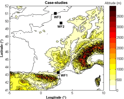
Figure 1: Map representing the location of the three considered wind farms WF1, WF2 and WF3. of input variables to split on. That way, the trees
built are more independent.
In the Random Forest approach, the condi-tional meanE[Y|X =x] is approximated by the averaged prediction ofK single trees, each con-structed with an i.i.d. vectorθk, k=1..K, which
represents the tree parameters defining how the tree is grown (e.g. split points).
The main drawbacks of these two algorithms are the important computing time of the learn-ing step and trees storage but the advantages are that an insensibility to overfitting thanks to out-of-bag error and few parameters to adjust. Moreover, Random Forest provides information about the frequency of variables appearance in trees, which can be used to determine the im-portance of each input variable.
2.2.3 Support Vector Machines (SVM) Support vector machines (SVM) are a recent supervised learning methods used, initially for classification, and generalized later for regres-sion. They are based on Vapnik’s research about learning theory. Support vector machines for classification are based on two ideas. First, a principle of maximum margin, which is the dis-tance maximizing the separation frontier and nearest elements called support vector. The learning step is the optimization of this frontier
and can be presented like a quadratic optimiza-tion problem. Secondly, the input dimension space is transformed into a higher dimensional space, thanks to a kernel function, where a max-imal separating hyperplane is constructed. The goal is to transform a complex (non-linear) low dimension problem into a simple (linear) high dimensional problem.
The SVM can be also used to predict a quan-titative variable: “the Support Vector method can also be applied to the case of regression, maintaining all the main features that charac-terise the maximal margin algorithm: a non-linear function is learned by a non-linear learning machine in a kernel-induced feature space while the capacity of the system is controlled by a pa-rameter that does not depend on the dimension-ality of the space” Cristianini and Shawe-Taylor (2000).
The main advantage of SVM is that the regu-larisation technique makes the model very resis-tant to overfitting. The main drawback of SVM is that the computing time required might be very high when compared to other non-linear learning approaches.
Three wind farms in France, denoted as WF1, WF2, and, WF3, are considered. They are rep-resentative of various terrain and climate con-ditions. WF1 is situated on a complex terrain and WF2, WF3 on a flat terrain. Hourly power production time series are considered spanning a period of 18 months from July 2004 to De-cember 2005. For the same period, numerical weather predictions (NWPs) by the ARPEGE model of Meteo France are used. The forecasts are provided once a day for horizons 0 to 60 hours ahead, with a 3-hour resolution, i.e. 20 values for each meteorological variable are pro-vided per run.
The meteorological variables considered in this study are 50 meter above ground level wind speed and gust wind direction. These meteo-rological variables were found to be the most informative for these case study [5].
The variable to be predictedYtis the hourly
average power production of each wind farm. The explanatory variable vector (Xt) contains
the predicted wind speed and wind direction by the NWP model, the last measured wind power and the forecast horizon. These two last vari-ables permit to improve forecasts for the first forecast horizons. The horizons of power pre-dictions are the same as that of NWPs, which range from 0 to 60 hours ahead, with a 3-hour resolution. The available dataset is divided into a learning-set and a test-set comprising 1 year and 6 months of data respectively. The 1 year learning-set permits to integrate all sea-sonal variations.
4
Results
The chosen evaluation criteria are the Normal-ized Mean Absolute Error:
N M AE(k) = PN
t=1|ε(t+k|t)|
N (4)
and the Normalized Root Mean Square Error:
N RM SE(k) = s PN t=1(ε(t+k|t)) 2 N (5)
whereε is the normalized prediction error, k
is the horizon andN is the number of samples in the testing set. These forecasts are compared to persistence, which is used as base line reference model, and simply consists in using the latest
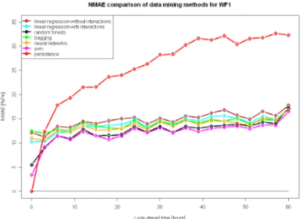
Figure 2: Comparison of NMAE results in the case of the wind farm WF1 situated on a com-plex terrain
Figure 3: Comparison of NMAE results in the case of the wind farm WF2 situated on a flat terrain
Figure 4: Comparison of NMAE results in the case of the wind farm WF3 situated on a flat terrain
Figure 5: Comparison of NRMSE results in the case of the wind farm WF1 situated on a com-plex terrain
Figure 6: Comparison of NRMSE results in the case of the wind farm WF2 situated on a flat terrain
Figure 7: Comparison of NRMSE results in the case of the wind farm WF3 situated on a flat terrain
observation as forecast for all horizons. Persis-tence is commonly used as a benchmark model in wind power forecasting.
The first common conclusion is that all models outperform persistence (excepted for 0-horizon which is a particular case corresponding to now-casting) and the level of accuracy depends of the terrain. Thus, we can observe a higher error level for WF1, which is situated on a complex terrain, compared to WF2 and WF3, which are on flat terrains. Then, for the three wind farms, we observe a global superiority of the non-linear models over the linear ones. This could be easily explained by the non-linear relationship between wind and power.
Even if the non-linear models presented here permit to improve the global performance when compared to linear ones, it should be noticed that the performances of the simple linear ap-proach is still reasonably good when compared to the persistence reference model. It should also be noticed that the results presented here are comparable to results found in the literature for wind farms located in similar terrains.
5
Conclusions
This paper presents a comparison of the perfor-mance of various data mining algorithms applied to short-term wind power forecasting. The inter-est of non-linear methods is illustrated for which the performance is equivalent to that found in the literature for wind farms located in simi-lar terrains. The comparison has revealed that Random Forest outperforms the rest of the mod-els. This model, originally applied here for wind power forecasting, is interesting since it does not require a long architecture optimisation step, only the number of trees in the forest has to be optimised.
Moreover, a generalization of Random Forests, Quantile Regression Forests give a non-parametric way of estimating conditional quantiles for high-dimensional predictor vari-ables [6, 5]. Thus provides an additional information on the uncertainty of the predic-tions for performing efficiently funcpredic-tions such as reserves estimation, unit commitment, trading in electricity markets, a.o. Such prediction (de-terministic with prediction intervals) is named probabilistic forecasting and are, nowadays, an important research field.
France for providing the data for the various case studies. This work was performed in the frame of project ENSEOLE, funded in part by ADEME, the French Environment and En-ergy Management Agency and a special thanks to Philippe Besse, professor at the engineering school INSAT.
References
[1] G. & Brownsword R. Giebel, G.; Karinio-takis. The state-of-the-art in short-term pre-diction of wind power - from a danish per-spective, 2003.
[2] S. Santoso, M. Negnevitsky, and N. Hatziar-gyriou. Data mining and analysis tech-niques in wind power system applications: abridged. Power Engineering Society Gen-eral Meeting, 2006. IEEE, pages 3 pp.–, 18-22 June 2006.
[3] Leo Breiman. Bagging predictors. Machine Learning, 24(2):123140, August 1996. [4] Charles J. Stone Leo Breiman, Jerome
Fried-man and R.A. Olshen.Classification and Re-gression Trees. Chapman & Hall/CRC, 1984. [5] Jeremie Juban, Lionel Fugon, and George Kariniotakis. Probabilistic short-term wind power forecasting based on kernel density estimators. In Proceedings of the European Wind Energy Conference, Milan, Italy, 7-10 May 2007.
[6] Nicolai Meinshausen. Quantile regression forests. Journal of Machine Learning Re-search, 7:983999, June 2006.