An Incremental On-line Classifier for Imbalanced, Incomplete, and Noisy Data

An Incremental On-line Classifier for Imbalanced,

Incomplete, and Noisy Data

Marko Tscherepanow

and

S¨oren Riechers

Abstract. Incremental on-line learning is a research topic gaining

increasing interest in the machine learning community. Such learning methods are highly adaptive, not restricted to distinct training and ap-plication phases, and applicable to large volumes of data. In this pa-per, we present a novel classifier based on the unsupervised topology-learning TopoART neural network. We demonstrate that this classi-fier is capable of fast incremental on-line learning and achieves excel-lent results on standard datasets. We further show that it can success-fully process imbalanced, incomplete, and noisy data. Due to these properties, we consider it a promising component for constructing artificial agents operating in real-world environments.

1

Introduction

The development of artificial agents with cognitive capabilities as they are found in humans and animals is still an unsolved problem. While biological agents can manage uncertain ever-changing envi-ronments with complex interdependencies, artificial agents are often limited to very specific, extremely simplified, and unchanging prob-lems.

One possibility to improve the performance of current artifi-cial systems is the usage of incremental learning mechanisms (e.g, [1], [18], and [19]). In contrast to traditional machine learning ap-proaches based on distinct training and application phases, incremen-tal approaches have to cope with additional difficulties – the most im-portant being thestability-plasticity dilemma[15]: while plasticity is required in order to learn anything new, stability ensures that already acquired knowledge does not get lost in an uncontrolled way.

Sensor data obtained in natural environments often exhibit charac-teristics which further impede learning. In particular, their distribu-tions can be non-stationary, noisy, and imbalanced. In addition, indi-vidual input vectors may be incomplete, for instance, due to different sensor latencies.

In this paper, we present an incremental classifier (see Section 4) based on the unsupervised TopoART neural network [26] (see Sec-tion 3). It is capable of stable and plastic incremental on-line learning and can cope with noisy, imbalanced, and incomplete data. These properties are shown using synthetic datasets (see Section 3) and real-world datasets from the UCI machine learning repository [12] (see Section 5).

2

Related Work

Adaptive Resonance Theory (ART) neural networks constitute an early approach to unsupervised incremental on-line learning. They

1 _{Applied Informatics, Bielefeld University, Germany, email:}

[email protected], [email protected]

incrementally learn a set of templates called categories. Some well-known ART variants are Fuzzy ART [5] and Gaussian ART [29]. While Fuzzy ART is capable of stable incremental learning using hyperrectangular categories but is prone to noise, the categories of Gaussian ART are Gaussians, which diminishes its sensitivity to noise but impairs the stability of learnt representations.

Regarding the formed representations, Gaussian ART is strongly related to on-line kernel density estimation (oKDE) [20]: oKDE in-crementally estimates a Gaussian mixture model representing a given data distribution. Depending on an adjustable parameter, the esti-mated distribution is stable to a certain degree.

Incremental topology-learning neural networks, such as Growing Neural Gas [13], constitute an alternative approach to unsupervised on-line learning. Some of these networks, e.g., the Self-Organising Incremental Neural Network (SOINN)[14] and Incremental Grow-ing Neural Gas (IGNG) [21], alleviate the problems resultGrow-ing from the stability-plasticity dilemma. However, they rely on neurons rep-resenting prototype vectors. During learning, any shift of these pro-totype vectors in the input space inevitably causes some loss of in-formation.

TopoART [26] has been proposed as a neural network combining properties from ART and topology-learning neural networks. As its architecture and representations are based on Fuzzy ART [5], each neuron (also called node) represents a hyperrectangular region of the input space, which can only grow during learning. As a result, once an input vector has been enclosed by a category, it will stay inside. In addition, TopoART inherited the insensitivity to noise from SOINN [14], which is a major improvement in comparison to Fuzzy ART.

The approaches mentioned above are not applicable to supervised learning tasks such as classification. However several extensions ex-ist that enable their application to such problems, e.g., ARTMAP [4] for ART networks, Bayes’ decision rule [28] for mixture models, and Life-long Learning Cell Structures [16] for prototype-based in-cremental topology-learning neural networks. The resulting super-vised learning methods usually inherit the characteristics of their unsupervised components and ancestors, respectively. In particular, they learn locally; i.e., adaptations are restricted to a limited set of parameters.

The Perceptron [22], a very early approach to supervised on-line learning, possesses a distributed memory. As a consequence, all trainable parameters are altered during learning rendering Percep-trons prone to catastrophic forgetting. Furthermore, they have a fixed structure limiting the complexity of the knowledge that can be stored. These problems were inherited by multi-layer Perceptrons (MLPs) [23]. Cascade-Correlation neural networks [11] partially solve them by means of an incremental structure. But they are restricted to off-line (batch) learning.

b

a

F2

F0

F1

F2

F1

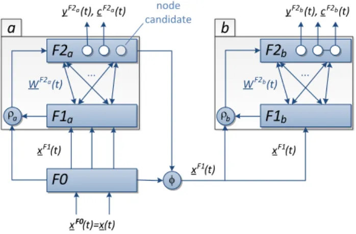
Figure 1. TopoART neural networks consist of two modules sharing the

input layerF0. Both modules function in an identical way. However, input to modulebis controlled by modulea.

Support vector machines (SVMs) [8], an alternative extension of Perceptrons, learn by solving a quadratic programming problem based on a fixed training set; i.e., off-line. A subset of the training samples, called support vectors, is chosen to construct separating hy-perplanes. Although there are approaches to on-line SVMs (e.g., [2] and [6]), the underlying model imposes several problems: an ade-quate kernel has to be selected in advance, the number of occurring classes needs to be known or is limited to two, and a possibly large set of input samples has to be collected in addition to the support vectors to stabilise the learning process.

Recently, several incremental classification frameworks based on ensemble learning, e.g, ADAIN [17] and Learn++.NSE [10], have been proposed. These approaches assume that data be provided in data chunks containing multiple samples. As for each of these chunks an individual base classifier is trained, a voting mechanism is re-quired so as to obtain a common prediction. Furthermore, additional learning methods may be necessary; ADAIN, for instance, uses an MLP to construct a mapping function connecting past experience with present data.

TopoART-C, the classifier presented in this paper, is based on the unsupervised TopoART network. TopoART was chosen as a ba-sis in order to take advantage of its beneficial properties, namely its capability of stable incremental on-line learning of noisy data. TopoART-C constitutes an extension of TopoART for classification tasks like the Simplified Fuzzy ARTMAP approach [27] used for Fuzzy ART. The usage of an additional mask layer further allows predictions to be made based on incomplete data.

3

TopoART

TopoART is strongly related to Fuzzy ART [5]: it shares its basic rep-resentations, its choice and match functions, and its principal search and learning mechanisms. However, TopoART extends Fuzzy ART in such a way that it becomes insensitive to noise and capable of top-ology learning. One important part of the noise filtering mechanism is the combination of multiple Fuzzy ART-like modules, where pre-ceding modules filter the input for successive ones. Therefore, the standard TopoART architecture as proposed in [26] (see Fig. 1) con-sists of two modules (a & b). Besides noise filtering, these modules cluster input data at two different levels of detail.

The clusters are composed of hyperrectangular categories, which

are encoded in the weights of neurons in the respectiveF2layer. By learning edges between different categories, clusters of arbitrary shapes are formed.

If an input vector

x(t) =

x1(t), . . . , xd(t) T

(1) is fed into such a network, complement coding is performed resulting in the vector

xF1(t) =

x1(t), . . . , xd(t),1−x1(t), . . . ,1−xd(t)

T

. (2)

As a consequence of this encoding that was inherited from Fuzzy ART, all elementsxi(t)of the input vectorx(t)must be normalised to the interval[0,1].2

xF1(t)is first propagated to theF1layer of modulea. From here, it is used to activate theF2nodes of moduleabased on their weights given by the matrixWF2a_(t).

As TopoART networks learn incrementally and on-line, training and prediction steps can be mixed arbitrarily. During training, the activation (choice function)

zjF2(t) = xF1(t)∧wF_j2(t) 1 α+ wF_j2(t) 1 (3) of eachF2nodejis computed first.k·k1and∧denote the city block

norm and a component-wise minimum operation, respectively (cf. [5]). The node with the highest activation becomes the best-matching nodebm. Its weights are adapted if the match function

xF1(t)∧wF_j2(t) 1 xF1(t) 1 ≥ρ (4)

is fulfilled forj=bm. Otherwise, the current nodebmis reset and a new best-matching node is determined. If a suitable best-matching nodebmhas been found, a second-best-matching nodesbmfulfilling Eq. 4 is sought.

The categories of the best-matching node and the second-best-matching node are allowed to grow in order to enclosexF1_(t)or

partially learnxF1(t), respectively:

wF_bm2(t+ 1) = xF1(t)∧wF_bm2(t) (5) wFsbm2 (t+ 1) = βsbm xF1(t)∧wFsbm2 (t) +(1−βsbm)w F2 sbm(t) (6)

In order to learn the topology of the data,bmandsbmare con-nected by an edge. Already existing edges are not modified. If the

F2layer is empty or no node is allowed to learn, a new node with

wF2a

new(t+ 1)=x

F1_{(t)is incorporated.}

According to Eq. 4, the maximum size of the categories is limited by the vigilance parameterρ. Here, the vigilance parameterρb of modulebis determined depending on the vigilance parameterρaof modulea:

ρb= 1

2(ρa+ 1) (7)

A value ofρa=0means that a single category of moduleacan cover the entire input space, while a value ofρa=1results in categories containing single samples.

2_{This normalisation usually requires an estimation of the minimum and}

0 0.2 0.4 0.6 0.8 1 0 0.2 0.4 0.6 0.8 1

input data, training phase 1

0 0.2 0.4 0.6 0.8 1 0 0.2 0.4 0.6 0.8 1

input data, training phase 2

0 0.2 0.4 0.6 0.8 1 0 0.2 0.4 0.6 0.8 1

input data, training phase 3

0 0.2 0.4 0.6 0.8 1 0 0.2 0.4 0.6 0.8 1 TA b: ρb=0.96, βsbm=0.37, φ=6, τ=200 0 0.2 0.4 0.6 0.8 1 0 0.2 0.4 0.6 0.8 1 TA b: ρb=0.96, βsbm=0.37, φ=6, τ=200 0 0.2 0.4 0.6 0.8 1 0 0.2 0.4 0.6 0.8 1 TA b: ρb=0.96, βsbm=0.37, φ=6, τ=200

Figure 3. Results for non-stationary data. The training was performed in

three successive phases (top row). In the bottom row, the corresponding clusters formed by a TopoART network after finishing the respective phase

are shown. The network parameters were adopted from Fig. 2.

TheF2neurons of both modules possess a counter denoted by

nj. Each time a node is adapted, the corresponding counter is incre-mented. Furthermore, allF2nodesjwithnj<φare removed every

τ learning cycles of the respective module. Therefore, such neurons are called node candidates. In contrast, nodes withnj≥φare perma-nent; i.e., their categories are completely stable. The node candidates and the permanent nodes can be considered as the short-term mem-ory and the long-term memmem-ory of the network, respectively.

xF1_(t)

is only propagated to module bfor training if the best-matching node of moduleais permanent. In moduleb, the processes of category search and weight adaptation are repeated for the corres-pondingF2nodes usingρbinstead ofρa. In conjunction with the input filtering and the node-removal process, this constitutes a pow-erful noise reduction mechanism. Figure 2 illustrates this mechanism in comparison to two other popular unsupervised learning methods. The applied dataset consists of six clusters with 15,000 samples each as well as ten percent of uniformly distributed random noise (100,000 samples in total). In order to create a stationary data distribution, the samples were presented once in random order.

TopoART and SOINN were able to determine a detailed clustering reflecting the six clusters of the input distribution in a high level of detail. Here, the representation was refined from moduleato mod-uleband from SOINN layer 1 (SOINN 1) to SOINN layer 2 (SOINN 2). The representation of oKDE also reflects the underlying compo-nents, but does not include the topological structures. Furthermore, several Gaussians exclusively represent noise regions.

The capability of TopoART to incrementally learn stable repre-sentations from noisy non-stationary data is demonstrated in Fig. 3. Here, the input data used before were reordered and presented in three consecutive phases. After each training phase, TopoART has learnt the respective new clusters and the clusters formed during ear-lier training phases remained stable.

For prediction, xF1(t) is directly propagated to both modules where the respective best-matching nodes are determined. Here, usu-ally the alternative activation function

zFj2(t) = 1− xF1(t)∧wF_j2(t) −wFj2(t) 1 d (8)

that is independent from the category size is applied and the match

function is not computed. The output of a module consists of a vector

yF2(t)with

yFj2(t) =

0 ifj6=bm

1 ifj=bm (9)

and a vectorcF2(t)reflecting the clustering structure. For reasons of stability, node candidates are ignored during prediction.

Details on the adjustment and the effects of the parametersρa,

βsbm,φ, andτcan be found in [26].

4

TopoART-C

In contrast to TopoART, which clusters presented data, a classifier requires additional information. In particular, a class labelλiis asso-ciated with each input vectorx(t)comprising one or more features

xi(t). This label is either presented for training or predicted based onx(t).Λ(t)denotes the set of all known class labels at time stept. In incremental learning scenariosΛ(t)may grow if new data become available. The current number of known classes is given by|Λ(t)|. In order to construct a classifier inheriting the advantageous properties of TopoART, the principal structure of TopoART was preserved and extended by three additional layers (see Fig. 4).

Both modules obtained a classification layer F3, the nodes of which represent possible classesλi. These layers receive the out-putyF2_(t)

of the respective F2 layer as input. Furthermore, a mask layerF0m was incorporated so as to enable predictions based on incomplete input data.

4.1

Training

TopoART-C is trained in a similar way to TopoART. But in order to account for the class labels, the match function (cf. Eq. 4) was modified: xF1(t)∧wF_j2(t) 1 xF1(t) 1 ≥ρ and class(j) =λ(t) (10)

b

a

F2

F0

F1

F2

F1

F3

F0

F3

Figure 4. Structure of TopoART-C. TopoART-C extends the structure of

TopoART by adding a classification layerF3to each module and a mask layerF0mto moduleb.

0 0.2 0.4 0.6 0.8 1 0 0.2 0.4 0.6 0.8 1 input data 1 2 3 4 5 6 0 0.2 0.4 0.6 0.8 1 0 0.2 0.4 0.6 0.8 1 TA a: ρ a=0.92, βsbm=0.37, φ=6, τ=200 0 0.2 0.4 0.6 0.8 1 0 0.2 0.4 0.6 0.8 1 TA b: ρ b=0.96, βsbm=0.37, φ=6, τ=200 0 0.2 0.4 0.6 0.8 1 0 0.2 0.4 0.6 0.8 1 SOINN 1: λ1=250, age1=250, c1=0.5 0 0.2 0.4 0.6 0.8 1 0 0.2 0.4 0.6 0.8 1 SOINN 2: λ 2=250, age2=50, c2=0.05 0 0.2 0.4 0.6 0.8 1 0 0.2 0.4 0.6 0.8 1 oKDE: D th=0.01, f=1, Ninit=10 a b c d e f

Figure 2. Clustering results for stationary data. A two-dimensional synthetic data distribution was learnt by TopoART (TA), SOINN, and oKDE. The relevant

parameters were manually chosen in such a way as to fit the data. Different clusters of TopoART (b & c) and SOINN (d & e) are coloured differently. For SOINN, the edges connecting individual prototype vectors are shown, as well. In contrast to TopoART and SOINN, the distribution estimated by oKDE (f)

consists of a mixture of Gaussians drawn as ellipses marking the standard deviations. It does not reflect the topological structure of the data.

Here,λ(t)denotes the class label ofx(t)andclass(j)the class en-coded by theF3node that is connected with nodej.3

Assuming the match function cannot be fulfilled for any existing

F2node, a new one withwF2

new(t+ 1)=x F1_(t)

is incorporated like in the original TopoART network. Additionally, it is linked to theF3 node representingλ(t). If the network does not knowλ(t), a newF3 node representing this label is inserted.

4.2

Prediction

During prediction, the class labelλiwhich best fits the input vector

x(t)is computed by modulebusing the decision rule:

e(t) = arg max λi∈Λ(t)

dλi(t) (11)

The discrimination functiondλi(t)measures the similarity ofx(t)

with the internal representation of classλi:

dλi(t) = X j∈Υb(t) class(j)=λi yF2b j (t) (12)

dλi(t)depends on the output y

F2b _{of theF2layer of module b.}

The set of all nodes of this layer is denoted byΥb(t). Moduleais completely neglected, as it is only required for training in order to filter irrelevant data.

If the original output function (Eq. 9) is applied,e(t)yields the class label of the permanent node whose category has the closest distance tox(t). But depending on the class boundaries, the resulting prediction may be suboptimal. Therefore, we propose a more general output function, which can consider more than one node and allows for problem specific adaptations. Here, two principal cases have to be distinguished: eitherx(t)lies inside one or more categories or it is enclosed by no category. In the first case, the class label can be derived from the enclosing categories summarised in the set

E(t) =

j∈Υb(t) :zjF2b(t) = 1 . (13)

These nodes are characterised by a maximum activationzF2b

j (t) ac-cording to Eq. 8. Using the modified output function

yF2b j (t) = ( 1 , ifj= arg min k∈E(t)Sk(t) 0 , otherwise, (14)

3_{EachF2node can only be connected with a singleF3node.}

the prediction corresponds to the class label associated with the smallest category containingx(t). The category sizeSk(t)is defined as Sk(t) = d X i=1 1−w F2 k,d+i(t) −wFk,i2(t) . (15)

In the second case, i.e., if no category enclosesx(t), predictions are computed based on the setNof closest neighbours:

N(t) =

j∈Υb(t) :zjF2b(t)≥µ+ 1.28σ (16)

µandσdenote the arithmetic mean and the standard deviation of

zF2b

j (t)over allF2b neurons, respectively. If the activations were normally distributed,N(t) would only contain those 10% of the neurons that have the highest activations.

The contribution of each neighbour to the output function is in-versely proportional to the distance between its category andx(t):

yF2b j (t) =          1 1−zF_j2b(t) P n∈N(t) 1 1−zF2b n (t) , ifj∈ N(t) 0 , otherwise (17)

Depending on the data distribution and for computational reasons it may be advantageous to further limit the number of considered nodes. Therefore, we incorporated an additional parameterνwhich denotes the maximum cardinality ofE(t)andN(t). It does not affect the underlying representations and may be changed during the appli-cation of the network. To obtain repeatable results, elements need to be added to both sets in a predefined way (cf. Eqs. 13 and 16). There-fore, we decided to add nodes in increasing order of their indices to

E(t)and in decreasing order of their activations toN(t). Provided that the cardinality has reached the value ofν, the insertion of new elements is stopped. As a result, established and certain knowledge is preferred over recently acquired and uncertain knowledge. Due to this difference to the original output function (cf. Eq. 9), which treats all nodes equally, we decided to consider not only permanent nodes but also node candidates for prediction. As a result, the predictions become slightly less stable. However, the network is better adapted to recent input, in particular if no established knowledge is available. In order to make predictions based on incomplete input vectors, the mask layerF0mis used. Its neurons, the output of which is given by the mask vector

mF0(t) = mF10(t), . . . , m F0 d (t) T , (18)

inhibit the network connections that encode elements of the input vector that are not available; i.e., presented elements are charac-terised by a mask valuemF0

i (t)of0and unknown elements by a value of1. Hence, the indices of the relevant elements ofxF1(t)(cf. Eq. 2) are given by the index set

M0 =

i, i+d:mFi0(t) = 0 . (19) UsingM0

, the activation of theF2nodes of modulebcan be determined solely based on the non-inhibited F1 neurons:

zF2b j (t) = 1− P i∈M0 min x F1 i (t), w F2b ji (t) −wF2b ji (t) 1 2|M 0_| (20)

If required, the maximum activation over allF2nodes of moduleb

can be applied as a measure of the degree of knowledge the network has about a certain input vector. Then, input vectors can be rejected as unknown if the maximum activation is below a threshold.

5

Results

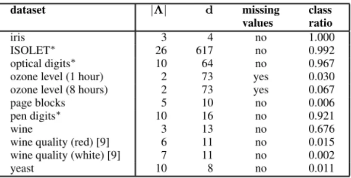
We evaluated TopoART-C using several real-world datasets from the UCI machine learning repository [12]. In order to show the beneficial properties of TopoART-C, we selected datasets with varying numbers of classes and features, with and without missing values, and with balanced and imbalanced classes (see Table 1). Here, the class ratio denotes the ratio between the number of samples contained in the smallest class and in the largest class, respectively. Thus, a class ratio of1shows that a dataset is completely balanced, while class ratios close to0indicate imbalanced datasets.

dataset |Λ| d missing class

values ratio

iris 3 4 no 1.000

ISOLET∗ 26 617 no 0.992

optical digits∗ _{10 64 no 0.967}

ozone level (1 hour) 2 73 yes 0.030

ozone level (8 hours) 2 73 yes 0.067

page blocks 5 10 no 0.006

pen digits∗ 10 16 no 0.921

wine 3 13 no 0.676

wine quality (red) [9] 6 11 no 0.015

wine quality (white) [9] 7 11 no 0.002

yeast 10 8 no 0.011

Table 1. Number of classes|Λ|, number of featuresd, existence of missing values and class ratio for the considered datasets. Those datasets marked

with∗contain an independent test set.

For comparison, we used several well-known on-line and off-line classifiers: the k-nearest neighbour classifier3 (kNN), the na¨ıve Bayes classifier3 _{(NB), random trees}3 _{(RTs), the Simplified Fuzzy}

ARTMAP (SFAM) [27], and support vector machines4 (SVMs) using different kernels. These classifiers were compared based on the harmonic mean accuracy

ACChm= |Λ| P λi∈Λ 1 ACC(λi) (21) 3_{implemented in OpenCV v2.2 [3]} 4_{implemented in LIBSVM v3.11 [7]}

as proposed in [25] for imbalanced datasets. Here,ACC(λi) de-notes the fraction of correctly classified samples of classλi. In con-trast to the total accuracy5 and the arithmetic mean of the class-specific accuraciesACC(λi),ACChmprevents large correctly

clas-sified classes from dominating the classification results; e.g., if one class cannot be recognised at all,ACChmdrops to zero, independent

of the number of test samples available for this class. Provided that the classification problem is entirely balanced and the class-specific accuracies are equal, all three accuracy measures are equal.

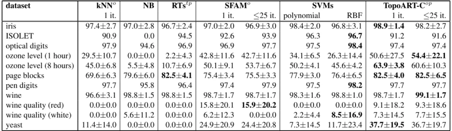
Table 2 shows the classification results. These results were either obtained using five-fold cross-validation or refer to the independent test set that has neither been used for training nor the optimisation of model parameters before, if available (cf. Table 1). The relevant par-ameters of the classifiers were determined by means of grid search.6

For training, all features were normalised to the interval[0.05,0.95]. Input vectors containing missing values were ignored (training and prediction) and counted as errors (prediction) if the respective clas-sifier was not able to process incomplete data.

TopoART-C achieved excellent results for the majority (6of11) of the datasets. In particular, it outperformed the other classifiers on4of6imbalanced7 _{datasets including those with missing values}

and reached comparatively high accuracies for the remaining two datasets ‘wine quality (red)’ and ‘wine quality (white)’. Regarding balanced data, SVMs performed better, especially on the ‘ISOLET’ dataset, which is most likely caused by its large number of features. Nevertheless, TopoART-C achieved the maximum accuracy on2of 5balanced datasets. In addition, TopoART-C often reached very high accuracies after a single presentation of all training samples, which is a good benchmark for incremental on-line learning; without the ca-pability of stable incremental learning, an on-line learning approach such as TopoART (cf. Eqs. 5 and 6) would be prone to catastrophic forgetting resulting in worse results.

6

Conclusion and Outlook

We presented the novel incremental classifier TopoART-C that is capable of fast on-line learning (cf. Table 2). Accurate predictions can even be made if the input vectors contain missing values. As TopoART-C contains the unsupervised TopoART network as major learning component, it is insensitive to noise (cf. Fig. 2) and can be applied to non-stationary data (cf. Fig. 3). These properties of TopoART-C make it an excellent choice for the application to real-world on-line learning tasks, as they occur, for instance, in cognitive robotics. In addition, the clusters learnt by the TopoART subnet could provide additional information on the underlying data.

Furthermore, TopoART-C is not restricted to the usage of TopoART; alternative neural networks with a TopoART-like structure such as Hypersphere TopoART [24] can be applied as well. Since Hypersphere TopoART does not perform complement coding, the re-sulting classifier could process arbitrarily scaled values even if their range is not completely known in advance.

5_{overall ratio of correctly classified samples}

6_{kNN:k∈ {1,2, . . . ,25};RTs:use surrogates∈ {false,true},}

variableImportance ∈ {false,true}, nactive vars = dx_{withx∈[0.1,0.9]and step size0.1;SFAM:ρ∈[0.75,1]with step} size0.01,β ∈ [0.2,1]with step size0.2;SVMs:C = 10x_{withx ∈} [−4,4]and step size0.5,γ = 10x_{withx ∈ [−4,4]and step size0.5} (RBF kernel),coef0= 10xwithx∈[−4,4]and step size0.5 (polyno-mial kernel), degree∈ {1,2,3,4,5}(polynomial kernel);TopoART-C: ρa ∈ [0.75,1]with step size0.01,βsbm ∈ [0,1]with step size0.2, φ∈ {1,2,3,4,5},ν∈ {1,2, . . . ,25}

dataset kNNo NB RTstp SFAMo SVMs TopoART-Cop

1 it. 1 it. ≤25 it. polynomial RBF 1 it. ≤25 it.

iris 97.4±2.7 97.0±2.8 96.7±2.4 97.0±2.0 96.9±3.0 98.4±2.0 96.8±3.1 98.9±1.4 98.2±2.7

ISOLET 90.9 0.0 94.5 92.6 93.9 96.3 96.7 91.2 91.6

optical digits 97.9 94.6 96.9 96.9 97.7 97.5 98.4 97.4 97.4

ozone level (1 hour) 29.5±10.7 0.0±0.0 2.2±4.3 42.8±11.6 42.7±11.6 34.1±6.5 26.3±14.4 50.6±27.5 54.4±22.1

ozone level (8 hours) 45.0±6.8 5.5±4.8 10.7±6.9 50.1±9.1 53.7±6.7 50.2±4.1 45.6±4.2 63.9±3.8 60.6±10.3 page blocks 69.6±6.3 79.6±6.0 82.5±4.1 75.4±3.4 75.5±3.3 77.9±3.0 76.4±6.5 82.5±4.0 82.5±6.5

pen digits 97.7 95.8 96.4 97.4 97.9 97.5 98.2 97.7 97.7

wine 96.6±3.1 98.8±1.5 98.8±1.5 98.7±1.7 98.7±1.7 98.3±1.6 98.8±1.0 98.7±1.7 99.1±1.7

wine quality (red) 0.0±0.0 0.0±0.0 0.0±0.0 15.8±20.1 15.9±20.2 0.0±0.0 0.0±0.0 9.1±18.2 9.3±18.6 wine quality (white) 0.0±0.0 5.6±11.2 0.0±0.0 6.2±12.3 0.0±0.0 2.2±4.4 8.5±16.9 7.3±14.5 7.7±15.5 yeast 11.4±14.0 0.0±0.0 0.0±0.0 24.9±20.9 24.4±20.8 7.3±14.5 11.7±23.4 37.7±19.5 36.7±19.7

Table 2. Harmonic mean accuracies and their standard deviations (over the cross-validation runs) in percent. The best results for each dataset are highlighted.

In order to alleviate the comparison, some relevant capabilities of the classifiers are indicated by superscripts:o=on-line learning,t=accept missing values for training, andp=accept missing values for prediction. In order to compensate for the negative effects of a possibly too small number of training steps, the

respective training sets were presented to the on-line learning approaches except for the kNN classifier up to 25 times. The results are given for the first iteration (1 it.) and when they converged or the maximum number of iterations was reached (≤25 it.).

ACKNOWLEDGEMENTS

This work was partially funded by the German Research Foundation (DFG), Excellence Cluster 277 “Cognitive Interaction Technology”.

REFERENCES

[1] Elmar Bergh¨ofer, Denis Schulze, Marko Tscherepanow, and Sven Wachsmuth, ‘ART-based fusion of multi-modal information for mobile robots’, inProceedings of the International Conference on Engineering Applications of Neural Networks, volume 363 ofIFIP AICT, pp. 1–10, Corfu, Greece, (2011). Springer.

[2] Antoine Bordes, Seyda Ertekin, Jason Weston, and L´eon Bottou, ‘Fast kernel classifiers with online and active learning’,Journal of Machine Learning Research,6, 1579–1619, (2005).

[3] Gary Bradski and Adrian Kaehler,Learning OpenCV: Computer Vision with the OpenCV Library, O’Reilly, 2008.

[4] Gail A. Carpenter, Stephen Grossberg, and John H. Reynolds, ‘ARTMAP: Supervised real-time learning and classification of nonsta-tionary data by a self-organizing neural network’,Neural Networks,4, 565–588, (1991).

[5] Gail A. Carpenter, Stephen Grossberg, and David B. Rosen, ‘Fuzzy ART: Fast stable learning and categorization of analog patterns by an adaptive resonance system’,Neural Networks,4, 759–771, (1991). [6] Gert Cauwenberghs and Tomaso Poggio, ‘Incremental and

decremen-tal support vector machine learning’, inNeural Information Processing Systems, pp. 409–415, (2000).

[7] Chih-Chung Chang and Chih-Jen Lin, ‘LIBSVM: A library for sup-port vector machines’,ACM Transactions on Intelligent Systems and Technology,2(3), 27:1–27:27, (2011). Software available athttp: //www.csie.ntu.edu.tw/˜cjlin/libsvm.

[8] Corinna Cortes and Vladimir Vapnik, ‘Support-vector networks’, Ma-chine Learning,20, 273–297, (1995).

[9] Paulo Cortez, Ant´onio Cerdeira, Fernando Almeida, Telmo Matos, and Jos´e Reis, ‘Modeling wine preferences by data mining from physic-ochemical properties’, Decision Support Systems, 47(4), 547–553, (2009).

[10] Ryan Elwell and Robi Polikar, ‘Incremental learning of concept drift in nonstationary environments’,IEEE Transactions on Neural Networks,

22(10), 1517–1531, (2011).

[11] Scott E. Fahlman and Christian Lebiere, ‘The cascade-correlation learn-ing architecture’, inNeural Information Processing Systems, pp. 524– 532, (1989).

[12] A. Frank and A. Asuncion. UCI machine learning repository, 2010. [13] Bernd Fritzke, ‘A growing neural gas network learns topologies’, in

Neural Information Processing Systems, pp. 625–632, (1994). [14] Shen Furao and Osamu Hasegawa, ‘An incremental network for on-line

unsupervised classification and topology learning’,Neural Networks,

19, 90–106, (2006).

[15] Stephen Grossberg, ‘Competitive learning: From interactive activation to adaptive resonance’,Cognitive Science,11, 23–63, (1987). [16] Fred H. Hamker, ‘Life-long learning cell structures—continuously

learning without catastrophic interference’,Neural Networks,14, 551– 573, (2001).

[17] Haibo He, Sheng Chen, Kang Li, and Xin Xu, ‘Incremental learning from stream data’,IEEE Transactions on Neural Networks,22(12), 1901–1914, (2011).

[18] Marc Kammer, Marko Tscherepanow, Thomas Schack, and Yukie Na-gai, ‘A perceptual memory system for affordance learning in humanoid robots’, in Proceedings of the International Conference on Artifi-cial Neural Networks, volume 6792 ofLNCS, pp. 349–356. Springer, (2011).

[19] Stephan Kirstein and Heiko Wersing, ‘A biologically inspired approach for interactive learning of categories’, inProceedings of the Inter-national Conference on Development and Learning, pp. 1–6. IEEE, (2011).

[20] Matej Kristan, Aleˇs Leonardis, and Danijel Skoˇcaj, ‘Multivariate online kernel density estimation with Gaussian kernels’,Pattern Recognition,

44(10–11), 2630–2642, (2011).

[21] Yann Prudent and Abdellatif Ennaji, ‘An incremental growing neural gas learns topologies’, inProceedings of the International Joint Con-ference on Neural Networks, volume 2, pp. 1211–1216. IEEE, (2005). [22] Frank Rosenblatt, ‘The perceptron: A probabilistic model for

infor-mation storage and organization in the brain’,Psychological Review,

65(6), 386–408, (1958).

[23] David E. Rumelhart, Geoffrey E. Hinton, and Ronald J. Williams, ‘Learning internal representations by error propagation’, inParallel Distributed Processing – Explorations in the Microstructure of Cog-nition, volume 1, 318–362, MIT Press, seventh edn., (1988).

[24] Marko Tscherepanow, ‘Incremental on-line clustering with a topology-learning hierarchical ART neural network using hyperspherical cat-egories’, inPoster and Industry Proceedings of the Industrial Confer-ence on Data Mining, pp. 22–34. ibai-publishing, (2012).

[25] Marko Tscherepanow, Nickels Jensen, and Franz Kummert, ‘An incre-mental approach to automated protein localisation’,BMC Bioinformat-ics,9(445), (2008).

[26] Marko Tscherepanow, Marko Kortkamp, and Marc Kammer, ‘A hierar-chical ART network for the stable incremental learning of topological structures and associations from noisy data’,Neural Networks,24(8), 906–916, (2011).

[27] Mohammad-Taghi Vakil-Baghmisheh and Nikola Paveˇsi´c, ‘A fast sim-plified fuzzy ARTMAP network’,Neural Processing Letters,17(3), 273–316, (2003).

[28] Andrew R. Webb and Keith D. Copsey,Statistical Pattern Recognition, Wiley, third edn., 2011.

[29] James R. Williamson, ‘Gaussian ARTMAP: a neural network for fast incremental learning of noisy multidimensional maps’,Neural Net-works,9(5), 881–897, (1996).