Event Detection from Text Data

Bachelor thesis

Event Detection from Text Data

Tom´

aˇ

s Kala

Supervisor: doc. Ing. Jiˇr´ı Kl´ema, PhD.

Department of Cybernetics

Faculty of Electrical Engineering

Czech Technical University in Prague

Czech Technical University in Prague Faculty of Electrical Engineering

Department of Cybernetics

BACHELOR PROJECT ASSIGNMENT

Student: Tomáš K a l a

Study programme: Open Informatics

Specialisation: Computer and Information Science

Title of Bachelor Project: Event Detection from Text Data

Guidelines:

1. Get familiar with the topic of event detection from potentially large text collections. 2. Reimplement the method of He et al. in Python and test it on a dataset provided by the thesis supervisor.

3. Propose and implement modifications of this algorithm. Consider changes in the cost function, utilization of document clustering with consequent topic dependent event detection and application of word/document embedding.

4. Extend the algorithm to be able to annotate the individual events and organize them. 5. Compare the results reached in the previous steps. Employ the list of real events given by the thesis supervisor to make the comparison as objective as possible.

Bibliography/Sources:

[1] He, Qi, Kuiyu Chang, and Ee-Peng Lim. "Analyzing feature trajectories for event detection."

Proceedings of the 30th annual international ACM SIGIR conference on Research and development in information retrieval. ACM, 2007.

[2] Fung, Gabriel Pui Cheong, et al. "Parameter free bursty events detection in text streams."

Proceedings of the 31st international conference on Very large data bases. VLDB Endowment, 2005. [3] Mikolov, Tomas, Chen, Kai, Corrado, Greg, and Dean, Jeffrey. "Efficient Estimation of Word

Representations in Vector Space". In Proceedings of Workshop at ICLR, 2013.

[4] Zhong, Shi. "Efficient online spherical k-means clustering." In Proceedings of the IEEE International Joint Conference on Neural Networks, 2005., vol. 5, pp. 3180-3185, 2005.

[5] Atefeh, Farzindar, and Wael Khreich. "A survey of techniques for event detection in twitter." Computational Intelligence 31.1, pp. 132-164, 2015.

Bachelor Project Supervisor: doc. Ing. Jiří Kléma, Ph.D.

Valid until: the end of the summer semester of academic year 2017/2018

L.S.

prof. Dr. Ing. Jan Kybic Head of Department

prof. Ing. Pavel Ripka, CSc. Dean

Author statement for

undergraduate thesis:

I declare that the presented work was developed independently and that I have listed all sources of information used within it in accordance with the methodical instruc-tions for observing the ethical principles in the preparation of university theses.

Prague, date ... ...

Abstract

Event detection is a process of analysis of text documents aiming to uncover real events happening in the world. It is based on the assumption that words appearing in similar documents and time windows are likely to concern the same real-world event. Therefore, our method attempts to group together words with similar tem-poral and semantic characteristics while discarding noisy words, not contributing to anything of interest. This results in a concise event representation through a set of representative keywords. These are then used to query the document collection to retrieve the actual event-related documents. Finally, we extract short summaries from these documents and annotate the events in a human-readable fashion. The keyword retrieval phase of our method is based on an existing event detection sys-tem, which we modify by employing a word embedding model to measure semantic similarity. The method is evaluated on a collection of 2 million documents from Czech news over a 13 months period and compared to the original method, not depending on word embeddings.

Keywords: Document retrieval, event detection, multi-document summarization, word embedding.

Abstrakt

Detekce ud´alost´ı je proces anal´yzy textov´ych dokument˚u za ´uˇcelem odhalen´ı ud´alost´ı, kter´e se bˇehem doby jejich vyd´an´ı staly ve svˇetˇe. Tento proces je zaloˇzen na pˇredpokladu, ˇze s´emanticky podobn´a slova se zv´yˇsen´ym v´yskytem bˇehem stejn´eho obdob´ı se pravdˇepodobnˇe vztahuj´ı ke stejn´e ud´alosti. N´ami zkouman´a metoda se tedy snaˇz´ı shlukovat dohromady slova s podobnou ˇcasovou nebo s´emantickou charakteristikou, a z´aroveˇn ignorovat slova nenesouc´ı ˇz´adnou informaci. To vede k jednoduch´e reprezentaci ud´alost´ı pomoc´ı skupin kl´ıˇcov´ych slov. Tato kl´ıˇcov´a slova jsou n´aslednˇe pouˇzita k dotazu do zkouman´e kolekce a z´ısk´an´ı dokument˚u vztahuj´ıc´ıch se k jednotliv´ym ud´alostem. Z tˇechto dokument˚u jsou nakonec extra-hov´ana kr´atk´a shrnut´ı pro bohatˇs´ı popis ud´alost´ı. F´aze z´ısk´av´an´ı kl´ıˇcov´ych slov je zaloˇzena na existuj´ıc´ım postupu, kter´y modifikujeme pouˇzit´ım modelu vnoˇrov´an´ı slov (word embedding) k mˇeˇren´ı s´emantick´e podobnosti. Metoda je vyhodnocena na kolekci 2 milion˚u dokument˚u z ˇcesk´ych novinov´ych server˚u vydan´e za obdob´ı 13 mˇes´ıc˚u, a porovn´ana s p˚uvodn´ım postupem nevyˇzaduj´ıc´ım vnoˇrov´an´ı slov.

Kl´ıˇcov´a slova: Z´ısk´av´an´ı dokument˚u, detekce ud´alost´ı, sumarizace v´ıce doku-ment˚u, word embedding.

Contents

3 Document stream and preprocessing 11 3.1 Preprocessing . . . 12

3.2 Word embeddings . . . 12

3.3 Document collection . . . 12

3.4 Document stream formally . . . 13

4 Word-level analysis 14 4.1 Binary bag of words model . . . 15

4.2 Computing word trajectories . . . 16

4.3 Spectral analysis . . . 17

5 Event detection algorithms 19 5.1 Original method . . . 19

5.1.1 Trajectory distance . . . 20

5.1.2 Document overlap . . . 20

5.1.3 Cost function . . . 20

5.1.4 Event detection algorithm . . . 20

5.2 Embedded greedy approach . . . 22

5.2.1 Semantic similarity . . . 22 5.2.2 Cost function . . . 23 5.3 Cluster-based approach . . . 23 5.3.1 Noise filtering . . . 24 5.3.2 Distance function . . . 25 5.3.3 Event detection . . . 26 6 Document retrieval 27 6.1 Event burst detection . . . 27

6.1.1 Event trajectory construction . . . 28

6.1.2 Trajectory filtering . . . 28

6.1.3 Event periodicity . . . 28

6.1.5 Burst detection . . . 30 6.2 Document retrieval . . . 31 7 Event annotation 33 7.1 Multi-document summarization . . . 34 7.2 Coverage function . . . 35 7.2.1 TFIDF similarity . . . 35 7.2.2 Word2Vec similarity . . . 36 7.2.3 TR similarity . . . 36 7.2.4 Keyword similarity . . . 36 7.3 Diversity function . . . 37 7.4 Optimization . . . 37 7.5 Results . . . 37 8 Evaluation 39 8.1 Precision, Recall, F-measure . . . 39

8.2 Redundancy . . . 41

8.3 Noisiness . . . 42

8.4 Purity . . . 43

8.5 Computation time . . . 45

9 Conclusion and future work 46 Bibliography 48 A Real events used for evaluation 52 B Annotated events 56 B.1 Original method . . . 56

B.2 Embedded-greedy method . . . 58

B.3 Cluster-based method . . . 59

Chapter 1

Introduction

As the number of news articles published each day grows, it becomes impossible to manually examine them all to learn about events happening in the world. The field of Event Detection arose as a subfield of Information Retrieval (Rijsbergen, 1979; Manning et al., 2008) and Topic Detection and Tracking (Allan et al., 1998; Allan, 2002) with a goal to aid the users by automatically discovering important events in document collections.

More precisely, given a stream of text documents published over a certain time period, the task is to analyze them and output a collection of events that happened in the world during the period. An event is loosely defined as something happening in a certain place at a certain time (Yang et al., 1998).

In this thesis, we chose to modify an approach introduced by He et al. (2007a), which is a retrospective1 _{method relying on event representation through keywords.}

These keywords are semantically related words with a similar temporal characteris-tic. The assumption is that related words frequently co-occurring during the same time period are representative of the same events that happened at that time.

We attempt to modify this method in various ways to obtain events of higher quality. We aim for a small number of events comprised of highly relevant keywords without any underlying noise. These events should have a clear interpretation, and not be redundant of each other. To achieve this, we introduce a word embedding-based measure of word similarity, which will be discussed in Chapter 2 and Chapter 3 in more detail.

Once we obtain the events represented in terms of keywords, we query the doc-ument collection to also obtain the docdoc-uments related to the events. We then use these documents and keywords together to generate human-readable annotations that reveal more information about the events.

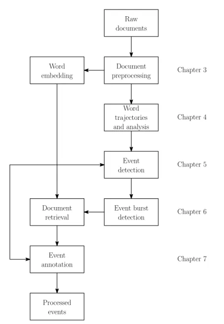
The rest of the thesis is organized as follows. First, in Chapter 2, we discuss related work. Then, in Chapter 3, we describe the document collection used for evaluation and the preprocessing steps taken.

In Chapter 4, we describe the original paper’s procedure used to extract temporal characteristics of the individual words. These characteristics are then examined to reveal a subset of words which may be related to certain events, as opposed to generally appearing noisy words, so called stopwords.

Then, in Chapter 5, we proceed to the event detection itself. Here, we describe the original method, its modification relying on word embedding and also propose

an alternative algorithm for event detection.

Although a set of related keywords provides a concise event representation, it is not particularly readable to the user. In Chapter 6, we follow by interpreting each keyword set as a query to the document collection. This allows us to employ Information Retrieval techniques to obtain documents relevant to each event.

Since the number of documents may be still too high, we also generate a short annotation for each event. The user can quickly skim through these annotations to get an idea what the events are about, and decide which of them are worth a closer examination. This will be addressed in Chapter 7.

Finally, we evaluate our method and compare it to the original paper in Chap-ter 8. We then conclude the thesis in ChapChap-ter 9.

Event annotation Word embedding Document preprocessing Event detection Event burst detection Document retrieval Chapter 3 Chapter 4 Chapter 5 Chapter 6 Chapter 7 Raw documents Word trajectories and analysis Processed events

Chapter 2

Related work

A system encompassing event detection, subsequent document retrieval and auto-matic event annotation needs to tackle several issues. In particular, we need to select a suitable word embedding model to be used during the detection. Furthermore, we must decide on the detection method itself and also specify the process of relevant documents retrieval. Finally, we need to find a suitable method of annotating the detected events in a human-readable fashion.

All of these concerns have been addressed in literature. Below, we provide a basic overview of the related work which was helpful for our approach.

2.1

Word embedding

Recently, a number of neural network models for vector space word embedding have been proposed. Perhaps the best known model is Word2Vec (Mikolov et al., 2013a) by Tom´aˇs Mikolov. Additional methods include Stanford GloVe (Pennington et al., 2014), WordRank (Ji et al., 2015) and FastText (Bojanowski et al., 2016).

In this thesis, we use the Word2Vec model. The learned word vectors have useful semantical properties (Mikolov et al., 2013b,c), an efficient implementation exists ( ˇReh˚uˇrek and Sojka, 2010), and it is a well documented and accepted method.

The Word2Vec model has additionally been modified to support embedding whole documents (Le and Mikolov, 2014).

2.2

Event detection

Although our method is evaluated on a news collection, the documents do not nec-essarily have to come from a formal news source. A lot of work has also been published in event detection by analyzing tweets, an overview can be found in Ate-feh and Khreich (2015), other examples being Ifrim et al. (2014) and Brigadir et al. (2014). Atefeh and Khreich (2015) also distinguish betweenretrospective and online

event detection. The former analyzes a given collection of documents to discover past events, the latter (also known as First Story Detection) tries to classify contin-uously incoming texts into “old” documents concerning events already known, and “new” documents concerning events not yet seen.

Further distinction can be made based on event representation. Some methods directly compare documents by their content and temporal similarity (He et al.,

2007b), outputting an event as a set of documents. Others, such as Fung et al. (2005); He et al. (2007a); Fisichella et al. (2011) and our method included, represent the events by clusters of semantically and temporarily related keywords.

Additional work has also been done in event detection through topic modeling (Chaney et al.; Keane et al., 2015). Topic modeling will be briefly addressed in the next section.

2.3

Document retrieval

Retrieving relevant documents from a large corpus based on a user-given query is the main concern of Information Retrieval (Rijsbergen, 1979; Manning et al., 2008). A number of methods comparing similarity of document representation through vectors has been created. These methods range from a simple, yet precise binary weighting (Luhn, 1957; Salton and Buckley, 1988; Manning et al., 2008), to those utilizing term weighting to diminish common words (Sparck Jones, 1972) and approaches that attempt to discover a latent structure behind the documents, such as Latent Semantic Indexing (Deerwester et al., 1990).

Further work has been done in topic modeling, where the focus is to discover abstract topics behind the documents. Latent Semantic Indexing belongs to topic modeling as well. More complex methods, such as Latent Dirichlet Allocation (Blei et al., 2003) employ a generative probabilistic model to discover the topical structure. Document can then be compared in terms of their topical similarity.

Recently, a new similarity measure utilizing the Word2Vec model, an extension of Rubner et al. (2000), called Word Mover’s Distance (Kusner et al., 2015) was introduced. This is a measure we are going to use and discuss in Chapter 6 in more detail.

2.4

Event annotation

For annotating the detected events, we consulted Gupta and Lehal (2010) and Nenkova and McKeown (2012). We aim to obtain a short summary for each event using the documents retrieved as relevant. The task of document summarization can be divided into abstractive, where the task is to generate new sentences or words not seen in the documents, and extractive, where the task is to extract parts of the document into a summary.

An example of the abstractive approach applied on news events is Alfonseca et al. (2013), extractive approach is addressed by e.g. Ferreira et al. (2014); Lin and Bilmes (2010, 2011). The abstractive methods are much more complex and still an active area of research, as it is necessary to generate sentences with a logical structure. We decided to employ the extractive approach, as the methods are generally better documented, simpler and more mature.

The method introduced by Lin and Bilmes (2010, 2011) supports multi-document summarization, which is suitable for our task, as we have multiple documents rele-vant to each event. Additionally, K˚ageb¨ack et al. (2014) examined various ways of how this approach could be improved by word embeddings. Their work led to a sys-tem presented in Mogren et al. (2015) which aggregates multiple similarity measures to perform summarization. We decided to adapt this system for our task.

Chapter 3

Document stream and

preprocessing

The document collection we work with comes directly from webscraping various Czech news servers, and does not have any special structure. The documents consist only of headlines, bodies and publication days. Furthermore, there are some noisy words such as residual HTML entities, typos, words cut in the middle, etc. To make the most of the collection, we preprocess the documents to remove as many of these errors as possible, and also to gain some additional information about the text.

We first employ some NLP (Natural Language Processing) methods to gain in-sight into the data. Then, we train a model to obtain word embeddings, which we discuss next.

Our event detection method is keyword-based — the events will be represented by groups of keywords related in the temporal as well as semantic domain. To be able to measure the semantic similarity, we need to obtain a representation of the individual words that retains as much semantic information as possible while sup-porting similarity queries. There is a number of ways to do so — a simple TFIDF (Term Frequency-Inverse Document Frequency) representation (Sparck Jones, 1972; Manning et al., 2008) which represents the words by weighted counts of their ap-pearance in the document collection. More complicated methods, such as Latent Semantic Indexing (Deerwester et al., 1990) attempt to discover latent structure within words to also reveal topical relations between them. This idea is further pursued by probabilistic topical models, such as Latent Dirichlet Allocation (Blei et al., 2003).

In this thesis, we use the Word2Vec model introduced by Mikolov et al. (2013a,b,c), which uses a shallow neural network to project the words from a predetermined vocabulary into a vector space. Vectors in this space have interesting semantical properties, such as vector arithmetics preserving semantic relations, or semantically related words forming clusters. A useful property of the Word2Vec model is that it supports online learning, meaning that the training can be stopped and resumed as needed. We can then train the model on one document collection, and only perform small updates when we receive new documents with different vocabulary.

Later on, we will need some sort of word similarity measure. This will come up several times in the course of the thesis — in the event detection itself, later when querying the document collection to obtain document representation of the events detected, and finally when generating human-readable summaries. The Word2Vec

model is fit for all of these uses, as opposed to the other approaches mentioned above, some of which are designed only to measure document similarity, or, on the other hand, do not support document similarity queries very well.

3.1

Preprocessing

Some of the documents contain residual HTML entities from errors during web scraping, which we filter out using a manually constructed stopwords list.

We used the MorphoDiTa tagger (Strakov´a et al., 2014) to perform tokenization, lemmatization and parts of speech tagging. Our whole analysis is applied to these lemmatized texts; we revert to the full forms only at the end when annotating the events in a human-readable way.

3.2

Word embeddings

Next, we train the previously mentioned Word2Vec model. Although the training is time-consuming 1, the word vectors can be pre-trained on a large document col-lection and then reused in following runs. In case the vocabulary used in these new documents differs, the model can be simply updated with the new words.

For the training, we only discard punctuation marks and words denoted as un-known parts of speech by the tagger. Such words are mostly typos not important for our analysis. We also discard words appearing in less than 10 documents.

The thesis was implemented using the Gensim ( ˇReh˚uˇrek and Sojka, 2010) library. The project contains memory efficient, easy to use Python implementations of vari-ous topic modeling algorithms, Word2Vec included. In addition, we used the SciPy toolkit (Jones et al., 2001–) and Scikit-Learn (Pedregosa et al., 2011) for various machine learning-related computations.

We use the skip-gram model defined in Mikolov et al. (2013a), which was shown in Mikolov et al. (2013b) to learn high quality word embeddings well capturing semantic properties. After experimenting with different settings on a smaller subset of the documents, we decided to embed the words in a 100-dimensional vector space and to allow 5 passes over the document collection. Allowing more passes slows down the training, while not improving the quality very much. Setting higher dimensionality also does not lead to significant quality improvement, and slows down the training as well as requires more memory.

In the thesis, we refer to the vector embedding of a word w asvw ∈R100.

3.3

Document collection

The dataset used is a collection of Czech news documents from various sources accumulated over a period from January 1, 2014 to January 31, 2015. The collection contains 2,078,774 documents averaging at 260 words each, with 2,058,316 unique word tokens in total. However, majority of the words are rare words or typos of no importance, so the number of unique real words is much lower. This is confirmed

after discarding the words appearing in less than 10 documents, with only 351,136 unique words remaining.

These words are further processed in the following chapter, where we uncover a small subset of words possibly representative of an event, and discard the rest.

3.4

Document stream formally

Formally, the input to the algorithm is a collection ofN news documents containing full text articles along with their publication days and headlines.

If we denote ti as the publication day of a document di, the collection can be

understood as a stream {(d1, t1),(d2, t2), . . . ,(dN, tN)} with ti ≤ tj for i < j.

Fur-thermore, we define T to be the length of the stream (in days), and we normalize the document publication days to be relative to the document stream start; that is

Chapter 4

Word-level analysis

Word-level analysis is the first phase of the event detection algorithm, focused on ob-taining temporal characteristics of the individual words as well as a set of candidate words for event representation. We do not yet perform the actual event detection, which is addressed in the next chapter, but merely extract a subset of words carrying enough information to be considered representative.

Here we work with the assumption that an event can be detected by observing the frequencies of individual words over time and grouping together those words which appear in similar documents during similar time periods (He et al., 2007a; Fung et al., 2005). This corresponds to an event being often mentioned in the text stream around the period when it actually occurred. Of course, not all words are representative of an event, so we will have to impose a criterion of a “word eventness”.

He et al. (2007a) also distinguished between periodic and aperiodic words, where periodic words are mentioned with a certain period (these words are related for example to sport matches played every weekend, weather forecasts reported every day, etc.) Consequently, the authors divided the words into two groups by their periodicity, and detected events from each group separately. However, during our evaluation, some word periodicities were misclassified. This would cause an event represented by those words to be split into a “periodic part” and an “aperiodic part”. Therefore, we detect events from all “eventful” words at once, and examine the periodicities of the events later on in Chapter 6.

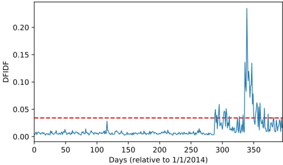
We show an example of such periodicity misclassification in Figure 4.1. There are two words representing the same real world event, the first of which in Figure 4.1a being correctly classified as aperiodic. The word in Figure 4.1b also has a distinct burst of activity typical for aperiodic words, though it is labeled periodic due to the noise present in its time trajectory. If we detected the events separately from the aperiodic and periodic categories, these two words could not be assigned together, even though they concern the same event.

At first, we construct a time trajectory of each word — a measure of word frequency over time. Then, we apply signal processing techniques to determine the eventness of each word. The same techniques will be later used to determine the event periodicities in Chapter 6. Once we have a notion of word eventness, we extract a small subset of words to be considered for further analysis, and discard the rest.

0 50 100 150 200 250 300 350 Days (relative to 1/1/2014) 0.0 0.1 0.2 0.3 0.4 0.5 DF IDF Hebdo

(a) Aperiodic word

0 50 100 150 200 250 300 350 Days (relative to 1/1/2014) 0.00 0.05 0.10 0.15 0.20 0.25 DF IDF islám

(b) Aperiodic word misclassified as periodic

Figure 4.1: Trajectories of the words Hebdo and Islam, respectively. Both of these words are related to the shooting in Charlie Hebdo offices in Paris on January 7, 2015. However, the original method classifies the wordIslamas periodic with period of 198 days. If we detected events separately from periodic and aperiodic words, the event “Charlie Hebdo attack” would be split into at least two, causing redundancy.

where a word would suddenly start appearing in a large number of documents dur-ing a short time period. Should a number of words appear in similar documents with overlapping bursts, it may be an indicator that an event worthy of attention occurred.

One thing to note is that the frequency of a word is, by itself, not a good indicator of a word importance. Stopwords appearing in most documents, such as conjunctions, prepositions, etc. do not carry any information and should be ignored. Therefore, we utilize the parts of speech tagging performed earlier and limit our analysis to Nouns, Verbs, Adjectives and Adverbs only. This limits the number of stopwords appearing in the stream, though some remain. These will need to be filtered by other means, as we will see later in this chapter.

We compare the trajectories of a typical eventful word and a stopword in Fig-ure 4.2. The trajectory of the eventful word contains a distinct burst of activity, indicating a possible event happening. The stopword, on the other hand, does not contain such bursts, its trajectory oscillating as the word is mentioned in many doc-uments over time. Although there are eventful periodic words with multiple bursts as well, as in Figure 4.3a, their trajectories generally reach higher values than those of stopwords. This difference in values will be used to distinguish stopwords from eventful words in Section 4.3.

We ignore the documents and focus entirely on word analysis up until Chapter 6. There, we use the words assembled into events to query the document collection, obtaining the event-related documents. The core of the word analysis algorithm is taken from He et al. (2007a).

4.1

Binary bag of words model

To construct the word trajectories, we first need to know which words appear in which documents, as we are interested in the document frequency of each word. We create a binary bag of words model, which is represented by a binary matrix denoting the incidence of documents and words. This model completely ignores

0 50 100 150 200 250 300 350 Days (relative to 1/1/2014) 0.00 0.25 0.50 0.75 1.00 1.25 DF IDF Vánoce (Christmas)

(a) Eventful word

0 50 100 150 200 250 300 350 Days (relative to 1/1/2014) 0.05 0.10 0.15 0.20 0.25 DF IDF pátek (Friday) (b) Stopword

Figure 4.2: (a) Trajectory of an eventful word Christmas. (b) Trajectory of a stopword Friday with a period of 7 days.

word order, which is neglected in this analysis.

It might seem that using only a simplebinary model, as opposed to one denoting, say, the frequency of words within the documents, results in a loss of information. While true, this model is not the target word representation — we only need to know the word-document incidence to construct the word trajectories, which are then the desired output.

We define a term-document matrix B ∈ {0,1}N×V, where N is the number of documents and V is the total vocabulary size. The document collection can then be interpreted as a set ofN observations, each consisting ofV binary features. The matrix B is defined as

Bij = (

1, document i contains the wordj;

0, otherwise. (4.1)

Because every document contains only a small fraction of the vocabulary, the matrix B consists mostly of zeroes. This allows us to store the matrix in a sparse format, which makes it possible to fit the matrix in memory. We use a sparse matrix instead of a more traditional inverted index (Manning et al., 2008), because this representation allows us to vectorize some further operations.

4.2

Computing word trajectories

He et al. (2007a) defined the time trajectory of a word was a vector

y_w = [yw(1), yw(2), . . . , yw(T)] with each elementyw(t) being the relative frequency

ofw at time t (1≤t ≤T, 1≤w≤V). This frequency is defined using the DFIDF (Document Frequency-Inverse Document Frequency) score:

yw(t) = DFw(t) N(t) | {z } DF ·log N DFw | {z } IDF , (4.2)

where DFw(t) is the number of documents published on daytcontaining the word w (time-local document frequency), N(t) is the number of documents published on day t, N is the total number of documents and DFw is the number of documents

The DFIDF score, defined by He et al. (2007a), is a modification of the commonly used TFIDF (Term Frequency-Inverse Document Frequency) score (Sparck Jones, 1972; Manning et al., 2008), which measures the importance of a word within a docu-ment collection. The purpose of this modification is to include temporal information and measure the word importance over time.

To be able to compute these word trajectories efficiently using the matrixB, we define a utility matrix D ∈ {0,1}N×T mapping the documents to their publication days:

Dij = (

1, document i was published on dayj;

0, otherwise. (4.3)

Next, we sum the rows ofBtogether to obtaindf = [DF1,DF2, . . . ,DFV]; DFj = PN

i=1Bij. Similarly, we sum the rows of D to obtain nt = [N(1),N(2), . . . ,N(T)];

N(j) =PN i=1Dij.

Finally, we compute the word trajectory matrixY ∈_RV×T_{, with trajectory of a}

word w, y_w ∈_RT_{, being the w-th row of Y.}

The matrix Y is computed as follows:

Y = diag log N df | {z } IDF ·BT·D·diag 1 nt | {z } DF (4.4)

Now, having trained the Word2Vec model in Chapter 3 and constructed the word trajectories, we obtained temporal and semantic representation of the words. Every word w is represented by two vectors: vw ∈ R100 being its Word2Vec embedding,

and y_w ∈ _RT _{its time trajectory. The trajectories will be further analyzed in this}

chapter, while both trajectories and Word2Vec embeddings will be used in Chapter 5 to group words into events.

4.3

Spectral analysis

Having constructed the word trajectories, we still need to decide which words are eventful enough. He et al. (2007a) interpreted the word trajectories as time signals, which allowed them to analyze the trajectories using signal processing techniques. They performed the analysis both to decide word eventness and to discover the word periodicity.

Unlike the original paper, we only analyze the signal power to decide which words are eventful enough. We will detect events from both periodic and aperiodic words at once, and decide the periodicity of the whole events in Chapter 6.

We apply the discrete Fourier transform to the trajectories to represent each time series as a linear combination of T complex sinusoids. We obtain Fy_w = [X1, X2, . . . , XT] such that Xk= T X t=1 yw(t) exp − 2πi T (k−1)t , k= 1,2, . . . , T. (4.5)

The measure of “eventness” of a word is simply its signal power. That can be determined from the power spectrum of each signal, estimated using the periodogram

p=kX1k2,kX2k2, . . . ,kXdT /2ek2

.

To measure the overall signal power, we define the dominant power spectrum of the wordw as the value of the highest peak in the periodogram, that is

DPSw = max

k≤dT /2ekXkk

2_{. (4.6)}

In Figure 4.3, we show the trajectory and periodogram of a periodic word air-plane. In the periodogram plot, the DPS value of approximately 0.1192 is high-lighted. This value is attained at frequency of about 0.0076, making the dominant period of the word 1/0.0076 ≈ 132. Although He et al. (2007a) further utilized these dominant periods to categorize the words by their periodicities, we postpone the periodicity analysis to event trajectories assembled in Chapter 6.

0 50 100 150 200 250 300 350 Days (relative to 1/1/2014) 0.0 0.1 0.2 0.3 0.4 0.5 DF IDF letadlo (airplane) (a) Trajectory 0.0 0.1 0.2 0.3 0.4 0.5 Frequency 0.00 0.02 0.04 0.06 0.08 0.10 0.12 Pe rio do gra m letadlo (airplane)

(b) Periodogram with indicated DPS

Figure 4.3: Trajectory and periodogram of the word airplane with a period of 132 days.

Finally, He et al. (2007a) define the set of all eventful words (EW) as those words whose trajectory signal is powerful enough. This corresponds to their occurrence in a large number of documents in a noiseless pattern:

EW ={w|DPSw >DPS-bound}. (4.7)

whereDPS-bound can be estimated using theHeuristic stopword detection algo-rithm described in He et al. (2007a). The algoalgo-rithm computes the average trajectory value and DPS values from a given seed stopwords set. The DPS boundary is then defined as the maximum DPS value of the stopwords set.

Chapter 5

Event detection algorithms

In this chapter, we define the actual event detection algorithm. First, we describe the original method used by He et al. (2007a). Then, we make a change to incorporate semantic similarity through the word embeddings obtained in Chapter 3. Finally, we introduce an alternative algorithm that utilizes word clustering using a custom distance function.

The original algorithm creates events as sets of related keywords by greedily minimizing a cost function combining temporal and semantical distance between words. However, the paper used only a simple notion of semantical distance, namely the document overlap between words. This demands that there exists at least one document containing all the words used to represent an event. This is a strong requirement, since the documents may use different vocabularies while conveying similar information. As a result, the events are split into multiple keyword sets, leading to redundancy.

In an attempt to solve this problem, we modify the cost function, replacing the document overlap by a Word2Vec-based similarity. This does not require the words to appear in exactly the same documents, only that they have similar semantics. We refer to this method asembedded greedy approach, as it is a modification to make the original greedy algorithm utilize word embeddings.

Realizing that the task of constructing keyword sets resembles the task of word clustering, we propose an alternative algorithm. Here, we apply a clustering algo-rithm to the words, using a modification of the cost function as a distance measure. This is a method referred to as cluster-based approach.

First, we briefly describe the original method for reference. This will make it clear which parts of the function we modify. It will also allow us to make reference to the original method in Chapter 8, where we compare all three algorithms.

5.1

Original method

As stated in the introduction, the original method performs greedy minimization of a cost function defined over sets of words. The cost function consists of tra-jectory distance measuring the word distance in temporal domain, and document overlap, standing for distance in the semantic domain. We first describe these two components and then combine them into the cost function.

5.1.1

Trajectory distance

Before measuring the trajectory distance, the trajectories are smoothened by fitting a probability density function to them. We adapt a similar technique in Chapter 6 where it is described in more detail. Our event detection modifications do not use the original smoothing though, and we refer the reader to the original paper for more details.

After normalization to unit sum, the (smoothened) trajectory y0_w of a word w

can be interpreted as a probability distribution over the stream days. The element

y_w0 (i) then denotes the probability that wappears in a random document published on day i. This interpretation allows to compare the trajectories using information-theoretic techniques, notably the information divergence (Cover and Thomas, 2012). In the original paper, the authors first defined the distance between trajecto-ries of two words v and w as Dist(y0_v,y0_w) = max{KL(y0_vky0_w),KL(y0_wky0_v)}, symmetrizing the Kullback-Leibler divergence KL (Kullback and Leibler, 1951).

Then, the distance is generalized to a whole set of words M as

Dist(M) = max v,w∈MDist(y 0 v,y 0 w). (5.1)

5.1.2

Document overlap

The document overlap is again first defined for a pair of wordsvandwas DO (v, w) =

|Mv∩Mw|

min{|Mv|,|Mw|}, where Mj = {i | Bij = 1} is the set of all documents containing the

word j. The higher the document overlap, the more documents do the two words have in common, which makes them more likely to be correlated.

The overlap is again generalized to a set of words M as

DO(M) = min

v,w∈MDO(v, w). (5.2)

5.1.3

Cost function

The cost function is a combination of the trajectory distance and document overlap of a set of words M. It is defined as

C(M) = Dist(M) DO(M)·P

w∈MDPSw

. (5.3)

Since the algorithm attempts to minimize it, the intuitive result is a set of words with low trajectory distance and high document overlap. The algorithm will also prefer words of higher importance due to the last term of the denominator, counting in the power spectra.

5.1.4

Event detection algorithm

The algorithm, called unsupervised greedy event detection algorithm in the original paper, produces events as structured objects e consisting of:

• e.KW: The event keyword set.

• e.Bursts: Bursty periods of the event. • e.DP: Dominant period of the event.

• e.Annotation: Human-readable annotation of the event.

Only the event keyword set e.KW is initialized in this section. The other fields will be properly defined and filled in the rest of the thesis.

The algorithm itself is defined as follows:

Algorithm 1 Unsupervised greedy event detection

Input: Word set EW obtained in Chapter 4, matrices B and Y, word DPS

1: Sort the words in descending DPS order: DPSw1 ≥ · · · ≥DPSw|EW|

2: k = 0 3: for each w∈EW do 4: k=k+ 1 5: ek.KW ={w} 6: costek = 1 DP Sw 7: EW = EW\w 8: while EW6=∅ do 9: m= argmin m C(ek.KW∪wm) 10: if C(ek.KW∪wm)< costek then 11: costek = C(ek.KW∪wm) 12: ek.KW=ek.KW∪wm 13: EW = EW\wm 14: else 15: break 16: end if 17: end while 18: end for Output: Events {e1, . . . , ek}

The algorithm works by greedily minimizing the cost function (5.3). Once it is minimized, an event is produced, consisting of all the words found since last event. The words are sorted in descending DPS order before entering the minimization loop, so that the most important words are processed first. This assures that the most eventful words are assigned together, without wasting them to appear with low quality words.

He et al. (2007a) did not provide the time complexity of the algorithm, which we attempt to estimate now. The execution time is dominated by the main loop on lines 3 through 18. The outer loop must execute O(|EW|) times. In each of the iterations, the inner loop is executed at most |EW| times, making it O(|EW|) as well. The argmin statement on line 9 must search through the whole remaining |EW| words, also making it run O(|EW|) times.

If the number of eventful words is low enough, the pairwise trajectory distance and document overlap can be precomputed. This makes the cost function take O(|M|2_{) time when applied to a set M. If the distances are not precomputed, the}

0 50 100 150 200 250 300 350 Days (relative to 1/1/2014) 0.00 0.05 0.10 0.15 0.20 0.25 0.30 DF IDF palestinský izraelský Palestinec Izrael

Figure 5.1: Example of an event detected using the original method. The event consists of the words palestinian, israeli,Palestinian and Israel, respectively.

We were unable to precisely determine the cost function’s complexity with re-spect to the set EW, as it is always applied on the currently composed event. However, during our experiments, the number of words comprising an event never exceeded 10 in the original method. This makes the cost function’s asymptotic complexity negligible compared to the main loop.

The resulting complexity of the algorithm is therefore O(|EW|3 _{·c), where c is}

the complexity of the cost function.

In Figure 5.1, we show an example of an event detected by the original method. We can see that it consists of four keywords with overlapping trajectories, sharing a common burst of activity around day 210. The event is likely related to the tension in the Middle East, though the keywords by themselves do not allow any closer interpretation. For this reason, we provide longer annotations in Chapter 7, so that we can examine the event more closely.

5.2

Embedded greedy approach

In this section, we modify the original method to use the Word2Vec model to measure semantic similarity between words. Unlike the document overlap (5.2), this new similarity measure is able to distinguish semantically similar words even when they do not appear in the same documents. This may happen, for instance, when different authors each use distinct vocabulary when referring to the same event.

5.2.1

Semantic similarity

Some of the astounding results of the Word2Vec model arise from semantically similar words forming clusters (Mikolov et al., 2013c) in terms of cosine similarity, which is a standard measure used in information retrieval (Manning et al., 2008;

Huang, 2008).

We replace the document overlap in the cost function (5.3) by cosine similar-ity between Word2Vec embeddings, though with a small modification. The cosine similarity is bounded in [−1,1] with -1 denoting the least degree of similarity. This means that the cost function would reach negative values for highly dissimilar words. This would mean a problem, as Algorithm 1 attempts to minimize it. Consequently, we will transform the cosine similarity into [0,1], just like the document overlap (5.2).

The similarity between a set of words M and a wordw /∈M is defined as

Sim(M, w) = ¯ vM,vw k¯vMk · kvwk + 1 ! / 2, (5.4)

where ¯vM is the mean of all vector embeddings of M and vw is the vector

em-bedding of w. Here, the mean vector virtually represents the central topic of words in M.

5.2.2

Cost function

We redefine the cost function (5.3) as

C(M, w) = Dist(M∪w) Sim(M, w)·P

u∈M∪wDPSu

, (5.5)

where Dist(·) is the original trajectory distance function (5.1).

In the original method, He et al. (2007a) defined the cost function (5.3) for a set of words. However, in Algorithm 1, it is always applied on the union of the keywords of an event constructed so far, and a newly added word. The new cost function must now be applied on such keyword set and word separately due to the nature of Word2Vec similarity definition.

Having constructed the cost function, we use Algorithm 1 to detect events once again.

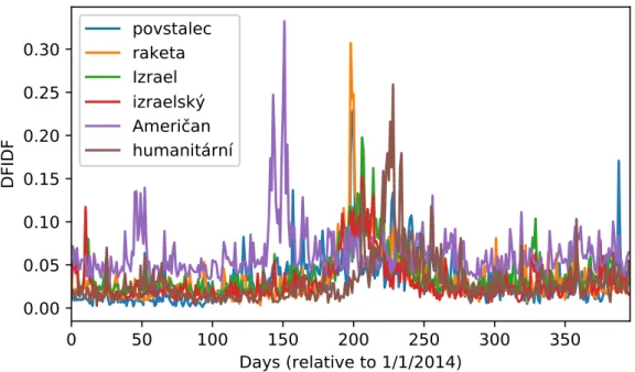
In Figure 5.2, we show an event detected using the embedded greedy method. It is related to the same real-world event as the event in Figure 5.1, though it consists of more keywords. Generally, events detected by the embedded greedy method contain more keywords, as we will see in Table 8.1. The trajectory overlap is not perfect, the burst of the word American being off compared to the rest of the words. It is possible that the semantic similarity of the word was so high that the word was deemed relevant nonetheless.

5.3

Cluster-based approach

Realizing that the keyword-based event detection resembles word clustering and could be solved by an application of a clustering algorithm, we decided to investigate this idea. In the final method, we apply a clustering algorithm equipped with a custom distance function to the set of eventful words. The distance function is actually a modification of the cost function yet again, though some means have to be taken to make it usable in this context. First though, we need to consider a proper clustering algorithm.

0

50

100

150

200

250

300

350

Days (relative to 1/1/2014)

0.00

0.05

0.10

0.15

0.20

0.25

0.30

DF

IDF

povstalec

raketa

Izrael

izraelský

Američan

humanitární

Figure 5.2: Example of an event detected using the embedded greedy method. The event consists of the wordsrebel, missile, Israel, israeli, American andhumanitarian, and is related to the same real event as Figure 5.1.

The obvious requirement for the clustering algorithm is that it must require no prior knowledge of the desired number of clusters. Another requirement is that the algorithm must accept a custom distance measure.

We considered three candidate algorithms, all satisfying these requirements: Affinity propagation (Frey and Dueck, 2007), DBSCAN (Ester et al., 1996) and its modification, HDBSCAN (Campello et al., 2013).

During our experimentation, Affinity propagation performed poorly, its clusters being often seemingly random and of low quality. The quality of HDBSCAN clus-ters was considerably better, though the algorithm took longer to converge as the number of eventful words grew. It also required to tune multiple parameters, which was difficult to do without any annotated data. We decided to use the DBSCAN algorithm, which outperformed Affinity propagation as well, and does not require to tune as many parameters as HDBSCAN.

In addition to the previously stated requirements, DBSCAN is also capable of filtering out noisy samples (in our case words), not fit for any of the clusters. This property will prove advantageous for our task, as will become clear during the eval-uation in Section 8.3.

5.3.1

Noise filtering

Before we apply clustering, we filter out the noisy parts from the word trajectories. Most words are on some level reported all the time, though only a fraction of these reportings corresponds to notable events. Unlike the greedy optimization described previously, clustering is prone to such noise, and would yield clusters of poor quality, often with trajectories being put together only due to their noisy parts being similar. Additionaly, with DBSCAN capable of filtering out noisy samples, some high quality words could be discarded precisely due to this noise in their (otherwise eventful)

trajectories.

We want to keep only those trajectory parts exceeding a certain frequency level, distinguishing notable bursts from the general noise. We do this by computing a cutoff value for each event trajectory and discarding the sectors falling under this cutoff. This procedure is adopted from Vlachos et al. (2004). The algorithm is based on computing a moving average along the trajectory, and works as follows:

Algorithm 2 Burst filtering

Input: Window-length l, word trajectory yw

1: mal = Moving Average of length l for yw = [yw(1), yw(2), . . . , yw(T)]

2: cutoff = mean (mal) + std (mal)

3: burstsw = [yw(t)|yw(t)>cutoff]

Output: burstsw

We use the window lengthl = 7, looking 1 week back in the trajectory.

5.3.2

Distance function

We now define the distance function used by DBSCAN. It conveys similar informa-tion as the cost funcinforma-tion in the previous two algorithms. We still need to measure the trajectory distance as well as semantic similarity between words, though the distance will now be defined strictly pairwise.

For a measure of trajectory distance, we replace the Kullback-Leibler divergence by the Jensen-Shannon divergence JSD (Lin, 1991), which is symmetric in its argu-ments. This is a necessary property of the distance function.

Although He et al. (2007a) did symmetrize the Kullback-Leibler divergence, they did not provide any source for their symmetrization form. We were unable to find a case where that particular form was used, though we discovered the Jensen-Shannon divergence, which comes from stronger mathematical background (Lin, 1991; Fu-glede and Topsoe, 2004). It also tended to improve the clustering quality during our experimentation, as opposed to the original symmetrization. We then decided to replace the original paper’s KL-divergence symmetrization by the JS-divergence. Instead of semantic similarity, we measure semantic distance as the Euclidean distance between two word vector embeddings. The reason is that Euclidean dis-tance is unbounded, which makes it possible for the samples to be spread farther apart. Since DBSCAN is a density-based clustering algorithm, having high density areas consisting of words with low trajectory distance and similar cosine similarities would cause them to appear in the same cluster. This would cluster the words only in terms of their trajectories, not semantics.

The distance between two words v and w with (normalized and filtered using Algorithm 2) trajectories y0_v, y0_w and Word2Vec embeddingsvv, vw is now defined

as

d(v, w) = JSD(y0_vky0_w)· kvv−vwk2, (5.6)

0

50

100

150

200

250

300

350

Days (relative to 1/1/2014)

0.00

0.05

0.10

0.15

0.20

0.25

0.30

DF

IDF

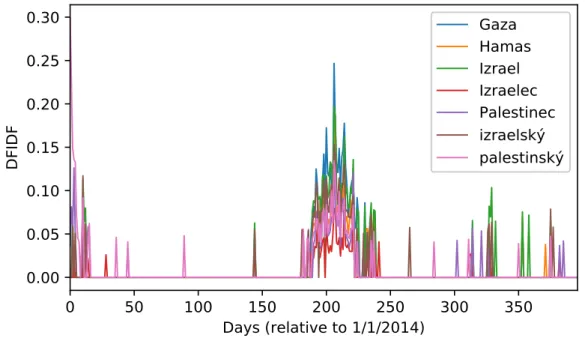
Gaza

Hamas

Izrael

Izraelec

Palestinec

izraelský

palestinský

Figure 5.3: Example of an event detected using the cluster-based method. The event is related to the same real event as Figure 5.1 and Figure 5.2.

5.3.3

Event detection

Now, we describe the cluster-based event detection algorithm, which is a direct application of the DBSCAN algorithm and consequent noise filtering.

Algorithm 3 Cluster-based event detection

Input: Word set EW obtained in Chapter 4, matrix Y, word embeddings for EW

1: Precompute a distance matrixDist∈_R|EW|×|EW| _{with Dist}

ij = d(wi, wj)

2: Apply DBSCAN toDist, obtaining k clusters and the noisy cluster

3: for each(w, cluster)∈DBSCAN.clusters do

4: if cluster 6=noise then

5: ecluster.KW =ecluster.KW∪w

6: end if

7: end for

Output: Events{e1, e2, . . . , ek}

In Figure 5.3, we show an event detected using the cluster-based method. It is again related to the same real event as those in Figure 5.1 and Figure 5.2. The main thing to note is that the word trajectories are clear of noise due to application of Algorithm 2. This made it possible to match words only based on their bursts, not any underlying noise. Compared to the event depicted in Figure 5.2, the cleaned trajectories overlap almost perfectly.

Chapter 6

Document retrieval

Having detected the events, we still have to present them to the user in a readable format. A set of keywords may be a concise representation for the computer, but it does not offer much insight into the event itself. We aim to generate short anno-tations for the events, based on which the user can decide to actually inspect the event more thoroughly and read some of the documents. Consequently, we need to retrieve a number of documents relevant to each event. These documents will then be used in Chapter 7 to generate summaries.

We can use each event’s temporal and semantic information to query the doc-ument collection. The former is trivial – simply select the docdoc-uments published within an event’s bursty period. From these document, we can then select those document which relate to the event semantically. This will prove more complicated, and we will need to employ some more information retrieval techniques to obtain the documents.

As of now, an eventeis described by a set of its keywords,e.KW. The goal is to convert this keyword representation to a document representation,e.Docsconsisting of documents related to e.

6.1

Event burst detection

First, we need to detect the period when the particular event happened, so that we can retrieve the documents published around that time. This part of the algorithm again follows from He et al. (2007a). In this paper, the period around an event’s occurrence was called bursty period. The burst detection is done in five steps.

1. Construct the event trajectory from the trajectories of its keywords.

2. Clean the event trajectory.

3. Determine the event’s periodicity.

4. Fit a probability density function to the event trajectory.

0 50 100 150 200 250 300 350 Days (relative to 1/1/2014) 0.0 0.1 0.2 0.3 0.4 0.5 DF IDF

(a) Event keywords

0 50 100 150 200 250 300 350 Days (relative to 1/1/2014) 0.00 0.05 0.10 0.15 0.20 0.25 0.30 DF IDF (b) Event trajectory

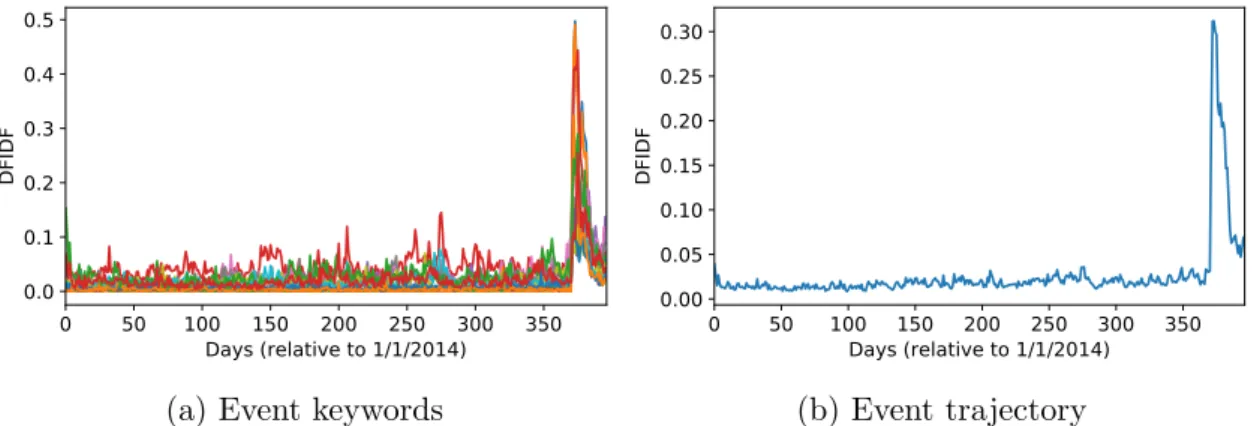
Figure 6.1: Keywords and trajectory of the event related to Charlie Hebdo attack. The keywords are Charlie, Hebdo, Mohamed (Muhammad), Paˇr´ıˇz (Paris), Islam, karikatura (caricature), Muslim, n´aboˇzenstv´ı (religion), paˇr´ıˇzsk´y (Parisian), prorok (prophet), satirick´y (satirical), teroristick´y (terroristic), terorizmus (terrorism).

6.1.1

Event trajectory construction

We first need to construct an event trajectory out of its keyword trajectories. We do this by computing a weighted average of the event’s keyword trajectories, with weights being the keyword DPS. This ensures that less important words with slightly different time characteristic will not shift the trajectory away from the actual burst.

ye= 1 P k∈e.KWDPSk X k∈e.KW DPSk·yk (6.1)

An example of such event trajectory can be found in Figure 6.1.

6.1.2

Trajectory filtering

Now, a typical event (shown in Figure 6.2) usually has a number of dominant bursts corresponding to the period(s) when the event actually occurred. Additionally, there are some milder, noisy bursts due to the keywords appearing elsewhere, indepen-dently of that particular event.

We aim to fit a probability density function to the event trajectory, as in He et al. (2007a). The noisy bursts would behave as outliers, shifting the fitted function away from the main event bursts. Once again, we apply the Burst filtering algorithm from Subsection 5.3.1 to filter out noise, this time from the event trajectories. The cutoff value computed by the Burst filtering algorithm is shown in Figure 6.2 as well.

6.1.3

Event periodicity

We apply the signal processing techniques described in Chapter 4 once more, this time to determine the dominant period e.DP of each event e. After computing the periodogram, the dominant period is defined as the inverse of the frequency corresponding to the highest peak in the event trajectory:

e.DP= T

argmax

k≤dT /2e

kXkk2

0 50 100 150 200 250 300 350 Days (relative to 1/1/2014) 0.00 0.05 0.10 0.15 0.20 DF IDF

Figure 6.2: An event with a noisy trajectory and keywords Vrbˇetice, muniˇcn´ı (am-munition), sklad (storage) related to the explosions of the ammunition storage in Vrbˇetice on October 16 and December 3, 2014 (events 38 and 47 in Appendix A. The dashed red line is the cutoff value computed using window length 7. The parts of the trajectory under the cutoff will be discarded.

as the Fourier coefficient Xk denotes the amplitude at frequency _Tk. We then

consider an event e to beaperiodic if it happened only once in the stream, that is if

e.DP>dT /2e. Similarly, the event is periodic if e.DP≤ dT /2e.

6.1.4

Density fitting

We normalize the event trajectories to have unit sums, so they can be interpreted as probability distribution over days. An elementy0_e(i) of the normalized trajectoryy0_e can be interpreted as the probability of that event occurring on day i. This allows us to fit a probability density function to them. He et al. (2007a) adapted a similar approach, though only for word rather than event trajectories.

We describe aperiodic and periodic events separately, as different probability distributions must be used in case of a single burst than in case of multiple bursts.

1. Aperiodic events

An aperiodic event trajectoryy0_eis modeled by a Gaussian distributionN(µ, σ2). We fit the Gaussian function to the trajectoryy0_eand estimate the parameters

µ and σ. He et al. (2007a) did not mention the method they used for ape-riodic trajectories. As we are fitting the density to probabilities rather than observations, Maximum Likelihood Estimate of the parameters is not appli-cable. We decided to use non-linear least squares, namely the Trust Region Reflective algorithm (Branch et al., 1999) to estimateµandσ bounded within the document stream period. An example of the Gaussian distribution fit to an event trajectory is shown in Figure 6.3.

42.7 Days (relative to 1/1/2014) 0.00 0.01 0.02 0.03 0.04 DF IDF

Figure 6.3: An aperiodic event consisting of the keywords Sochi, ZOH (Winter Olympic Games), olympijsk´y (olympic), olympi´ada (olympiad). The Gaussian func-tion modeling the trajectory and the event bursty period are shown in red.

2. Periodic events

A periodic event trajectory y0_e is modeled using a mixture of K =bT /e.DPc Cauchy distributions (as many mixture components as there are periods), as in Fisichella et al. (2011): f(x) = K X k=1 αk 1 π γk (x−µk)2+γ_k2 !

The mixing parameters αk ≥ 0, PK

k=1αk = 1, location parameters µk and

scale parameters γk are estimated using the EM algorithm.

The Cauchy distribution has a narrower peak and thicker tails than the Gaus-sian distribution, which models the periodic bursts more closely. The indi-vidual bursts of a periodic event tend to be quite short, but even between two consecutive bursts, the frequency remains at a non-negligible level, which makes the Cauchy distribution a somewhat better choice. Figure 6.4 shows an example of such fit.

6.1.5

Burst detection

Using the fitted probability density functions, we define the bursty period(s) as the regions with the highest density. The bursty period of an aperiodic event e is now defined as e.Bursts = {[µ−σ, µ+σ]}. For a periodic event, there are K = bT /e.DPc bursty periods defined as e.Bursts= {[µk−γk, µk+γk]|k = 1, . . . , K}.

The burst of an aperiodic event is highlighted in Figure 6.3, while a periodic event’s bursts are shown in Figure 6.4.

296.5 58.1 143.5 Days (relative to 1/1/2014) 0.000 0.005 0.010 0.015 0.020 0.025 DF IDF

Figure 6.4: A periodic event with keywordsvolba (election), volebn´ı (electoral), voliˇc (voter) and a period of 132 days. The event is modeled by a mixture ofb396/132c= 3 Cauchy distributions. Each of the event’s bursty periods is highlighted.

6.2

Document retrieval

We only describe the process for aperiodic events. The method is similar for periodic events, except applied on each burst individually.

We need to measure the relevance of individual documents published within an event’s bursty period to the event. The only measure of semantics for an event we have is the event’s keyword set e.KW. If we interpret e.KW as a keyword query for the document collection, we arrive at the classical task of Information Retrieval. That is, to rate the documents in a given corpus by their relevance to the query (Manning et al., 2008).

In the original method by He et al. (2007a), the task was simple due to the cost function used. The only measure of semantic similarity was the degree of document overlap between all words in e.KW. If two words had no document overlap, they would not get assigned in the same event. That way, there was always at least one document in which all of the event’s keywords appeared. It was a simple matter to compute the intersection of all documents containing either keyword within the bursty period. This is not the case in our method, and we will need to measure the document relevance in a more sophisticated way.

There are a few approaches we could take, such as project all documents and queries to a TFIDF (Term Frequency-Inverse Document Frequency) space (Man-ning et al., 2008) and sort the documents by their cosine similarity to the query. This simple approach does not go beyond a trivial keyword occurrence compari-son, though after applying some weighting scheme. We could enrich it using Latent Semantic Indexing (Deerwester et al., 1990) to also take the document topics into account. This would require us to compute yet another model to be used for this part only, which would be computationally and memory-intensive.

introduced Word Mover’s Distance (Kusner et al., 2015), which is an application of the better known measure of Earth Mover’s Distance (Rubner et al., 2000) to word embeddings.

The Word Mover’s Distance (WMD) measures the similarity of two documents as the minimum distance the word vectors of one document need to “travel” to reach the word vectors of the second document. Since more similar words are embedded close to each other (Mikolov et al., 2013c), the farther apart the words lie, the less similar they are semantically. The formal definition of the WMD is rather lengthy, so we refer the reader to the original paper (Kusner et al., 2015) for the full derivation. The WMD discards word order, which makes it suitable for our keyword queries. As the authors note, it achieves best results for short documents, in part due to the method being computationally expensive for larger pieces of text. Therefore, we apply the WMD to document headlines only.

In Information Retrieval, it is more traditional to work with document similarity rather than distance. In the Gensim framework ( ˇReh˚uˇrek and Sojka, 2010) which implements the WMD, the similarity is defined as

SimWMD(di, dj) =

1

1 + WMD(di, dj)

(6.3)

which is 1 if WMD(di, dj) = 0 and goes to 0 as WMD(di, dj)→ ∞.

We now describe the algorithm to compute the document representation of an event.

Algorithm 4 Document representation of an aperiodic event

Input: Event e, burst ∈e.Bursts, number of documentsn, document streamD

1: burst docs =∅

2: for eachdoc ∈D do

3: if doc.publication date ∈burst then

4: Compute SimWMD(e.KW,doc.headline)

5: burst docs =burst docs∪doc

6: end if

7: end for

8: Sort burst docs by the computed SimWMD in descending order

Output: first n elements of burst docs

The set of event documents e.Docs is then a union of the outputs of Algorithm 4 over all bursts in e.Bursts.

In our experiments, we chose the number of documents n as the square root of total number of documents within the particular event burst.

Chapter 7

Event annotation

The final step of our method is to annotate the detected events in a human-readable way. We aim to generate short summaries so that the user does not have to process a large quantity of text, and can just skim through a few sentences to decide whether he is interested in that particular event. If so, then he can examine the event more closely and go through the actual documents, which we have retrieved in chapter Chapter 6.

Although the keyword set discovered in Chapter 5 provides a concise representa-tion of an event, it can lead to ambiguities or simply not reveal enough informarepresenta-tion. The keywords should be considered an internal representation used in the detection process, not a feature presentable to the user.

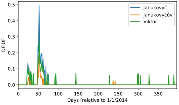
An example of such event whose background is unclear from the keyword set is shown in Figure 7.1. After manual examination, we discovered that the event concerns Viktor Yanukovych being ousted from Ukraine’s presidency, though it is unclear from the keyword set.

0 50 100 150 200 250 300 350 Days (relative to 1/1/2014 0.0 0.1 0.2 0.3 0.4 0.5 DF IDF Janukovyč Janukovyčův Viktor

Figure 7.1: An event whose meaning is not clear from the keyword set.

A simple method is to annotate an event by the headline of the most relevant document in terms of Word Mover’s Similarity. This may give insight of the general

topic of the particular event, but it is unlikely that a whole event will be well characterized by a single document. For this reason, we also investigate a more complex method.

To obtain richer annotations, we apply multi-document summarization tech-niques to generate a short summary of an event’s document set. More specifically, we attempt to extract a subset of sentences out of the event documents, which cover the general topic of the event without providing redundant information. As the documents come from different sources and describe the events from different per-spectives, the result will not generally be a continuous paragraph, but more of a set of characteristic sentences. Still, a longer piece of text will likely provide a better insight into an event than a single headline.

We examined the multi-document summarization system presented in Lin and Bilmes (2010, 2011). This system was later improved by K˚ageb¨ack et al. (2014), who evaluated the usage of different word embedding techniques for sentence similarity measures. Their work led to the system presented in Mogren et al. (2015) which aggregates several different similarity measures to obtain a better quality summary. We adapt their system and combine together several measures of sentence similarity suitable for the event detection task.

7.1

Multi-document summarization

In Lin and Bilmes (2010), the authors formulate the task of multi-document sum-marization as a constrained combinatorial optimization problem, where the goal is to retrieve a subset of sentences maximizing a monotone submodular functionF(·) measuring the summary quality.

A submodular function F(·) on a set of sentences U satisfies the property of

diminishing returns; that is, for A ⊆ B ⊆ U \ {v}, F(A∪ {v})− F(A) ≥ F(B ∪ {v})− F(B), v ∈ U. This has an intuitive interpretation for text summarization, namely that adding a sentencevto a longer summary does not improve the summary as much as adding it to a smaller one. The reason is that the information carried byv is likely already present in the longer summary.

Even though solving the task exactly is NP-hard, a greedy algorithm is guaran-teed to find a solution only a constant factor off the optimum, as discussed by the authors.

The summary quality is measured in terms of how representative it is to the whole set (coverage) and how dissimilar the sentences are to each other (diversity). The constraints limit the summary to a reasonable length by bounding the total number of words.

In Lin and Bilmes (2010), basic submodular functions to be used in multi-document summarization are described. In Lin and Bilmes (2011), these functions are further developed to better capture the semantic properties of sentences.

Mathematically, the task is formulated as

max S⊆U F(S) =L(S) +λR(S) s. t. X i∈S ci ≤ B, (7.1)

ci is the number of words in sentence i and B is the total budget, i.e. the desired

maximum summary length.

A feasible setS maximizing F(·) will provide a reasonable number of sentences well capturing the overall topic of the whole document set, no two of which being redundant. What remains is to define the coverage function L(·) and diversity func-tion R(·), whose influence can be controlled by the parameter λ≥0. Additionally, the functions must be defined in a way that the submodularity conditions from Lin and Bilmes (2010) are not violated, so that a greedy algorithm can still be used with performance guarantee.

7.2

Coverage function

In Lin and Bilmes (2011), the coverage function L(·) is defined in terms of pairwise sentence similarity Sim(·,·) as

L(S) = X i∈U minn X j∈S Sim(i, j), αX j∈U Sim(i, j) o . (7.2)

The first argument of the minimum measures the similarity between the sentence

i and the summary S, while the second argument measures the similarity between the sentence iand the rest of the sentences U. The number α∈[0,1] is a threshold coefficient controlling the influence of the overall similarity.

In Lin and Bilmes (2010), the authors further prove that if Sim(i, j)∈[0,1]∀i, j ∈

U, the whole function remains submodular.

Originally, only a simple cosine similarity between TFIDF sentence vectors (Man-ning et al., 2008) was used as Sim(·,·). K˚ageb¨ack et al. (2014) examined various methods of word embeddings to obtain a finer measure of similarity. This alone outperformed the original method. In Mogren et al. (2015), a more complex system aggregating multiple similarity measures was built, further improving the summary quality. The authors compute the sentence similarity Sim(i, j) as a product of these individual similarities, all bounded in [0,1]:

Sim(i, j) = Y

l

Ml_si,sj. (7.3)

We use this method with several different similarity measures fit for the event detection task. Next, we describe the individual sentence similarities used.

7.2.1

TFIDF similarity

The first measure used is the standard cosine similarity between TFIDF (Term Frequency-Inverse Document Frequency) vectors (Manning et al., 2008) of two sen-tences si and sj. Such method is a simple measure of document similarity often

used in information retrieval.

If we denote the frequency of the word w in sentence si as tfw,i and the inverse

document frequency of w as idfw, the similarity is written as

MTFIDF_s i,sj = P w∈si∪sjtfw,i·tfw,j ·idf 2 w q P w∈sitf 2 w,i·idf 2 w· q P w∈sjtf 2 w,j·idf 2 w . (7.4)

The term frequencies are always non-negative, and so the whole cosine similarity is in [0,1].

The major setback of TFIDF similarity is that it does not go beyond simple word overlap, though weighted to diminish stopwords and amplify important words. That means that if two sentences convey essentially the same information through different vocabulary, they will not be ranked similar due to having only a few words in common. That can be a problem in larger document collections from different sources and authors.

7.2.2

Word2Vec similarity

We attempt to solve this problem by considering the word embeddings of the indi-vidual words, as first examined by K˚ageb¨ack et al. (2014).

We represent a sentence si by summing together the vector embeddings of its

words, vi =P_w∈sivw. The similarity of two sentences is then the cosine similarity

of these vectors, transformed to [0,1]:

MW2V_s i,sj = _h vi,vji kvik · kvjk + 1 / 2. (7.5) This similarity brings a finer distinction of word-level semantics. This means that even if two sources reporting the same event use fairly different vocabularies, the sentences will still be ranked similar.

7.2.3

TR similarity

The next measure uses Text Rank (TR) similarity, as defined by Mihalcea and Tarau (2004). Each sentence is represented by a set of words, and the overlap of these sets is measured. Mogren et al. (2015) achieved best results by combining the TFIDF similarity, word embeddings and the TR similarity, which is defined as

MTR_s i,sj = |si∩sj| log|si|+ log|sj| . (7.6)

7.2.4

Keyword similarity

In addition to the three previously described similarities, Mogren et al. (2015) con-sidered a keyword similarity, which measures the overlap between two sentences and a predefined keyword set. Having previously obtained the event keyword represen-tation e.KW, we use this measure to make sure the sentences actually concern the particular event.

The similarity is defined as

MKW_si,sj =

P

w∈(si∩sj∩e.KW)tfw·idfw

|si|+|sj|

. (7.7)

The measure effectively chooses only those sentences having non-zero word over-lap with th