HIERARCHICAL SOUND EVENT CLASSIFICATION
Daniel Tompkins
1, Eric Nichols
1, Jianyu Fan
1,21
Microsoft, Dynamics 365 AI Research, Redmond, WA, 98052, USA
2Simon Fraser University, Metacreation Lab, Surrey, BC, V3T 0A3, Canada
{
daniel.tompkins, eric.nichols, t-jiafan
}
@microsoft.com
ABSTRACTTask 5 of the Detection and Classification of Acoustic Scenes and Events (DCASE) 2019 challenge is “urban sound tagging”. Given a set of known sound categories and sub-categories, the goal is to build a multi-label audio classification model to predict whether each sound category is present or absent in an audio recording. We developed a model composed of a preprocessing layer that converts audio to a log-mel spectrogram, a VGG-inspired Convo-lutional Neural Network (CNN) that generates an embedding for the spectrogram, a pre-trained VGGish network that generates a separate audio embedding, and finally a series of fully-connected layers that converts these two embeddings (concatenated) into a multi-label classification. This model directly outputs both fine and coarse labels; it treats the task as a 37-way multi-label classification problem. One version of this network did better at the coarse la-belsCNN+VGGish1); another did better with fine labels on Micro AUPRCCNN+VGGish2). A separate family of CNN models was also trained to take into account the hierarchical nature of the labels (Hierarchical1,Hierarchical2, andHierarchical3). The hierarchical models perform better on Micro AUPRC with fine-level classification.
Index Terms— Sound Event Classification, CNN, Hierarchy
1. INTRODUCTION
A soundscape recording is a “recording of sounds at a given loca-tion at a given time, obtained with one or more fixed or moving microphones” [1]. Automatic sound event classification has many applications, such as abnormal event detection [2], acoustic ecol-ogy [3] and urban noise pollution monitoring [4]. SONYC (Sounds of New York City) is a research project for mitigating urban noise pollution [4]. Because the SONYC sensor network collects mil-lions of audio recordings, it is important to automatically detect and classify the collected audio recordings for noise pollution monitor-ing. Therefore, researchers designed the urban sound tagging task, which is to predict whether each of 23 sources of noise pollution is present or absent in the 10-second scene recorded. Researchers recruited individuals on Zooniverse, a web platform for citizen sci-ence, to provide weak labels for collected audio recordings based on a taxonomy involving both coarse- and fine-grained classes [4].
The relationship between coarse-grained and fine-grained tags is hierarchical. Therefore, we designed a hierarchical sound event classification model. Previous studies demonstrate that convolu-tional neural networks (CNNs) can achieve state-of-the-art perfor-mance in sound event classification tasks[5]. Thus, we adopt the CNNs structure for our model design. In our approach to audio event classification, we assessed two categories of methods: 1) cre-ating and training a new model trained only on the DCASE Task
5 Challenge dataset, and 2) building a model that uses as input an embedding vector generated by an external model trained on a larger, different dataset. Both approaches have various advan-tages and disadvanadvan-tages. Creating a new model results in a model trained for the specific sounds, environments, and sensors from the dataset, which can potentially offer better precision, yet the limited size of the dataset can reduce training success. Re-purposing a pre-trained model such as VGGish, pre-trained on AudioSet [5], has the advantage of starting with a model that was trained on a large and diverse dataset, but the disadvantage of disregarding input features that might have been discarded by the VGGish model, reducing the ability to capture nuanced distinctions between specific classes in the DCASE Task 5 dataset.
Our approach combined the two approaches, in an attempt to benefit from both AudioSet’s large dataset and the task-specific na-ture of a custom model trained on raw input data. We created several variants of the model in terms of the output classes pre-dicted: a) all 37 labels; b) 29 “fine” labels from which we infer the 8 “coarse” labels; or c) 8 “coarse” labels. We trained two VGG-inspired CNN models (CNN+VGGish1andCNN+VGGish2) for the 37-way multi-label classification. We also created three hi-erarchical models (Hihi-erarchical1, Hierarchical2, and Hierarchical3) to attempt to make use of the extra informa-tion encapsulated in the known hierarchical nature of the labels.
In addition to experimenting with model variants, we aug-mented the dataset by adding background noise, pitch shifting, and changing the volume. We also tried several approaches to learning rate decays and warm restarts.
2. RELATED WORK
The general problem of machine listening is discussed in [6]. Much existing work focuses on human speech, but this task focuses on primarily non-speech audio. A large weakly-labeled dataset called AudioSet [5] was created to facilitate research in this domain.
The authors of AudioSet also built an audio classification model called VGGish, based on log-mel spectrogram and CNNs [5]. Sim-ilarly, separate work used CNNs for classification of audio events, along with data augmentation to improve training. The work in [7] uses synthetic recordings involving multiple sound sources, where multiple recordings have been combined algorithmically and pro-cessed further via frequency band amplification or attenuation.
This task involves hierarchical category labels. The general problem of hierarchical classification is reviewed in [8].
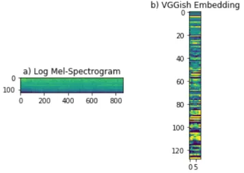
Figure 1: Input features for a sample input file. X-axis is time. a) Log-mel spectrogram: 128 mel bins, 862 time bins. b) VGGish embedding: 128 dimensions, 10 time bins.
3. FEATURE EXTRACTION 3.1. Data augmentation and spectrogram generation
To help the model generalize and to augment the dataset, each file was subjected to pitch shifting, volume changing, and an addition of background noise. After augmentation, each audio file was con-verted into a log-mel spectrogram with 128 mel bins. The original sample rate of 44.1 kHz was retained, resulting in each spectrogram having 862 time bins. The VGGish features (128x10) from the pre-trained AudioSet model were also generated for each input file. See Figure 1 for a visualization.
3.2. Label choice
To assign labels to each example, we tried several configurations that take into account the disagreement among human annotators. We tried several different thresholds of agreement from 25 percent to 75 percent agreement yielding a positive value. We also tried assigning labels as a float that represents the agreement among an-notators. We achieved the best results when we restricted positive labels to only classes that had over 50 percent agreement from peo-ple who voted on that particular class.
4. MODELS
To build our model, we began by feeding log-mel spectrogram val-ues into a VGGish architecture, and then modified the architec-ture parameters based on training results from the Task 5 dataset. The VGGish architecture failed to improve past the first epoch— possibly the model was overfitting due to the large number of lay-ers and the relatively small size of the dataset. By removing some convolutional layers and maxpooling layers, the model would learn more gradually and continue to improve after the first epoch.
In addition to removing layers, we found that altering the ker-nel sizes improved training. Details of the convolution layers are given in Table 1 and Table 2, where each row describes a ”con-volution block” of the following sequence of layers: con”con-volution, maxpool, batch normalization, and dropout. In a given block, some
Figure 2: Hierarchical model.
of the layers may not be present, as specified in those tables. The first convolution block has a kernel size of 1x1, which was bor-rowed from ConvNet configurations, although the 1x1 layers oc-cur in later layers rather than the first in [9]. ForCNN+VGGish1, CNN+VGGish2, both fine- and coarse-level classification mod-els used inHierarchical1, and the coarse-level classification model used inHierarchical2andHierarchical3, the third convolution block features a large and rectangular (16x128) kernel size with a large stride and padding. We modified the configuration for the fine-level classification model used inHierarchical2 andHierarchical3to reduce this to a smaller kernel – Table 2 gives the kernel size, stride, and padding used in those models.
Each convolution block contains batch normalization and dropout at a rate of0.5. One maxpooling layer follows the third
convolution block.
4.1. CNN + VGGish
The results of our CNN model were unable to surpass the baseline results, so we decided to merge the AudioSet-based VGGish em-beddings into our trained model at the fully-connected layer level (see Table 3). The output of our CNN model was 256 channels of 1 value (256x1) while the VGGish embedding output was 128x10. These outputs were flattened (to vectors of length 256 and 1280, respectively) and concatenated to yield a 1536-dimensional vector which was followed by three fully-connected layers that reduce the dimensionality to 512, 256, and finally the desired number of out-put classes. Batch normalization is applied to each fully-connected layer, as is a dropout rate of 0.2. Adding the VGGish embeddings improved our training results and allowed us to surpass the baseline results for some metrics.
4.2. Hierarchical
Because the class labels are given in terms of a known two-level hierarchy, we built an alternative model that takes the label hier-archy into account. Our model is similar to the ”Local classifier per parent node” approach in [8]. A top-level modelMCwas built
that would predict probabilities for each of the eight “coarse” la-bels. Two of the “coarse” labels (non-machinery-impactand dog-barking-whining) only had a single associated “fine” la-bel, so a prediction from the top-level model of one of these two classes was hard-coded to generate the same probability of tion for the associated fine-label class. To handle fine-label predic-tions for sound events in the other coarse categories, six individual low-level models{MFi|COARSE=i},1≤i≤6were trained
to classify the probability for each of the fine labelsi, conditioned on knowledge of the coarse class label for a particular example. This resulted in a total of seven models; see Figure 2. Each of these models had essentially the same structure, with the exception of the number of nodes in the output layer.
the coarse classifierMC(see Section 5). The dataset for each
clas-sifier was generated by simply extracting the subset of training data where the coarse label was that expected for the fine-label classifier. E.g., for the engine classifier, the data used for training consisted of solely those examples where the coarse label was identified in the ground truth asengine.
We constructed a working classification system from these models as follows. First an unknown input example would be given to the coarse-level classifierMC. Then, the coarse category with
the maximum output value would determine which modelMFi to
run to determine the fine label output values. Finally, if any other coarse categories were output with value>0.5, the corresponding
modelsMFi would be run as well to generate additional possible
fine label classifications.
5. TRAINING TECHNIQUES
For CNN+VGGish1, CNN+VGGish2, Hierarchical1, and the coarse-level classification model of Hierarchical2 and Hierarchical3, we used an Adam optimizer [10] with a learn-ing rate of0.001. Regarding the fine-level classification model for
Hierarchical2 and Hierarchical3, we found that using an RMSProp optimizer [11] with a learning rate of0.01performed better. For the loss function, we used binary cross entropy with log-its, which combines the sigmoid function with binary cross entropy. The loss function is defined as:
ln,c=−wn,c[pcyn,c·logf(xn,c)+(1−yn,c)·log(1−f(xn,c))]
(1) wheref(xn,c)∈[0,1]cpredicts the presence probabilities of sound
categories.cis the class number,nis the index of the sample in the
batch, andpis the weight of the positive answer for the classc. We also experimented with modifying the loss function to give weight to classes based on their representation in the dataset. While fully weighting classes to offset the dataset imbalance decreased the micro AUPRC scores, smoothing the weights—such taking the tenth root of each value—helped under-represented classes perform better and made a slight overall improvement to the micro AUPRC scores (results of these experiments not shown here).
When training the coarse-level models, we implemented a mod-ified form of warm restarts[12]. We monitored the micro AUPRC scores of coarse classes on the validation set, and when coarse mi-cro AUPRC scores had not improved by a specified ”stagnation” threshold, the learning rate was reduced. This process was repeated until a minimum learning-rate threshold was reached. The model then would be reset to the original learning rate and made to cycle through again, with the rate of learning ratereductionset to be less severe. We saved a new best model at the end of any epoch that resulted in a new highest micro AUPRC score.
Training of the ”branch” models for fine-grained classification in the threeHierarchicalmodels proceeded differently, with-out warm restarts. For each fine-grained classifier, we reduced the learning rate by multiplying it by a factorγafter a certain number of
epochsp(for ”patience”) passed with no improvement to the loss. For theHierarchical1model we setγ= 0.1andp= 5, while for theHierarchical2andHierarchical3variants we set
γ = 0.2andp= 6. We saved a new best model at the end of any epoch that resulted in a new lowest validation loss.
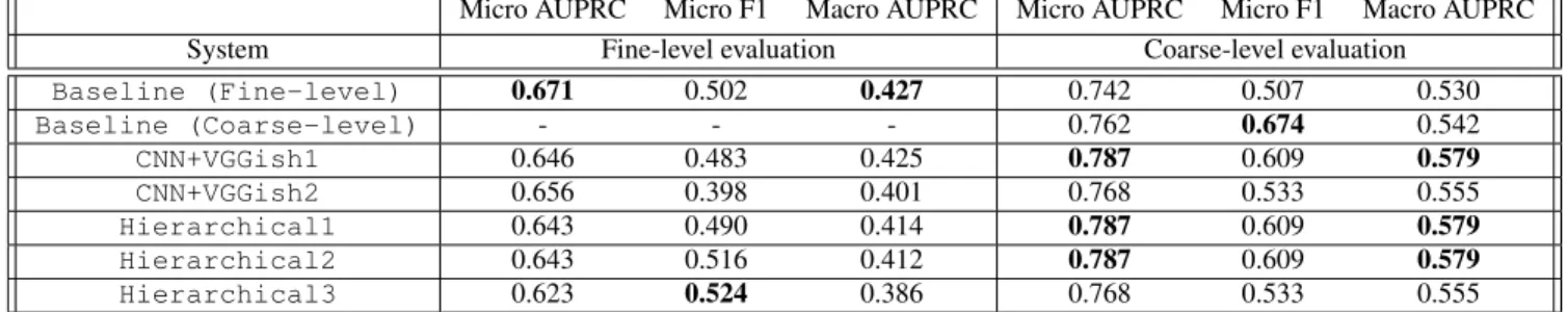
Our results can be found in Table 4. Our method was able to sur-pass the Micro AUPRC and Macro AUPRC baseline scores in the coarse-level evaluation. However, our method was unable to beat the baseline in fine-level evaluation. BothCNN+VGGishmodels are checkpoints from different points of a single training session; the best fine-level score was achieved before the best coarse-level score.
We adopted the CNN+VGGish1 model as the coarse-level classifier for theHierarchical1andHierarchical2 mod-els. For Hierarchical3 the coarse-level classifier was the CNN+VGGish2model. For all theHierarchicalmodels, the results were worse than those of the best single model trained to jointly output fine and coarse labels (CNN+VGGish1), except for one metric: Micro F1 for the fine-level evaluation. Notice that we were able to increase the fine-level Micro F1 score from0.490
(Hierarchical1) to0.524(Hierarchical3) via the modi-fications noted above to the optimization parameters. Notably, the latter score of0.524was better than the baseline system result of 0.502. However, this Micro F1 optimization also lead to a decrease in the Micro AUPRC and Macro AUPRC scores in the fine-level evaluation.
The inferior results of the threeHierarchicalmodels for Micro and Macro AUPRC were a surprise, but they seem to indi-cate that the single model has more than enough parameters to do both fine and coarse tasks simultaneously. A possible explanation is that the fine-level modelsMFiwere only trained on a strict subset
of the dataset. An improvement might be to use the entire dataset, but to assign a new dummy output label in the ground truth for all examples where the coarse label6=i, in order to provide more neg-ative examples.
7. CONCLUSIONS
Our results show how fusing a custom CNN model with VGGish embeddings can impact scores. Furthermore, creating a hierar-chical model has the potential to fine-tune subset classes of indi-vidual coarse classes. Further hyper-parameter tuning may yield better results, as may further experimentation with data augmen-tation. For more details please refer to our GitHub repository at https://github.com/microsoft/dcase-2019.
As future work, we plan to perform segmentation on the time-frequency domain to obtain background and foreground segments and adopt classification models on them to further improve the per-formance.
Conv Block In Channels Out Channels Kernel Size Stride Padding Batch Norm Max Pooling Dropout 1 1 8 (1,1) (1,1) (0,0) True False .5 2 8 16 (3,3) (1,1) (1,1) True False .5 3 16 32 (16,128) (4,16) (8,16) True (4,4) .5 4 32 64 (5,5) (2,2) (1,1) True False .5 5 64 128 (5,5) (2,2) (1,1) True False .5 6 128 256 (3,3) (2,2) (1,1) True False .5
Table 1: Convolution blocks ofCNN+VGGish1,CNN+VGGish2, both fine- and coarse-level classification models inHierarchical1, and the coarse-level classification model used inHierarchical2andHierarchical3.
Conv Block In Channels Out Channels Kernel Size Stride Padding Batch Norm Max Pooling Dropout
1 1 8 (1,1) (2,2) (0,0) True False .5 2 8 16 (3,3) (2,2) (1,1) True False .5 3 16 32 (3,3) (4,4) (1,1) True (4,4) .5 4 32 64 (5,5) (2,2) (1,1) True False .5 5 64 128 (3,3) (3,3) (1,1) True False .5 6 128 256 (3,3) (3,3) (1,1) True False .5
Table 2: Convolution blocks of the fine-level classification model used inHierarchical2andHierarchical3.
FC-Layer In Channels Out Channels Batch Norm Dropout
Bilinear (256,1280) 512 True .2
Linear 512 256 True .2
Linear 256 number of classes False None
Table 3: Combining VGGish embeddings with spectrogram convolution output in fully-connected layers.
Micro AUPRC Micro F1 Macro AUPRC Micro AUPRC Micro F1 Macro AUPRC System Fine-level evaluation Coarse-level evaluation
Baseline (Fine-level) 0.671 0.502 0.427 0.742 0.507 0.530 Baseline (Coarse-level) - - - 0.762 0.674 0.542 CNN+VGGish1 0.646 0.483 0.425 0.787 0.609 0.579 CNN+VGGish2 0.656 0.398 0.401 0.768 0.533 0.555 Hierarchical1 0.643 0.490 0.414 0.787 0.609 0.579 Hierarchical2 0.643 0.516 0.412 0.787 0.609 0.579 Hierarchical3 0.623 0.524 0.386 0.768 0.533 0.555 Table 4: Results: metrics computed on validation set. Best results for each metric indicated inbold.
[1] M. Thorogood, J. Fan, and P. Pasquier, “Soundscape audio signal classification and segmentation using listeners percep-tion of background and foreground sound,”Journal of the Au-dio Engineering Society, vol. 64, no. 7/8, pp. 484–492, 2016. [2] D. Conte, P. Foggia, G. Percannella, A. Saggese, and
M. Vento, “An ensemble of rejecting classifiers for anomaly detection of audio events,” pp. 76–81, 2012.
[3] A. Farina and P. Salutari, “Applying the ecoacoustic event detection and identification (EEDI) model to the analysis of acoustic complexity,” vol. 14, pp. 13–42, 2016.
[4] P. J. Bello, C. Silva, O. Nov, R. L. Dubois, A. Arora, J. Sala-mon, C. Mydlarz, and H. Doraiswamy, “Sonyc: A system for monitoring, analyzing, and mitigating urban noise pollution,”
Communications of the ACM, vol. 62, no. 2, pp. 68–77, 2019. [5] S. Hershey, S. Chaudhuri, D. P. W. Ellis, J. F. Gemmeke, A. Jansen, C. Moore, M. Plakal, D. Platt, R. A. Saurous, B. Seybold, M. Slaney, R. Weiss, and K. Wilson, “CNN architectures for large-scale audio classification,”
in International Conference on Acoustics, Speech and
Signal Processing (ICASSP), 2017. [Online]. Available: https://arxiv.org/abs/1609.09430
[6] R. F. Lyon,Human and Machine Hearing: Extracting Mean-ing from Sound. Cambridge University Press, 2017. [7] N. Takahashi, M. Gygli, B. Pfister, and L. V. Gool, “Deep
convolutional neural networks and data augmentation for acoustic event detection,”CoRR, vol. abs/1604.07160, 2016. [Online]. Available: http://arxiv.org/abs/1604.07160
[8] C. N. Silla and A. A. Freitas, “A survey of hierarchical classification across different application domains,” Data
Mining and Knowledge Discovery, vol. 22, no. 1, pp.
31–72, Jan 2011. [Online]. Available: https://doi.org/10.1007/ s10618-010-0175-9
[9] K. Simonyan and A. Zisserman, “Very deep convolutional networks for large-scale image recognition,” arXiv preprint arXiv:1409.1556, 2014.
[10] D. P. Kingma and J. Ba, “Adam: A method for stochastic op-timization,”arXiv preprint arXiv:1412.6980, 2014.
[11] T. Tieleman and G. Hinton, “Rmsprop, coursera: Neural net-works for machine learning,”Technical report, 2012. [12] I. Loshchilov and F. Hutter, “SGDR: Stochastic gradient
de-scent with warm restarts,”arXiv preprint arXiv:1608.03983, 2016.