An Improved Method for Bandwidth Selection when Estimating ROC Curves

(1)

ISSN 1440-771X

AUSTRALIA

DEPARTMENT OF ECONOMETRICS

AND BUSINESS STATISTICS

An Improved Method for Bandwidth Selection

When Estimating ROC Curves

Peter G Hall and Rob J Hyndman

(2)

when estimating ROC curves

Peter G. Hall1 and Rob J. Hyndman1,2 13 September 2002

Abstract: The receiver operating characteristic (ROC) curve is used to describe the performance of a diagnostic test which classifies observations into two groups. We introduce a new method for selecting bandwidths when computing kernel estimates of ROC curves. Our technique allows for interaction between the distributions of each group of observations and gives substantial improvement in MISE over other proposed methods, especially when the two distributions are very different.

Key words: Bandwidth selection; binary classification; kernel estimator; ROC curve.

JEL classification: C12, C13, C14.

1 INTRODUCTION

A receiver operating characteristic (ROC) curve can be used to describe the performance of a diagnostic test which classifies individuals into either group G1 or group G2. For example, G1 may contain individuals with a disease and G2 those without the disease. We assume that the diagnostic test is based on a continuous measurement T and that a person is classified as G1 if T ≥ τ and G2 otherwise. Let G(t) = Pr(T ≤ t | G1) and

F(t) = Pr(T ≤t|G2) denote the distribution functions ofT for each group. (Thus F is the specificity of the test and 1−G is the sensitivity of the test.) Then the ROC curve is defined as R(p) = 1−G(F−1₍₁₋_p_{)) where 0}_≤_p_≤_1.

Let{X1, . . . , Xm}and{Y1, . . . , Yn}denote independent samples of independent data

from G1 and G2, and let ˆF and ˆG denote their empirical distribution functions. Then a simple estimator of R(p) is ˆR(p) = 1−Gˆ( ˆF−1₍₁₋_p_{)), although this has the obvious} weakness of being a step function while R(p) is smooth.

Zou, W.J. Hall & Shapiro (1997) and Lloyd (1998) proposed a smooth kernel estimator of R(p) as follows. Let K(x) be a continuous density function andL(x) = R_−∞x K(u)du. The kernel estimators of F and Gare

e F(t) = 1 m m X i=1 L _t₋_X i h1 and Ge(t) = 1 m m X i=1 L _t₋_Y i h2 .

1_{Centre for Mathematics and its Applications, Australian National University, Canberra ACT 0200,}

Australia.

2_{Department of Econometrics and Business Statistics, Monash University, VIC 3800, Australia.}

(3)

An improved method for bandwidth selection when estimating ROC curves

For the sake of simplicity we have used the same kernel for each distribution, although of course this is not strictly necessary. The kernel estimator of R(p) is then

e

R(p) = 1−Ge(Fe−1(1−p)).

Qiu & Le (2001) and Peng & Zhou (2002) have discussed estimators alternative to Re(p). Lloyd and Yong (1999) were the first to suggest empirical methods for choosing band-widths h1 and h2 of appropriate size for Re(p), but they treated the problem as one of estimating F and Gseparately, rather than of estimating the ROC function R. We shall show that by adopting the latter approach one can significantly reduce the surplus of mean squared error over its theoretically minimum level. This is particularly true in the practi-cally interesting case whereF andGare quite different. In the present paper we introduce and describe a bandwidth choice method which achieves these levels of performance.

A related problem, which leads to bandwidths of the correct order but without the correct constants, is that of smoothing in distribution estimation. See, for example, Miel-niczuk, Sarda and Vieu (1989), Sarda (1993), Altman and Leg´er (1995), and Bowman, Hall and Prvan (1998).

2 METHODOLOGY

2.1 Optimality criterion and optimal bandwidths

If the tails of the distribution F are much lighter than those of G then the error of an estimator of F in its tail can produce a relatively large contribution to the error of the corresponding estimator of G(F−1_{). As a result, if the}_L2 _{performance criterion}

α1(S) =

Z S

EhGb(Fb−1(p))−G(F−1(p))i2 dp (2.1)

for a set S ⊆ [0,1], is not weighted in an appropriate way then choice of the optimal bandwidth in terms ofα1(S) can be driven by relative tail properties of f andg. Formula (A.1) in the appendix will provide a theoretical illustration of this phenomenon. We suggest that the weight be chosen equal tof(F−1), so that the L2 criterion becomes

α(S) =

Z S

EhGb(Fb−1(p))−G(F−1(p))i2f(F−1(p))dp . (2.2)

We shall show in the appendix that for this definition of mean integrated squared error, α(S)∼β(S)≡ Z F−1(S) n E[Fb(t)−F(t)]2g2(t) + E[Gb(t)−G(t)]2f2(t)odt (2.3)

where F−1(S) denotes the set of points F−1(p) with p ∈ S. Note particularly that the right-hand side is additive in the mean squared errors E(Fb−F)2 and E(Gb−G)2, so that in principleh1andh2 may be chosen individually, rather than together. That is, ifh1 and

(4)

h2 minimise β1(S) = Z F−1(S) E[Fb(t)−F(t)]2g2(t)dt and β2(S) = Z F−1(S) E[Gb(t)−G(t)]2f2(t)dt,

respectively, then they provide asymptotic minimisation of α(S).

To express optimality we take F−1₍_S_{) equal to the whole real line, obtaining the} global criterion γ(h1, h2) =γ1(h1, h2) +γ2(h1, h2) where

γ1(h1, h2) = Z ∞ −∞ E[Fb(t)−F(t)]2g2(t)dt and γ2(h1, h2) = Z ∞ −∞ E[Gb(t)−G(t)]2f2(t)dt (2.4) Suppose K is a compactly supported and symmetric probability density, and f0 is bounded, continuous and square-integrable. Then arguments similar to those of Azzalini (1981) show that

E(Fb−F)2 =m−1[(1−F)F −h1κ f] + (1₂κ2h21f0)2+o(n−1h1+h41),

whereκ=R(1−L(u))L(u)du, κ2 =R u2K(u)du. Of course, an analogous formula holds for E(Gb−G)2, and so the formulae at (2.4) admit simple asymptotic approximations:

γ1 = m−1 Z (1−F)F g2+δ1+o(m−1h1+h41) γ2 = n−1 Z (1−G)G f2+δ2+o(n−1h2+h42) where δ1 = −m−1h1κ Z f g2+1₄κ2₂h4₁ Z (f0g)2 (2.5) and δ2 = −n−1h2κ Z f2g+1₄κ2₂h4₂ Z (f g0)2 (2.6)

The asymptotically optimal bandwidths are therefore

h1=m−1/3c(f, g) and h2 =n−1/3c(g, f) where c(f, g)3 = κ Z f(u)g2(u)du κ2₂ Z [f0(u)g(u)]2du .

A conventional plug-in rule for choosing h1 and h2 may be developed directly from these formulae. However, it requires selection of pilot bandwidths for estimatingf, gand their derivatives. The technique suggested in the next section avoids that difficulty.

(5)

2.2 Empirical choice of bandwidth

Let cf2 _and c_g2 _{denote leave-one-out kernel estimators of}_f2 _and _g2_{, respectively:}

c f2₍_x_|_h 1) = 2 m(m−1)h2 1 X X 1≤i1<i2≤m Kx−Xi1 h1 Kx−Xi2 h1 c g2₍_y_|_h 2) = 2 n(n−1)h2 2 X X 1≤i1<i2≤n Ky−Yi1 h2 Ky−Yi2 h2 .

Let ˆf−i(x|h1) ={(m−1)h1}−1 Pj=6 i K{(x−Xj)/h1}, and define ˆg−i(y|h2) analogously, and let fc2

1 and cg21 denote the kernel estimators of (f0)2 and (g0)2, respectively:

c f₁2(x|h1) = 2 m(m−1)h4 1 m X i1=1 m X i2=1 K0x−Xi1 h1 K0x−Xi2 h1 c g₁2(y|h2) = 2 n(n−1)h4 2 n X i1=1 n X i2=1 K0y−Yi1 h2 K0y−Yi2 h2 .

Note that the latter two estimators include all terms whereas the other estimators are “leave-one-out” estimators. We include the diagonal terms in the estimators of (f0₎2 _and (g0)2 as they act like ridge parameters and produce better empirical performance.

We could choose h1 and h2 to minimize ∆(h1, h2). To motivate this approach, note that

E{∆(h1, h2)} = −m−1h1κ Z (Eˆg)2f +1₄κ2₂h4₁ Z (E ˆf0)2(Eˆg)g −n−1h2κ Z (E ˆf)2g+1₄κ2₂h4₂ Z (Eˆg0)2(E ˆf)f , (2.7) which indicates that ∆ is an almost-unbiased approximation to δ = δ1 +δ2; compare (2.7) with the sum of the terms at (2.5) and (2.6). The relative size of stochastic error may also be shown to be asymptotically negligible. Indeed, if m n asn → ∞, if K is compactly supported and has a H¨older-continuous derivative, and iff andgare compactly supported and have three bounded derivatives, then ∆(h1, h2)/δ(h1, h2) converges to 1 with probability 1, uniformly in n−1+_≤_h

1, h2 ≤n− for each 0< < 1₂, asn→ ∞. However, minimizing ∆(h1, h2) leads to some numerical instability. Instead, we con-strain the minimization so that h1 = ρh2 whereρ =h∗1/h∗2 and h∗1 and h∗2 are the band-widths selected for estimatingF andGusing the plug-in rule proposed by Lloyd and Yong (1999). Minimizing ∆(h1, h2) under this constraint provides values ofh1 andh2 which are suitable for estimating Re(p).

(6)

3 SOME SIMULATIONS

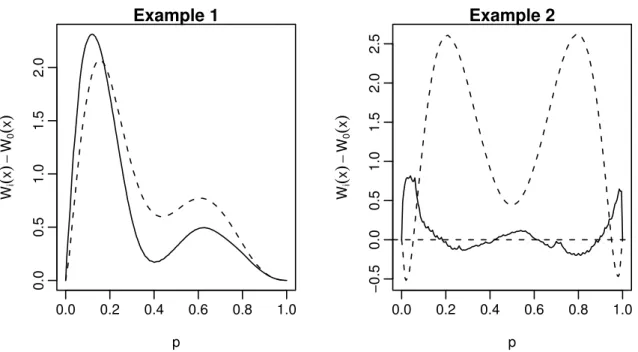
We compare the estimates obtained with our bandwidth selection method outlined above to those obtained by Lloyd and Yong (1999) using their plug-in rule. Let

W(p) =EhGe(Fe−1(p))−G(F−1(p))i2 f(F−1(p)) (3.1) denote mean squared error. Thus, mean integrated squared error, introduced at (2.2), is given by α(S) = R_SW(p)dp. The ideal but practically unattainable minimum of W(p), for a nonrandom bandwidth, can be deduced by simulation, and will be denoted byW0(p). This value will be compared with its analogue,W1(p), obtained from (3.1) using the values of h1 and h2 chosen using the method outlined in Section 2.2; and withW2(p), obtained from (3.1) using the values of h1 and h2 chosen using the plug-in procedure suggested by Lloyd and Yong (1995).

In our first example, illustrated in the first panel of Figure 1, we used Lloyd and Yong’s (1999) model, where F andGare N(0,1) and N(1,1) respectively. In the second example we chose F and G to be more different; F was N(0,1) and G was an equal mixture of N(−2,1) and N(2,1). In both cases our method offers an improvement, which as expected is greater when the distributions are further apart. The areas under the curves represent the increase inα(S) due to bandwidth selection. In these terms our method improves on that of Lloyd and Yong (1999) by 1.2% and 28.6%, in the respective examples.

0.0 0.2 0.4 0.6 0.8 1.0 0.0 0.5 1.0 1.5 2.0 Example 1 p Wi ( x ) − W0 ( x ) 0.0 0.2 0.4 0.6 0.8 1.0 −0.5 0.0 0.5 1.0 1.5 2.0 2.5 Example 2 p Wi ( x ) − W0 ( x )

(7)

APPENDIX: Derivation of

(2

.

3)

Assume thatf andghave continuous derivatives and are bounded away from 0 onS. Put

A=Fb−F, B =Gb−GandC =Fb−1−F−1, and writeI for the identity function. Then by Taylor expansion,

I =Fb(F−1+C) =I+A(F−1) +C f(F−1) +op(|A(F−1)|+|C|),

whence it follows that C=−[A(F−1₎_/f₍_F−1_{)] +}_o

p(|A(F−1)|). Hence, b G(Fb−1)−G(F−1) = B(F−1)−g(F −1₎ f(F−1₎A(F −1_{) +}_o p(|A(F−1)|+|B(F−1)|). (A.1)

Note the ratio g(F−1₎_/f₍_F−1_{) on the right-hand side of (A.1). Since the variance of}

A equals (1 −F)F then the unweighted criterion α1, defined at (2.1), can be largely determined by the value of (g/f)2(1−F)F in the tails if this quantity is not bounded.

Using instead the weighted criterion α, defined at (2.2), we may deduce from (A.1), related computations and the independence of the samples that

Z S E[Gb(Fb−1)−G(F−1)]2f(F−1) = [1 +o(1)] Z F−1(S) [E(B2)f2+ E(A2)g2] which is equivalent to (2.3).

REFERENCES

Altman, N. and L´eger, C. (1995). Bandwidth selection for kernel distribution function

estimation. J. Statist. Plann. Inf.46, 195–214.

Azzalini, A. (1981). A note on the estimation of a distribution function and quantiles

by a kernel method.Biometrika 68, 326–328.

Bowman, A.W., Hall, P. and Prvan, T. (1998). Cross-validation for the smoothing

of distribution functions. Biometrika85, 799–808.

Lloyd, C.J. (1998). The use of smoothed ROC curves to summarise and compare

diag-nostic systems.J. Amer. Statist. Assoc. 93, 1356–1364.

Lloyd, C.J. and Yong, Z(1999). Kernel estimators of the ROC curve are better than

empirical.Statist. Prob. Letters 44, 221–228.

Mielniczuk, J., Sarda, P. and Vieu, P. (1989). Local data-driven bandwidth choice

for density estimation. J. Statist. Plann. Inf.23, 53–69.

Peng, L. and Zhou, X.-H. (2002). Local linear smoothing of receiver operator

charac-teristic (ROC) curves.J. Statist. Plann. Inf., to appear.

Qiu, P. and Le, C. (2001). ROC curve estimation based on local smoothing.J. Statist.

Comput. and Simul.70, 55–69.

Sarda, P. (1993). Smoothing parameter selection for smooth distribution functions. J.

Statist. Plann. Inf.35, 65–75.

Zou, K.H., Hall, W.J. and Shapiro, D.E. (1997). Smooth non-parametric receiver

operating characteristic (ROC) curves for continuous diagnostic tests. Statistics in Medicine 162143–2156.