Air Force Institute of Technology
AFIT Scholar
Theses and Dissertations Student Graduate Works
3-21-2013
Learning Enterprise Malware Triage from
Automatic Dynamic Analysis
Jonathan S. Bristow
Follow this and additional works at:https://scholar.afit.edu/etd
Part of theDigital Communications and Networking Commons, and theElectrical and Computer Engineering Commons
This Thesis is brought to you for free and open access by the Student Graduate Works at AFIT Scholar. It has been accepted for inclusion in Theses and Dissertations by an authorized administrator of AFIT Scholar. For more information, please [email protected].
Recommended Citation
Bristow, Jonathan S., "Learning Enterprise Malware Triage from Automatic Dynamic Analysis" (2013).Theses and Dissertations. 856.
LEARNING ENTERPRISE MALWARE TRIAGE FROM AUTOMATIC DYNAMIC ANALYSIS
THESIS
Jonathan S. Bristow, Captain, USAF AFIT-ENG-13-M-10
DEPARTMENT OF THE AIR FORCE AIR UNIVERSITY
AIR FORCE INSTITUTE OF TECHNOLOGY
Wright-Patterson Air Force Base, Ohio
DISTRIBUTION STATEMENT A.
The views expressed in this thesis are those of the author and do not reflect the official policy or position of the United States Air Force, the Department of Defense, or the United States Government.
This material is declared a work of the U.S. Government and is not subject to copyright protection in the United States.
AFIT-ENG-13-M-10
LEARNING ENTERPRISE MALWARE TRIAGE FROM AUTOMATIC DYNAMIC ANALYSIS
THESIS
Presented to the Faculty
Department of Electrical and Computer Engineering Graduate School of Engineering and Management
Air Force Insitute of Technology Air University
Air Education and Training Command in Partial Fulfillment of the Requirements for the Degree of Master of Science in Computer Science
Jonathan S. Bristow, B.S. Captain, USAF
March 2013
DISTRIBUTION STATEMENT A.
AFIT-ENG-13-M-10
Abstract
Adversaries employ malware against victims of cyber espionage with the intent of gaining unauthorized access to information. To that end, malware authors intentionally attempt to evade defensive countermeasures based on static methods. This thesis analyzes a dynamic analysis methodology for malware triage that applies at the enterprise scale.
This study captures behavior reports from 64,987 samples of malware randomly selected from a large collection and 25,591 clean executable files from operating system install media. Function call information in sequences of behavior generate feature vectors from behavior reports from the files. The results of 64 experiment combinations indicate that using more informed behavior features yields better performing models with this data set. The decision tree classifier attained a max performance of 0.999 area under the ROC curve and 99.4% accuracy using argument information with function sequence lengths from 11–14.
This methodology contributes to strategic cyber situation awareness by fusion with fast malware detection methods, such as static analysis, to change the game of malware triage in favor of cyber defense. This method of triage reduces the number of false alarms from automatic analysis that allows a 97% workload reduction over using a static method alone.
Dedicated to our Lord, to my wife and our children, to my mother, to dear friends, to liberty, and to the United States of America
Acknowledgments
Thank you, Jesus Christ, my Lord and Savior, for freely justifying me through faith in your atoning blood. You give me peace through seemingly trying times despite my myriad personal failures.
Thank you, my beautiful, loving bride. Your help exactly meets my needs, and you are a true blessing in my life. I also thank you for your sacrifices and overcoming in bringing our (currently) four children into this world, and for teaching and training them to walk in truth.
Thank you, mother, for always encouraging me academically. Your sacrifices have made this journey and these opportunities possible.
Thank you, Major Thomas Dube, PhD, my wise academic advisor. Your vision and advice inspires me. Thank you also to the members of my thesis committee. Your rigor has taught me a great deal about conducting research.
Also thank you to my fellow students and to the faculty and staff of the Air Force
Institute of Technology.
Ultimately, thank you to the courageous people who have put their lives on the line in war and vigilance; striving for love of liberty so that we may enjoy the blessing of freedom from tyranny and usurpation in this blessed nation.
Table of Contents
Page
Abstract . . . iv
Dedication . . . v
Acknowledgments . . . vi
Table of Contents . . . vii
List of Figures . . . ix
List of Tables . . . x
List of Acronyms . . . xi
I. Introduction . . . 1
II. Literature Review . . . 4
2.1 Machine Learning . . . 4
2.2 Static Analysis . . . 6
2.3 Dynamic Analysis . . . 7
2.3.1 API Call Sequences . . . 9
2.3.2 Behavior Analysis . . . 12
2.4 Summary . . . 14
III. Methodology . . . 17
3.1 Problem Definition . . . 17
3.1.1 Goals and Hypothesis . . . 17
3.1.2 Approach . . . 18 3.2 System Boundaries . . . 18 3.3 System Services . . . 19 3.4 Workload . . . 21 3.5 Performance Metrics . . . 22 3.6 System Parameters . . . 23
3.6.1 Dynamic Analysis Engine . . . 23
3.6.2 Feature Generation Component . . . 25
Page
3.7 Factors . . . 26
3.8 Evaluation Technique . . . 27
3.9 Experimental Design . . . 27
3.10 Methodology Summary . . . 27
IV. Results and Analysis . . . 28
4.1 Feature Generation and Selection . . . 28
4.2 Classifier Performance . . . 31
4.2.1 Overview . . . 31
4.2.2 Normalization . . . 31
4.2.3 MIST andqDetails . . . 32
4.3 Number of Samples . . . 33
4.4 Timing Analysis . . . 37
4.5 Operational Analysis . . . 38
4.6 Limitations Analysis . . . 43
4.6.1 Malware Set Limitations . . . 43
4.6.2 Dynamic Analysis Limitations . . . 43
V. Conclusions . . . 45
5.1 Research Conclusions . . . 45
5.2 Research Significance . . . 46
5.3 Future Work Recommendations . . . 48
5.3.1 Data Set Issues . . . 48
5.3.2 Machine Learning Algorithms . . . 49
5.3.3 Feature Selection . . . 49
Appendix A: Top 10 Performance Results . . . 51
Appendix B: Experiment Result Details . . . 55
List of Figures
Figure Page
2.1 An example of a 2-gram at MIST level 1 . . . 10
2.2 An example of a 1-gram at MIST level 2 . . . 11
3.1 Malware Detection System Component Diagram . . . 19
4.1 Number of q-grams Present by Factors . . . 30
4.2 Details and chart of area under ROC comparisons of classifier performance . . 32
4.3 Comparison of MIST levels andq-gram lengths . . . 33
4.4 Comparison of resulting sample sizes by MIST level and gram length . . . 34
4.5 Performance according to resulting sample size . . . 35
List of Tables
Table Page
2.1 Overview summary of related work . . . 15
2.2 Detailed summary of related work . . . 16
3.1 Factor Levels . . . 26
4.1 Summary of dynamic analysis performance . . . 28
4.2 Detailed examples of feature generation component results . . . 29
4.3 Detailed examples of feature selection rates . . . 36
4.4 Top 10 Data Sets by False Positive Rate (FPR) . . . 40
A.1 Top 10 Data Sets by Classifier Performance according to the Area under ROC (AUC) . . . 51
A.2 Top 10 Data Sets by Classifier Performance according to the Percent Correct . . 52
A.3 Significance of MIST Level by Factor Levels . . . 53
A.4 Significance of Normalization by Factor Levels . . . 54
B.1 Experiment Result Details for MIST level 1 . . . 56
B.2 Experiment Result Details for MIST level 1, continued . . . 57
B.3 Experiment Result Details for MIST level 2 . . . 58
List of Acronyms
Acronym Definition
API application programming interface
AUC area under the receiver operating characteristic (ROC) curve
CFG control flow graph
CUT Component under Test
DLL dynamic link library
ECI enterprise cyber infrastructure
HCL hierarchical clustering with complete linkage
kNN k-nearest-neighbors
LSH locality-sensitive hashing
MaTR malware target recognition
MIST malware instruction set
MLP multilayer perceptron
NB na¨ıve Bayes
ROC receiver operating characteristic
SUT System under Test
SVM support vector machine
LEARNING ENTERPRISE MALWARE TRIAGE FROM AUTOMATIC DYNAMIC ANALYSIS
I. Introduction
M
alware plagues enterprise networks. Malware authors intentionally attempt toevade defensive countermeasures. These adversaries employ malware against victims of cyber espionage with the intent of gaining unauthorized access to information or performing other malicious behavior such as corrupting data or denying access to information. As long as it is possible to use malware to achieve gain, then adversaries will attempt to introduce malware into enterprise cyber infrastructures (ECIs) [15].
Cyber defenders deploy a variety of responses to mitigate the threat of malware.
To counteract signature-based malware detection, such as antivirus products and static
analysis, malware authors implement a variety of obfuscation techniques that change the digital “appearance” of malware while preserving malicious behavior [9, 28, 31].
Initial results indicate that a dynamic analysisof malware can reveal malware hidden to
static analysis by intentional obfuscation by observing the actual behavior of executable
files [21, 26]. Furthermore, a dynamic analysis approach is significantly different from a
static analysis approach such that one can refine the results of the other. That is, applying a dynamic method to the results of a previous static method can reduce the false alarms of
both methods together for a more efficient malware detection system [6].
Manual review of large sets of dynamic analysis reports remains unfeasible because
an enterprise network contains hundreds of thousands of unique executable files. Malware
triage seeks to reduce the workload of the available cyber analysts by detecting the files that most closely resemble malware.
A given ECI contains executable files from a variety of sources. Operating systems install some executable files at install time or during updates, and others reside as part of an application that provides some set of features. Some applications directly support the requirements of the users of the ECI, while other applications provide a variety of security services, such as antivirus software, anti-spyware software or host-based intrusion detection system software. Another source of executable files on ECIs is administrative programs such as application installers or remote management software. Each application contains a set of executable files that interact together to provide the service of the application. Thus, each executable file behaves in a certain way, and there are a large variety of acceptable behaviors present from executable files on a typical ECI.
Additionally, some ECIs contain malicious executable files that provide a service to unauthorized users. Adversaries specifically program such executable files to perform malicious behaviors and covertly introduce them to the ECI. Examples include remote control of resources, information stealing or destructive actions. Cyber defenders must detect and remove these malicious executables in order to continue to meet the mission requirements of the enterprise.
This thesis examines the effects of feature extraction and selection on enterprise-level malware triage, and provides a methodology for behavioral analysis of unknown executable files with the goal of detecting malicious executables. Furthermore, this methodology contributes to strategic cyber situation awareness by combining with fast malware detection methods, such as static analysis, to change the game of malware triage in favor of cyber defense.
Analysis of the experiments validates using both application programming interface (API) argument information and behavior sequences of lengths from 11–14 to build more accurate executable classification models, and does not find a significant benefit of normalization. Given the high accuracy of 99.4% correct and low false positive rate
of 1.75%, this method presents a prime candidate for a middle level dynamic method in a malware target recognition (MaTR) architecture [7].
Following is a summary of contributions of this thesis:
• critical analysis of recent automatic malware analysis research including a
compari-son to this study (Sections 2.3.2 and 2.4),
• analysis and discussion of results from 64 experiments on 3 key parameters of
behavior analysis feature generation that the literature does not cover in a detailed manner (Chapter 4), and
• analysis of the contribution to a malware target recognition architecture by this
dynamic analysis method, which establishes the feasibility of automatic behavior analysis at the enterprise scale (Sections 4.5 and 5.2).
This thesis covers a number of considerations for cyber defenders to prudently design a malware detection system, including the following summary. Cyber defenders using a malware detection system must:
• match the analysis sandbox environment to the enterprise environment,
• tailor the training set to the types of threats that face the particular enterprise,
• select features to represent the unique behaviors of benign and malicious programs,
• use an efficient dynamic analysis component,
• experiment with around eight levels of parameters when retraining,
• keep the number of training validation repetitions less than 10 (e.g. use 3 or 1),
• analyze the independence of the methods in different MaTR tiers, and
II. Literature Review
T
hischapter introduces the background of machine learning (Section 2.1) and malwareanalysis (Section 2.2) before surveying recent research in dynamic analysis and automatic behavior classification (Section 2.3).
2.1 Machine Learning
The field of Machine learning involves using theories of statistics, algorithms, and
knowledge representation to automatically represent information in a digitalmodelof the
real world. The classificationprocess involves building a model on two or more distinct
classes of training samples, and the model then attempts to predict the class of test samples. Decision trees build a classification model by repeatedly bisecting the input space based on a single attribute at a time. The tree building algorithm chooses the attribute that is most likely to evenly cut the space by measuring the information gain of all the available attributes according to the class labels. The support vector machine (SVM) algorithm finds a nonlinear classification boundary by selecting training samples that minimize the distance to the boundary [8]. The Wakaito Environment for Knowledge Acquisition (WEKA) platform provides implementations of many machine learning algorithms including J48, which implements the C4.5 decision tree algorithm [13, 24, 32].
Where classification uses training data that comes with class labels, clusteringdoes
not need to start with labels in order to put samples into groups. With clustering, a selected similarity measure (based on what makes sense for the data set) determines the relative distance between samples. Then the chosen algorithm dictates how the measurements shall
determine which samples belong together in clusters. The hierarchical clustering with
complete linkage (HCL) method finds the shortest distance between two existing clusters then combines the clusters by linking one sample from each cluster that maximizes the
distance between those two samples. After repeating that algorithm until all the samples link to a single cluster a provided threshold cuts the resulting tree relationship into a set of clusters that each have a height that is no greater than the threshold [32].
Other learning algorithms, weak learners, perform only slightly better than random
guessing (accuracy slightly above 50% correct for a two-class problem). Ensembles of
weak learners combine many weak learners, each learning a different part of a problem
to create a better-performing model [17]. Weak learners are fast to develop and execute,
but some developers exert more research effort into developing a learning algorithm with
moreheuristics, which means they apply domain knowledge to solving part of the problem ahead of time. The resulting models perform better than weak learners, although more complicated learners necessarily have a higher computational cost [33].
In this effort, pilot studies show that decision trees perform better than bagging or
boosting decision stumps and similarly to bagging or boosting decision trees. Ensembles of decision stumps train more quickly than decision trees, but decision trees train faster than ensembles of decision trees because each ensemble trains 10 models internally.
The practice of k-fold cross validation for building a robust classification model
involves randomly splitting the training sample set into k equally-sizedfolds of samples.
Then the learning algorithm builds a model with a training set of (k−1) folds, leaving one
fold out. Then the algorithm uses the left-out fold as a testing set. Since the algorithm does not train the model with any samples from the test set during an iteration, the unknown
samples validly measure the generality of the model. This process repeats k times, and
each fold becomes the test set for one iteration. Stratified cross validation maintains class
distributions throughout the method so that the relative size of the classes persists through different folds.
2.2 Static Analysis
A static analysis process reveals some attributes of an executable file without executing the code. As a result, the process quickly provides moderate detail. Egele et al. discuss various techniques for automatically analyzing malware and tools that
implement such techniques [9]. Static analysis suffers from generic vulnerabilities
to obfuscation by targeted malware. Moser et al. shows an approach for program
transformation that defeats static analysis methods [21].
Eskandari and Hashemi combine a control flow graph (CFG) from disassembly information with an application programming interface (API) set to attain 97.77% accuracy on a set of 2,140 benign files from Microsoft Windows XP SP3 and 2,305 “network worms” from a repository at Shiraz University [10]. A CFG represents the possible actions that the program could take upon execution. They compare the 97.77% from CFG analysis
to 92.19% accuracy using staticn-grams as features. Both experiments use random forests
on the same sample set. To get around the high processing time from the large graphs of CFG analysis, they flatten each graph into a feature vector using a sparse matrix representation. Disassembly-based information obtains fine-grained information, but it remains vulnerable to obfuscation. The paper does not report how much time the method takes for collection or analysis.
T.E. Dube attains 99.92% detection accuracy on a set of 31,193 samples of 32-bit malware from VX Heavens and 25,195 benign files from a clean install of Microsoft
Windows from vendor media [7]. In comparison with the Kolter and Maloof n-gram
method, Dube’s malware target recognition (MaTR) static method performs significantly more accurately at the 95% confidence level [16]. In his experiments, the best commercial antivirus product fails to achieve 50% accuracy on an unknown malware set. In addition, Dube’s static method averages less than one second of scan time for each file, whereas even the fastest antivirus product tested takes 43 seconds on average. Dube attains this result by
deriving the feature set from proven static features using expert domain knowledge instead
of the computationally heavyn-gram method.
Furthermore, Dube proposes a tiered architecture for cyber situation awareness [6]. In order to triage large amounts of unknown executable files, the bottom tier uses very fast methods that achieve a low false negative rate. When the bottom tier flags a sample as potentially malicious then the sample becomes an input to methods in the middle tier. The middle tier methods still have high detection rates, but also have low false positive rates, because the results from those methods go to cyber analysts at the top tier. Any false positives that reach the top tier are wasted overhead for the analysts, so the false positive rates of the underlying methods provide a way to directly measure the expected waste from overhead. This thesis (Section 5.2) provides insight into a behavior analysis method that fits into the middle tier of such an architecture to improve response times of cyber defenders by reducing the workload.
2.3 Dynamic Analysis
An appropriate dynamic analysis of an executable file reveals the most definitive
information about its actions. Rossow et al. suggest some standard practices for malware experiment design such as removing benign programs from malware collections and commenting on the containment of the samples [27]. Bayer et al. introduce TTAnalyze (now Anubis, which also analyzes Android APK files), which uses Qemu emulation with Windows XP [4, 5]. TTAnalyze successfully reproduces and captures detailed data about the behavior of the executable file under analysis. TTAnalyze collects data at the level of the
emulated processor, but it bridges thesemantic gapwith a kernel driver that leverages the
CR3register and a userland process inside the guest. This means that the analysis method
is able to obtain information about the state of the operating system to allow the process to correctly interpret the low-level instructions.
Yin et al. employ a whole system fine-grained dynamic taint analysis in Panorama [34]. Taint tracking labels the memory address to where a function returns a value, then records when another function uses that value as input or changes the value by writing into the same location again. This tracking allows a low-level emulator to gain insight into how programs interact with the operating system and produce a behavior report for the sand-box system. It collects information from an emulator on the entire guest system including high-level API calls and operating system interaction as well as an instruction trace with taint tracking. The system includes automated user actions during analysis such as typing text and browsing URLs. Upon testing with 42 malware samples and 56 benign samples, Panorama detects all the malware and only reports 3 false positives.
Egele et al. survey the literature on dynamic analysis techniques, tools, and analysis, but do not cover Cuckoo Sandbox, Windows 7 guests or 64-bit guests [9]. When a dynamic system analyzes an unknown executable file, the system may be able to choose which guest system is appropriate. If a malware author targets Windows 7, then the malware may not behave the same if the analysis system executes the file in Windows XP because of API
differences between the versions. A similar phenomenon occurs with 64-bit malware on
a 32-bit analysis system.
Moser et al. explores multiple execution paths during dynamic analysis by taking note of branching points and keeping track of the current state of execution [20]. Building on Anubis, Moser completes one iteration of execution, then reverts back to one of the
branching points to continue analysis down a different path. This method can theoretically
find behaviors of a sample that may not surface otherwise, such as behaviors that require user input or that wait for a specific time. However such completeness comes at the cost
of computation time according the inherentbranching factorof the program, which is how
Lindorfer et al. attempt toDisarmmalware that evades dynamic analysis [18]. Disarm
works by submitting the samples to four different sandboxes and comparing the behavior
reports. The findings indicate that several approaches produce a useful comparison for detecting anomalies [19]. Some malware authors include a capability to evade a certain analysis environment, but Lindorfer shows that most evading malware samples fail to evade in all environments under test. With a set of 1,686 samples, Disarm flags 431 (26%) as potentially evasive. Detailed analysis indeed finds timing attacks against Anubis to which a more plain Qemu sandbox is not vulnerable because it runs much faster. Other samples
evade Anubis by exiting if execution starts with explorer.exe as the parent process.
Lindorfer did note some false positives resulting from a peculiar (but not evasive) behavior by a certain family of malware.
2.3.1 API Call Sequences.
Trinius et al. introduce amalware instruction set(MIST), which is afeature generation
technique that robustly represents a behavior action as a series of integers [29]. The API call name maps to an integer that represents a general category and another that uniquely represents that call name. The arguments also map to a hierarchical set of numbers that sequentially reveal more detailed information from left to right. Trinius also demonstrates feature selectionover that representation by taking a level of numbers from the beginning of the malware instruction set (MIST) records as the training information while leaving out the rest of the data. As the level grows larger, the samples becomes more robust by including more detailed information. However, including too much specific information can reduce generality.
Rieck et al. takes a certain number of these segments in sequence to represent a chunk
of behavior as a q-gram [26]. As in the Rieck paper, this thesis refers to sequences of
behavior grams asq-grams, and uses the termn-grams to refer to bytes of binary data from
allows researchers to tailor the level of analysis to the available computing resources. Using
a larger q-gram representation exploits more details about the behavior of the executable
file, but processing the data takes more space and time.
Each relevant API call belongs to a more general category. For instance, all the API calls that interact with the filesystem belong together, and all API calls that interact with the network interface belong together. Each category maps to an integer, and each specific call within each category maps to another set of integers. For example, the filesystem
category is number 03 and the MoveFile API call is number 04 within that category.
Therefore, the MIST report contains an entry 03 04 whenever a program moves a file.
Sequences of instructions, q-grams, across the training set yield useful distance metrics
between executable files for clustering and classification.
gram 09 02, 09 05
word category API
09 02 registry OpenKey 09 05 registry QueryValue
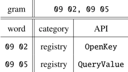
Figure 2.1: An example of a 2-gram at MIST level 1 with description of components
Figure 2.1 displays an example a 2-gram. The gram09 02refers to theregistry API
callOpenKey, and the gram09 05refers to theQueryValueAPI call which is also in the
registry category. Hence, the 2-gram 09 02, 09 05 refers to the behavior of opening a
registry key then querying a registry value. Without argument information, it is impossible to discern whether the executable is querying the value of the key that it just opened or if the query targets a different registry key.
03 05 00000001 00dc3932 00a93b39 002c392d ba92d7c6 MoveFile flags source file ext source file path dest file file dest file path
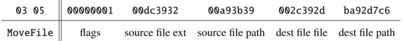
Figure 2.2: An example of a 1-gram at MIST level 2 with description of components
At MIST level 2, the grams include a level of function argument information.
Figure 2.2 shows an example of a 1-gram at MIST level 2. First, the 03 05 part refers
to the filesystem APIMoveFile. Then there is a series of hash-encoded components that
represent different parts of the argument information. MIST level 2 contains the more
generic arguments, which would be common within a family of malware, but not arguments
that are likely to be specific to a specific variant. For theMoveFileAPI, for example, the
generic arguments include
• flags that represent filesystem move options,
• the source file, which includes
the file extension and
the path in the file system (not including the file name), and • the destination file location, which also includes
the file extension and the path.
On the other hand, MIST level 2 does not include the actual file base names. Such specifics would fall into a MIST level 3. Not every API call requires the same number of arguments, so only the arguments that are present in the behavior report get encoded into MIST format.
This representation also allows effectiveness of geometric clustering techniques,
Rieck reports that a quad-core Opteron 2.4GHz system processes at a rate of 15,000 reports per day and uses 5GB of memory during regular clustering.
2.3.2 Behavior Analysis.
Rieck et al. implement hierarchical clustering with Euclidean distance complete linkage (HCL) [26]. Training starts with 3,133 samples from Sunbelt Software that come from 24 malware families that each have no more than 300 members. This labelled training set forms a reference to start the clustering process. After clustering on a set of 33,698 samples the algorithm finds 434 clusters which each contain 69 reports on average. Rieck shows high consistency of the top ten clusters with respect to Kaspersky labels, which
indicates that the clusters represent the differing families of malware by behavior. Rieck
explains that the majority of inconsistency that does occur comes from antivirus industry labels. The Rieck paper does not provide time measurements for collecting the dynamic analysis data.
Bailey et al. perform single-linkage hierarchical clustering on malware behavior [2].
They use a high-level view of behavior, recording only the non-transient changes to the
system that persist after execution completes. For example, a malware file might enumerate the file system to get all the filenames present on the system then write those filenames to a file. Such behavior would be of value to an adversarial intelligence operative. Only the output file persists as evidence of the behavior of the malware, and the transient activity of the filesystem enumeration does not factor into their analysis. Bailey claims that this method avoids obfuscation of static analysis and low-level API sequences. They use the Backtracker system in VMware with Windows XP. They collect behavior data from 3,698 malware samples from the Arbor Malware Library (AML) over six months [1].
TheO(N2) normalized compression distance step of the Bailey process takes the most
time in both time and memory space as the number of samples rises to 500, compared to the preprocessing and clustering steps. The whole process takes about 220 seconds and
only 300MB of memory for 526 samples. On a 3,698 sample set, the method finds 403 clusters. Since 311 files do not exhibit any behavior during the process, Bailey claims a 91.6% detection rate, and then compares that detection rate to a 51.5% detection rate of Symantec. The report lists the common limitations of dynamic analysis, but does not assign a root cause to any of the files that failed to behave during observation. Bailey et al. do not run the process on non-malicious files to compare how closely other executable files compare to malicious files or to measure false positive tendencies of the high-level method [2].
Bayer et al. cluster 75,000 behavior reports within three hours and four gigabytes of
memory with an Anubis system extended withtaint tracking[3, 5]. As above, taint tracking
labels the memory address to where a function returns a value, then records when another function uses that value as input or changes the value by writing into the same location again. This tracking allows a low-level emulator to gain insight into how programs interact with the operating system and produce a behavior report for the sandbox system. The blazing performance is due to the locality-sensitive hashing (LSH) clustering algorithm which approximates the distance measurements to achieve a good result quickly that is within a threshold parameter of the optimal solution.
Hu presents a malware detection system MutantX and a malware clustering system
Duet [14]. The Duet dynamic analysis component uses binary features of n-grams of
system calls from strace call traces (q-grams). This method employs the system call
name and a canonical category to inform each datum, leaving out information from call arguments, which is similar to MIST level 1 [29]. The method does not specify how many features to select. Hu performs both static and dynamic analysis on 5,647 malware samples,
and normalizes the feature vectors onto the unit circle. The static method computesn-grams
of instruction sequences from a disassembly of the executable file. Hu notes that static analysis fails on 655 samples, while dynamic analysis fails on 645 samples. However,
only with 72 samples do both methods fail. Comparing successful processing of samples using static 3- and 4-grams and dynamic 3- and 4-grams with combined behavior and static features, Hu finds 10%–15% improvement in successful processing with the combined information. This method fusion brings the clustering method to 98.72% coverage (72 samples failed of 5,647).
2.4 Summary
This thesis analyzes aspects of several other efforts. Table 2.1 summarizes similarities
and differences of this and other works. None of those studies take advantage of as
large a sample set, although Rieck is the closest with about a third as many, and none obtain samples from OpenMalware or US-CERT. Of the researchers that pursue a dynamic analysis approach, only Bailey does not capture API calls, instead noting only the persistent changes to the sandbox that remain following execution of the sample.
Two other of those efforts make classification between two or more sets a goal, while
three seek to cluster a single body of samples by measuring similarity. One who choses to cluster implements an ensemble learning method, and one that classifies implements an
ensemble (of a different sort). This study does not use ensemble methods because pilot
tests show that fast ensembles are not as accurate as decision trees and accurate ensembles are slower than decision trees.
The details of these comparative studies reside in Table 2.2, where only one other uses a MIST representation for feature generation. Indeed, that research is first to publish the MIST, and while some other papers note the MIST in citations, none publish work that implements it. Only Kolter and Maloof use nearly as long gram structures, although that research uses static grams rather than behavior-based grams. Also, using long grams means the feature space gets very large, and only this study and Kolter and Maloof employ feature selection. Three papers mention normalizing feature vectors, but only this work publishes a comparison of normalized and non-normalized results.
Most of the studies use the same sorts of machine learning techniques. The k-nearest-neighbors (kNN) algorithm is popular both for clustering and classification, and the other clustering studies use HCL. The other two classification studies make a point to compare the common algorithms of na¨ıve Bayes (NB) and SVM with the J48 decision tree in WEKA. Firdausi adds a multilayer perceptron (MLP) classifier to the model comparison, which trains in acceptable time with as few of samples in that study.
The set of studies that the summary tables cover is not exhaustive of all malware detection research, but the tables do contain the primary publications to date that bear major points in common with the research reported in this thesis.
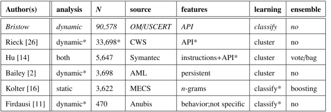
Table 2.1: Overview summary of related work. An asterisk (*) denotes similarity to this research.
Author(s) analysis N source features learning ensemble Bristow dynamic 90,578 OM/USCERT API classify no
Rieck [26] dynamic* 33,698* CWS API* cluster no
Hu [14] both 5,647 Symantec instructions+API* cluster vote/bag
Bailey [2] dynamic* 3,698 AML persistent cluster no
Kolter [16] static 3,622 MECS n-grams classify* boosting Firdausi [11] dynamic* 470 Anubis behavior;not specific classify* no
Table 2.2: Detailed summary of related work. An asterisk (*) denotes similarity to this research.
Author(s) l n M norm model result
Bristow 1,2 1-16 500 both J48 99.4% acc., 0.999 AUC
Rieck [26] 1,2* 1-4 sparse/all yes HCL 80% recall
Hu [14] 1 3,4 all yes kNN 70% covg., 0.9 prec.
Bailey [2] NA 1 all no HCL 91.6% acc.
Kolter [16] NA 1-10* 10-10,000* no kNN,NB,SVM,J48* 0.9958 AUC Firdausi [11] 1 1 116&11 no kNN,NB,SVM,J48*,MLP 96.8% acc.
III. Methodology
B
inary files execute a sequence of application programming interface (API) calls.This sequence represents the behavior of the executable file [26]. Let each API
call along with the arguments represent one action. If a program writes to a file in the
Windows operating system, the first action is to call theCreateFileAPI with arguments
that identify the file to open for writing. On success, the API call returns a valid handle to
the open file. With the handle, the program then calls theWriteFileAPI to put data into
the file. A benign word processing program uses these API calls to save a users file, but some malicious programs use these API calls to save a record of keystrokes without user knowledge.
3.1 Problem Definition
The specific sequence of API calls defines the behavior of a program. Certain
sequences occur in legitimate software, but to some extent different sequences occur in
malware. This study examines the effects of malware instruction set (MIST) feature
generation on enterprise-level malware triage. 3.1.1 Goals and Hypothesis.
The goal of this research is to determine an efficient and effective method to detect malware. The hypothesis is that certain feature selection parameter levels lead to machine
learning performing with higher accuracy and efficiency at detecting malware compared to
other levels.
This thesis addresses the following:
• Strategic Goal: Detect malware efficiently and effectively.
• Hypothesis: Certain parameter levels enable more effective malicious file identifica-tion.
3.1.2 Approach.
The approach of this effort is to compare the efficiency and effectiveness of machine learning techniques with various levels of key feature selection parameters at classifying executable files. This study employs the MIST feature generation technique to encode behavior report information into a hierarchical format [26].
The experimental levels provide the basis for comparison relative to the same input sample set. The sample set results from random sampling of the large set. Standard techniques such as antivirus or previous analysis results validate the large sample set as malicious or not.
3.2 System Boundaries
The System under Test (SUT) in this experiment is a Malware Detection System (MDS). The MDS accepts a workload of known, labeled training sample executable files or unknown executable files, and it provides a malware detection service that identifies executable files which display malicious behavior. The dynamic analysis engine
component creates dynamic analysis reports based on observed events. The feature
generation component translates the behavior reports into MIST format and generates
q-grams before selecting the most useful grams as features by filtering by information gain.
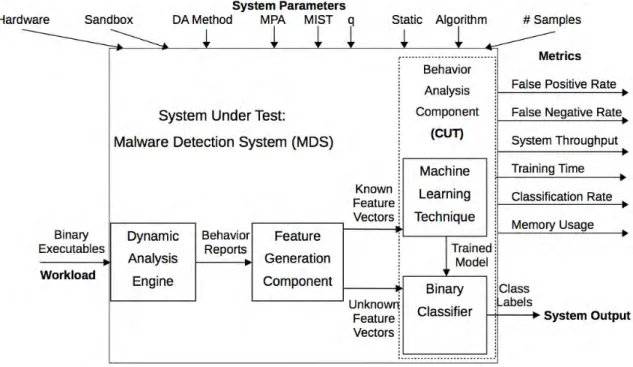
The behavior analysis component is the Component under Test (CUT), which accepts sets of feature vectors and provides malware detection and classification capability. The block diagram in Figure 3.1 depicts the SUT and its components.
While this study measures the timing of a specific dynamic analysis engine known
as Cuckoo Sandbox using VirtualBox, comparing timing measurements of different
Figure 3.1: Malware Detection System Component Diagram
does not rely on a specific dynamic analysis engine implementation since all known implementations have the potential to create behavior reports that meet the requirements of the MIST feature generation technique. Similarly, this study does not depend on a
specific computing platform. While this research effort validates this method on Microsoft
Windows XP Service Pack 3 virtual guests, the concept extends to all other common operating systems where API call observation is possible through analogous methods.
3.3 System Services
The malware detection system detects malware within a set of unknown executable files by building a model from information the system discovers in a training set of
executable files. A set of non-maliciousbenignfiles and a set of known malware samples
comprise the training sample set. The system outputs a cryptographic hash of the
The class labels derive from the labels correlated with the known training sample set. Thus,
the approach is an example ofsupervised learning.
The success outcome is when the class label is correct for an executable file. A failure outcome is when the class label is incorrect. For failures, either the label indicates that
the executable file is malicious when it is in fact benign, which is an example of a false
positive, or the label indicates a benign file that is in fact malicious, an example of afalse negative. False negatives are undesirable because they represent a missed opportunity to detect a malicious program, which means that an adversary retains the capability provided by that program. The false positive rate of a malware detection system allows operators to calculate how much wasted overhead the analysts must manually review.
The system discards samples if there is not enough behavior in a report and is therefore not desirable for input to clustering or classification algorithms. The cutoffthreshold of the number of actions required is a result of applying domain knowledge and inspecting the smallest reports to find an appropriate level. There are 4,038 out of 90,578 total samples in this study that do not perform any actions. If a malware sample does not display behavior,
then there is either some difference between the malware target environment and the test
environment, or the sample simply does not perform any behavior. The system need not learn from nor detect malware samples that do not perform any behavior. Cyber defenders must take steps to ensure that a test environment matches the target environment in the enterprise in order to ensure that malware targeted for that enterprise performs behavior in the test environment.
Another failure outcome occurs when no features from the selection list of the top features, by information gain, that come from a sample. Such samples do not contribute information to that specific level of parameter levels. Thus a drawback exists from limiting the number of features. On the other hand, there exist millions of potential features at
with hundreds of millions of dimensions. This curse of dimensionality requires attention when cyber analysts select a feature selection method for a machine learning scheme. This method deals with the large number of potential features by selecting the top 500 features according to information gain.
3.4 Workload
The workload this study provides to the SUT represents a set of executable files from an enterprise cyber infrastructure (ECI). A cryptographic hash of the contents of an executable file identifies the file in the workload. Identifying files by hash allows
the system to treat two executable files that differ by a single bit or more as separate.
Although file source data such as filename and source host are available to host analysis teams, such data are outside the scope of this experiment. A default installation of the Microsoft Windows XP Service Pack 3 operating system contains thousands of unique binary executable files, and a newly installed application may contain one to hundreds of executable files. Additionally, each update applied to an operating system or application adds or modifies one to hundreds of executable files at a time. Such updates introduce variability to a given ECI. Therefore, the distribution of input executable files to the SUT strongly depends on the individual ECI. The sample set consists of benign software samples similar to the most generic ECI. The distribution of specific software products does not necessarily affect the overall performance of a learned model because different versions of software that accomplish the same generic service likely exhibit similar behavior.
A current limitation of the Cuckoo Sandbox configuration pushes the ability to operate 64-bit guests outside the scope of this research, but the Cuckoo Sandbox developer intend to provide 64-bit capability in the future. Thus, this study uses 32-bit executable file samples in a 32-bit Windows XP SP3 guest. Cyber operators should ensure that the sample set for an operational malware detection system includes samples germane to the operational cyber infrastructure.
This study uses a set of malware from the US-CERT and Open Malware malware collections, which reflect many types of malware, including backdoors, constructors,
sniffers, droppers, spyware, viruses, worms and trojans [25, 30]. This research randomly
selects a subset of 64,987 32-bit Windows (Portable Executable format) malware samples from this large collection.
The whiteware set includes executable files from operating system vendor media, with the assumption that these executable files do not perform malicious behavior. Cyber defenders must add additional whiteware samples from installations of common types of user applications that occur in the enterprise cyber infrastructure. The white samples for this study originate from known clean Microsoft Windows media from Windows 2000 to Windows 7. This study uses a total number of 25,591 whiteware samples, and the total number of samples in the data set comes to 90,578.
The large number of malware samples from a very large collection precludes a detailed analysis of malware families within the scope of this study. However, this research uses a large number of samples randomly selected from a collection that contains a wide variety of malware. Therefore, the training set of malware executables has the potential to contain a wide variety of unique malicious behaviors. Other studies show that malware families usually perform similar behaviors, so whichever variants randomly appear in the training set contribute to the available training information for the learning algorithm. It is possible that a large malware family randomly present in the training set could introduce a bias toward detecting that family, however if such a family is more prevalent in the wild then detecting that family is a desirable trait. Operationally, cyber defenders should tailor the training set to the types of threats that face the particular enterprise.
3.5 Performance Metrics
The performance of the SUT comes from several measurements. The classification accuracy rate (%acc) of the malware detection model is the number of correctly-classified
samples divided by the total sample size (percent correct). The false positive rate (FPR) is relevant for evaluating how many files the cyber analysts must manually review. The false negative rate (FNR) indicates the importance of a defense in depth strategy including alternative detection capabilities. A receiver operating characteristic (ROC) curve of a classifier graphs the true positive rate versus the false positive rate. Comparing several ROC curves shows the relative tradeoffs in false positives and false negatives. This study uses the area under the ROC curve (AUC), which is a summary of the ROC curve for a classifier, because it is simpler to compare 64 experimental classifiers by AUC than attempting to display and view all 64 ROC curve plots. Some relative false negative and false positive information is available in a full ROC plot that is not available in the AUC summary, but the AUC is suitable for this study.
In addition, the throughput of the SUT is the number of files that the system processes per unit time. The training time is the time the system requires to build a model from a specific machine learning technique with a given training set and feature selection parameter level.
3.6 System Parameters
Many parameters impact the performance of the SUT. The specific implementation of the dynamic analysis (DA) engine, feature generation component and machine learning component each require inspection of several relevant parameters.
3.6.1 Dynamic Analysis Engine.
Increased hardware capability increases the potential to execute additional jobs in parallel. This study utilizes available hardware to run 12 sandboxes in parallel. The operating system affects certain specifics of the implementation, but not the general concept under study [9]. This research uses a Dell server with two six-core Intel Xeon 2GHz processors and 500GB system memory. The operating system is 64-bit Ubuntu 12.04
Desktop (the sandbox environment requires the desktop version rather than the server version).
Emulation or virtualization has various effects, but the investigation of the differences of such effects is outside the scope of this study [9]. This study uses full operating system virtualization with Oracle VirtualBox [22].
Various types of hooking capture API calls; Cuckoo Sandbox uses dynamic link
library (DLL) injection. The DLL injection method gets in the way of the test program calling API calls and logs all the calls before forwarding them to the operating system. Instruction-level tracing with data taint analysis captures behavior a different way, but an experimental comparison between the methods is outside the scope of this study. Any method that produces a MIST-compatible behavior report can contribute to this method.
Some publications do not report the dynamic analysis timeout, which is normally five minutes. This methodology employs a 15 second timeout in order to increase throughput.
Comparing different timeouts is outside the scope of this study. The goal is to capture any
malicious behavior during processing, but some files take a long time to execute. This study assumes that most malware completes malicious behavior quickly, within about five seconds. The timeout is higher, at 15 seconds, in order to allow sandbox initialization and the API hooking time to complete before the file executes. This assumption means that the system does not detect malware that waits 15 seconds or more to execute malicious behavior. However, even waiting for five minutes does not guarantee enough time to discover all malicious behaviors. A malware author is able to evade a detection system that has a particular timeout by finding out what the timeout is.
Multiple path analysis (MPA) might help solve the timeout problem. MPA
increases the potential to detect obfuscation and avoid long delays, but requires additional computational time according to the branching factor of the file under analysis [20]. Experimenting with multiple path analysis is outside the scope of this study.
3.6.2 Feature Generation Component.
MIST level 1 records API name and category, and level 2 adds generic argument information (if present). Level 3 adds specific argument details. This study explores both
level 1 and level 2. The parameterqis the length ofq-gram instruction sequences. Previous
studies useq=2 orq=4, and this study researches the effects of lengths from 1–16. Feature selection uses information gain as a measurement of feature usefulness. The
system keeps the top 500 features (q-grams), which is the same as the number Kolter
and Maloof use as feature selection for training decision trees. Kolter and Maloof
find 68,744,909 distinct static n-grams from a set of 476 malicious executables and 561
benign executables, and hence select the top 500 of thosen-grams [16].
However, as Section 4.1 reports, this method finds from 85–4,171 grams at MIST level 1 and from 1,499,980–17,686,084 grams at level 2 although using a larger sample set of 90,578 samples total. This method finds far fewer distinct grams because the MIST behavior report gram space is more sparse than the binary file byte gram space in the static
experiments. Since keeping 500 out of 68 million works best for the staticn-gram method
for Kolter and Maloof, then 500 should be sufficient out of 17 million features, since the
features go to the same machine learning technique (J48). In addition, each feature from this behavior-based method potentially represents more information than arbitrary bytes extracted from the binary file. Therefore, this method should not require more features
than the static n-gram method in order to represent useful information for the learning
algorithm. However, if fewer features would perform just as well as 500, then including all 500 should only hinder computational burden and not classification accuracy. Therefore investigating the effects of different feature space sizes is outside the scope of this study.
3.6.3 Machine Learning.
This study uses the Wakaito Environment for Knowledge Acquisition (WEKA) J48 implementation of the C4.5 decision tree learning algorithm [13]. This study uses 64,987
malicious and 25,591 benign executable files, for a total set of 90,578 samples. The malicious files come from a combination of malware sets from US-CERT and Open Malware [25, 30]. The benign files come from known clean Microsoft Windows operating
system install media. The experiments use 10-fold stratified cross validation in order
to measure generality. Each machine learning algorithm sees the same set of folds per repetition.
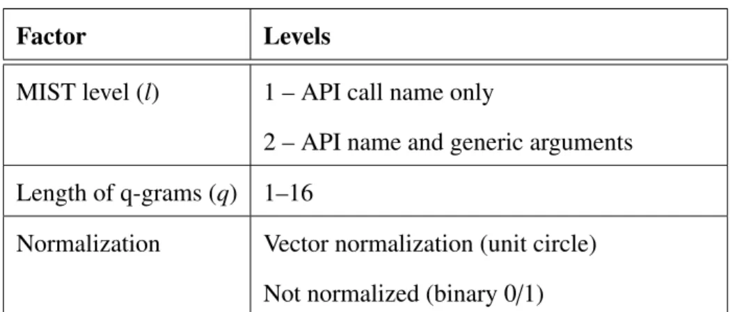
3.7 Factors
The factors for this experiment are the MIST level, the length of q-grams (q), and
whether or not the feature vectors undergo normalization. This experiment evaluates two MIST levels: the level without any argument information and the level with partial,
non-specific, argument information. The levels of q range from 1 through 16. Gram lengths
longer thanq= 16 lead to computationally prohibitive feature selection. The normalization
factor includes two levels: non-normalized, which leaves the feature vectors as vectors of ones and zeros, and normalized, which applies basic vector normalization to project the magnitude of the vector onto the unit circle while maintaining the direction. Several authors mention these factors during similar research [2, 4, 16, 26].
Table 3.1: Factor Levels
Factor Levels
MIST level (l) 1 – API call name only
2 – API name and generic arguments
Length of q-grams (q) 1–16
Normalization Vector normalization (unit circle)
3.8 Evaluation Technique
This experiment measures an instance of the CUT. Standard 10-fold cross-validation measures the generality of each model.
A number of the dynamic analysis runs undergo manual validation. This practice validates that the dynamic analysis component records malicious behavior.
3.9 Experimental Design
The methodology employs a full-factorial experimental design for a total of
2×16×2=64 experiments. Each experiment undergoes 10 repetitions to explore the
distribution variance in addition to the 10-fold cross validation, so each factor level undergoes 100 runs total. The cross validation is stratified so that class distributions remain
similar throughout the process. Furthermore, each different experiment sees the same set
of cross validation folds so that the relative mix of samples does not affect the variation
in the results. Analysis uses a 99.9% confidence level to determine statistical significance. Since the goal for false negative rates is less than 0.1%, measurements need to have enough confidence to make a significant difference.
3.10 Methodology Summary
This method of malware detection involves detailed executable file classification. To determine which of the selected factor levels performs best in this domain, each factor tests
on the same sample sets with the J48 learning algorithm. The input data areq-gram feature
vectors from MIST feature generation based on dynamic analysis reports. Any dynamic analysis engine that can translate behavior reports into MIST format can compare to the results of this study.
IV. Results and Analysis
T
his chapter reports results and detailed analysis of the dynamic analysis engine, thefeature generation component, and the machine learning component by the 6,400 experiment runs. First, Section 4.1 covers feature selection. Next, Section 4.2 presents the effects of the malware instruction set (MIST) level (l) and q-gram length (q) factors
on classifier performance. Then Section 4.2.2 contains the effect of normalization, and
Section 4.3 presents findings on the effective sample set size. Last, Section 4.6 analyzes
limitations of this research and dynamic analysis at large.
4.1 Feature Generation and Selection
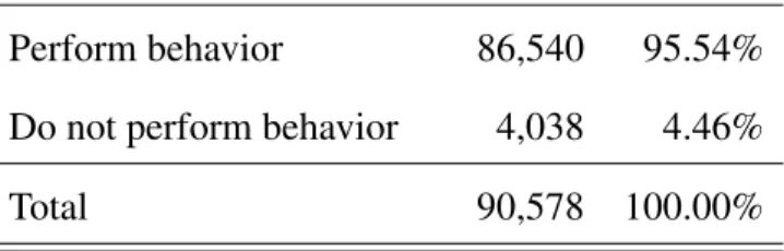
After dynamic analysis of the 90,578 samples, there are 4,038 samples that do not exhibit behavior. Table 4.1 displays the dynamic analysis results. Section 4.6 discusses reasons for those 4.46% of samples not yielding behavior. The 86,540 samples that do
perform behavior, which make the other 95.54% of the total set, exhibit 85 different
application programming interface (API) calls. That is, at MIST level 1, there are 85
unique 1-grams in the behavior reports. For example, in the 1-gram 03 04, the number
03refers to the filesystem category, and04refers to theMoveFileAPI call.
Table 4.1: Summary of dynamic analysis performance
Perform behavior 86,540 95.54%
Do not perform behavior 4,038 4.46%
Total 90,578 100.00%
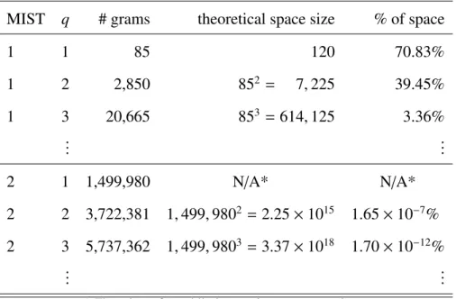
Table 4.2: Detailed examples of feature generation component results
MIST q # grams theoretical space size % of space
1 1 85 120 70.83% 1 2 2,850 852 = 7,225 39.45% 1 3 20,665 853 =614,125 3.36% ... ... 2 1 1,499,980 N/A* N/A* 2 2 3,722,381 1,499,9802 =2.25×10¹⁵ 1.65×10⁻⁷% 2 3 5,737,362 1,499,9803 =3.37×10¹⁸ 1.70×10⁻¹²% ... ...
* There is no formal limit on unique argument data.
for three examples from each MIST level. When q = 2, there are 2,850 unique 2-gram
sequences in the behavior reports, which is only 39.45% of the possible 2-long sequences
of those 85 API calls. For example, the gram09 02refers to the registry API callOpenKey,
and the gram 09 05 refers to the QueryValue API call which is also in the registry
category. Hence, the 2-gram09 02, 09 05refers to the behavior of opening a registry key
then querying a registry value. Without argument information, it is impossible to discern whether the executable is querying the value of the key that it just opened or if the query targets a different registry key.
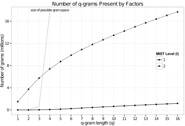
As the value ofqincreases, the number of uniqueq-grams that occur in the behavior
reports also increases, but not as fast as the number of possible grams. Each additional entry in a sequence multiplies the total possible number of permutations of grams by the number of possibilities for that entry (e.g. 85 in this data set). Hence, 3-grams have 853= 614,125
of possible grams increases exponentially with gram length, but the grams that occur in the data set do not fill up that space.
Figure 4.1: Graph of the number of millions of uniqueq-grams present in the data for each
level of the MIST level (l) and gram length (q) factors with depiction of the size of the
space of possible grams for MIST level 1
For MIST level 2, which records one level of function arguments, the number of possible gram variations is much higher. There are 1,499,980 unique 1-grams within the behavior reports of this data set at MIST level 2. This occurs because the arguments can be any value that the program could provide to that API call. Figure 4.1 indicates that, as with
MIST level 1, the number of unique q-grams does not increase exponentially, but rather
4.2 Classifier Performance
This section reports that the MIST level factor contributes the largest effect to classifier
performance and normalization does not significantly affect performance with this data set.
The level of significance for the confidence intervals is 0.001 (i.e. 99.9% confidence that the true mean falls within the interval).
4.2.1 Overview.
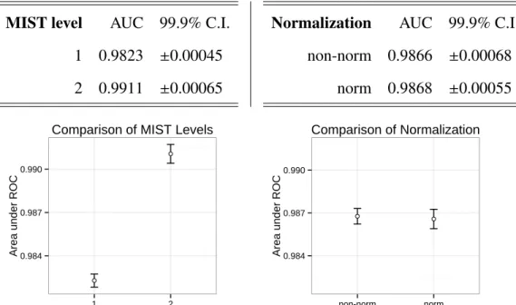
Figure 4.2 shows that MIST level 2 dominates level 1 on this data set. Over the entire data set, MIST level 2 averaged an area under the receiver operating characteristic
(ROC) curve (AUC) of 0.99106±0.00065 at the 99.9% confidence level. The additional
information that MIST level 2 includes over level 1 appears to better inform the resulting decision tree model. Additionally, 10 repetitions are clearly sufficient to characterize the majority of the variation amongst runs of the algorithm on this data set. This could mean that a lower number of repetitions would still prove sufficient in an operational environment where saving computation time improves reaction time. The following subsections provide more detailed analysis regarding the results of the experiments.
4.2.2 Normalization.
Figure 4.2 also shows that normalization does not attain a statistically significant effect on classifier accuracy at the 99.9% confidence level (nor at 95% confidence). Machine learning methods usually use normalization to reduce the bias of samples that contain a larger proportion of features because normalizing sets the magnitude of each feature vector to one without changing the direction of the vector.
Since normalization does not affect classification performance with this data set, then either the classifier is not sensitive to sample vectors that have a comparatively large magnitude, or the data set does not contain very many samples that yield large vectors. A larger feature vector is the result of a sample that performs more behaviors that the feature selection filter accepts. A data set does not fully demonstrate the normalization benefit if
MIST level AUC 99.9% C.I.
1 0.9823 ±0.00045
2 0.9911 ±0.00065
Normalization AUC 99.9% C.I.
non-norm 0.9866 ±0.00068 norm 0.9868 ±0.00055 0.984 0.987 0.990 1 2 MIST Level
Area under ROC
Comparison of MIST Levels
0.984
0.987 0.990
non-norm norm
Area under ROC
Comparison of Normalization
Figure 4.2: Details and chart of area under ROC comparisons of classifier performance by MIST level and normalization with 99.9% confidence intervals
there is a very small percentage of vectors with more attributes present compared to other vectors.
4.2.3 MIST andqDetails.
Figure 4.3 shows that MIST level 2 consistently performs at a higher AUC than MIST
level 1 except where theq-gram length reaches 15 and 16. MIST level 1 also reaches lows
atq = {15, 16}. The 99.9% confidence intervals validate that the differences between the means are significant for the rest of the levels. Some potentially outlying data points include q={7, 15, 16}for both MIST levels 1 and 2 because each of those points are greatly lower than the points around them. Further examination of those outlying results continues below in Section 4.3. Appendix B provides tables with further details on measurements from each experiment.
0.97 0.98 0.99 1.00 1 2 3 4 5 6 7 8 9 10 11 12 13 14 15 16 Gram Length (q)
Area under ROC
Key_MIST_Level
1 2
Comparison of MIST Levels and q-gram lengths
Figure 4.3: Area under ROC comparison of classifier performance by MIST level and
q-gram length with 99.9% confidence intervals
4.3 Number of Samples
Of 90,578 samples total, 86,540 samples, 95.54%, yield behavior in this dynamic methodology. Figure 4.4 shows that the number of samples steadily decreases as the levels of the factors increases, which reveals that a large percentage of samples from the dynamic
analysis results lose representation at high MIST level andq-gram length.
There are more unique q-grams both when grams are longer and when adding
argument data. Thus, the 500 features that win selection comprises a much smaller
percentage of the set of all possible features. Hence many samples no longer contain a selected behavior. This effect seems to be especially strong forq= {15, 16}.
30 50 70
1 2 3 4 5 6 7 8 9 10 11 12 13 14 15 16
Gram Length (q)
Sample Size (thousands)
Key_MIST_Level 1
2
Resulting sample sizes by MIST Levels and q-gram lengths
Figure 4.4: Comparison of resulting sample sizes by MIST level and gram length
The size of the sample set does not affect model performance as much as the amount
of information available from each sample. Figure 4.5 at first shows a slight positive correlation between sample set size and classification accuracy for MIST level 1, however there seems to be a compounding factor. The labels of the interesting points from Figure 4.3 indicate that the lowest performance coincides with the fewest available samples when q={15, 16}. Ignoring those outlying cases seems to reveal a slight positive correlation for MIST level 1, but a slight negative correlation with MIST level 2. Therefore, a low sample size adequately explains why learning performance is comparatively lower forq={15, 16}.
However, sample size does not explain the low performance atq = 7, which is especially
out of the ordinary atq= 7, even though those values do change wildly withq= {15, 16}. The same is true for classification accuracy by the percent correct measure.
l2-q16 l2-q15 l1-q16 l1-q15 l2-q7 l1-q7 0.97 0.98 0.99 1.00 30 50 70 90
Sample size (thousands)
Area under ROC
Key_MIST_Level
1 2
Performance according to resulting sample size
Figure 4.5: Performance with 99.9% confidence intervals according to sample set size after removing zero-vectors with selected labels by MIST level (l) andq-gram length (q)
The increasing levels of the MIST and q-gram factors yield feature vector sets of
decreasing sizes because the methodology discards vectors that equal zero. Such vectors do not provide useful information to a model because it represents an executable file that exhibits no behavior. However, some files that do exhibit behavior end up with a feature vector of zero because only 500 features survive feature selection. This feature size parameter agrees with the number that Kolter and Maloof find useful for learning based on static 4-grams [16]. The usefulness of this level of the parameter arises from both
the learning algorithm and the implicit dimensionality of the input data. Although this
methodology differs from Kolter and Maloof regarding the source of the input data (the
implicit dimensionality may differ), the learning algorithm is the same. That is, since 500
features works for the decision tree algorithm of Kolter and Maloof, then it is feasible that 500 features approximates a useful feature size for the decision trees in this study.
Kolter and Maloof find 68,744,909 distinct staticn-grams from a set of 1037 samples
total, and hence select the top 500 of those n-grams [16]. However, this method finds
only 17,686,084 behaviorq-grams using a sample set of 90,578 samples total. This method
finds far fewer distinct grams because the MIST behavior report gram space is more sparse than the binary file byte gram space in the static experiments. Table 4.3 shows the selection rates for the first three levels ofqfor MIST levels 1 and 2.
Table 4.3: Detailed examples of feature selection rates
MIST q # grams features % of grams
1 1 85 85 100.000% 1 2 2,850 500 17.544% 1 3 20,665 500 2.420% ... ... 2 1 1,499,980 500 0.0333% 2 2 3,722,381 500 0.0134% 2 3 5,737,362 500 0.0087% ... ...
Since keeping 500 out of 68 million works best for the staticn-gram method for Kolter
and Maloof, then 500 could be sufficient out of 17 million features, since the features go
input to machine learning in both studies. In addition, each feature from this behavior-based method potentially represents more information than arbitrary bytes extracted from the binary file. Therefore, this method represents more semantic information per feature
than the staticn-gram method.
Operationally, cyber operators should select a set of features that is large enough to represent the number of unique behaviors that benign and malicious programs perform. Then the machine learning algorithm discovers the relationship between the behaviors and the maliciousness of executable files from the training samples.
4.4 Timing Analysis
The dynamic analysis component takes 12 days to generate behavior reports from the 90,578 samples by running 12 parallel guests in Sub VirtualBox with Cuckoo Sandbox on a Dell server with two six-core Intel Xeon 2GHz processors and 500GB system memory
on Ubuntu 12.04. The analysis timeout is 15 seconds, but each sample experiences
an additional 54 seconds of overhead on average. The overhead mainly results from processing large behavior report files from executables that log a large number of API calls. Optimizing the dynamic analysis process for speed is outside the scope of this study because commercial dynamic analysis products solve this problem.
Translating a generic behavior report out of a dynamic analysis engine into the MIST format takes less than a second for small reports, and operates in time proportional to
the length of the behavior report. Extracting the q-grams out of the MIST reports takes
2.4 minutes at MIST level 1 andq=1, and it takes 6.9 hours for MIST level 2 withq= 16.
Naturally, this processing time is proportional to the number and size of grams.
Training decision tree models with the Wakaito Environment for Knowledge Acquisition (WEKA) J48 implementation of the C4.5 algorithm on the 6400 experiment runs takes 81 days worth of computational time [23]. Using 20 parallel processes on the same hardware as above takes 4 days in the WEKA experimenter [13].