Secret key establishment from common randomness represented as complex correlated random processes: Practical algorithms and theoretical limits

Dissertations

2018

Secret key establishment from common

randomness represented as complex correlated

random processes: Practical algorithms and

theoretical limits

Mohammad R. Khalili Shoja

Iowa State University

Follow this and additional works at:https://lib.dr.iastate.edu/etd Part of theComputer Engineering Commons

This Dissertation is brought to you for free and open access by the Iowa State University Capstones, Theses and Dissertations at Iowa State University Digital Repository. It has been accepted for inclusion in Graduate Theses and Dissertations by an authorized administrator of Iowa State University Digital Repository. For more information, please [email protected].

Recommended Citation

Khalili Shoja, Mohammad R., "Secret key establishment from common randomness represented as complex correlated random processes: Practical algorithms and theoretical limits" (2018).Graduate Theses and Dissertations. 16827.

by

Mohammad R Khalili Shoja

A dissertation submitted to the graduate faculty in partial fulfillment of the requirements for the degree of

DOCTOR OF PHILOSOPHY

Major: Electrical and Computer Engineering (Secure and Reliable Computing)

Program of Study Committee: George T. Amariucai, Co-major Professor

Zhengdao Wang, Co-major Professor Yong Guan

Daji Qiao Doug Jacobson Vivekananda Roy

The student author, whose presentation of the scholarship herein was approved by the program of study committee, is solely responsible for the content of this dissertation. The Graduate College will ensure this dissertation is globally accessible and will not permit alterations after a degree is

conferred.

Iowa State University Ames, Iowa

2018

DEDICATION

I dedicate this thesis to my amazing wife, Zahra for her unconditional love, sacrificial care and support during the years of my Ph.D., and to our loving parents, to whom we owe everything and whose prayers kept me going.

TABLE OF CONTENTS

Page

LIST OF TABLES . . . v

LIST OF FIGURES . . . vii

ACKNOWLEDGEMENTS . . . ix

ABSTRACT . . . x

CHAPTER 1. INTRODUCTION TO THE INFORMATION-THEORETIC CRYP-TOGRAPHY . . . 1

1.1 Introduction . . . 1

1.2 Generating Secret Key in the case of i.i.d Random Variables . . . 3

1.2.1 OSRB Framework . . . 6

1.3 Preliminary Concepts in Generating Secret Keys for non-i.i.d Cases . . . 8

1.3.1 Information Spectrum and Smooth Entropies . . . 8

1.3.2 Randomness Extractors in Privacy Amplification . . . 11

1.3.3 Simple Binary Hypothesis Testing . . . 13

CHAPTER 2. SECRET COMMON RANDOMNESS FROM ROUTING METADATA IN AD-HOC NETWORKS . . . 16

2.1 Introduction . . . 16

2.2 Dynamic Source Routing . . . 19

2.4 Proposed Algorithm . . . 25

2.4.1 Advantage Distillation . . . 25

2.4.2 Information Reconciliation . . . 28

2.4.3 Privacy Amplification . . . 30

2.5 Simulation Results . . . 39

2.5.1 Secret Length and The Secret Bit Rate . . . 39

2.5.2 The Effects of Speed and Transmission Range . . . 44

2.5.3 Increasing The Secret’s Length by Spoiling Knowledge . . . 48

CHAPTER 3. ON THE SECRET KEY CAPACITY OF SIBLING HIDDEN MARKOV MODELS . . . 50

3.1 Introduction . . . 50

3.2 Related Work . . . 53

3.3 System Model . . . 54

3.4 Generating Secret Key Problem . . . 55

3.4.1 Sibling Hidden Markov Models . . . 56

3.5 The Secret Key Establishment Potential of the Sibling Hidden Markov Model 57 3.5.1 Upper Bound . . . 57

3.5.2 Lower Bound . . . 58

3.6 Calculating the Bounds . . . 61

3.7 Simulation Results . . . 69

3.8 Conclusion . . . 76

BIBLIOGRAPHY . . . 78

APPENDIX A. INFORMATION THEORY . . . 86

LIST OF TABLES

Page

Table 2.1 Different groups and types when we send RID in clear . . . 30

Table 2.2 Number of subsets, obtained by the na¨ıve algorithm with 1 = .001,

for RIDs sent in the clear. Total network-wide achievable number of

shared secret bits, in last column. . . 36

Table 2.3 Number of subsets, obtained by the na¨ıve algorithm with 1 = .001,

for protected RIDs. Total network-wide achievable number of shared

secret bits, in last column. . . 36

Table 2.4 Simulation Parameters . . . 39

Table 2.5 Probability Distribution of an Unknown Full Route, from Eve’s

Per-spective based on Sending RID Type . . . 41

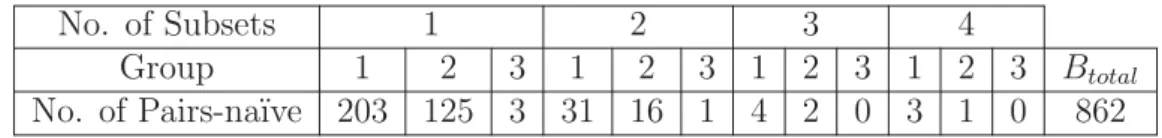
Table 2.6 Number of subsets, obtained by the na¨ıve and heuristic algorithms

with 1 = .001, when considering all full routes of length at least 3

and in the case of protected RID. . . 43

Table 2.7 Size of min-entropy based on 3 different speeds in the case of clear

RID. Speed 1, speed 2 and speed 3 are uniform (.5,1), uniform (1,1.5)

Table 2.8 Number of node pairs vs. number of subsets for three different speeds

by applying na¨ıve algorithm with 1= .001, when RID is sent in the

clear. Total network-wide achievable number of shared secret bits, in last column. Speed 1, speed 2 and speed 3 are uniform (.5,1), uniform

(1,1.5) and uniform (1.5,2), respectively. . . 45

Table 2.9 Number of node pairs vs. number of subsets for three different speeds

by applying na¨ıve algorithm with 1 = .001, when RID is protected.

Total network-wide number of shared secret bits, in last column.Speed 1, speed 2 and speed 3 are uniform (.5,1), uniform (1,1.5) and uniform

(1.5,2), respectively. . . 46

Table 2.10 Size of min-entropy based on 4 different ranges in the case of clear RID. 46

Table 2.11 Number of subsets, obtained by the na¨ıve algorithm with 1 = .001,

in the case of sending RID in clear for different transmission range. Total network-wide achievable number of shared secret bits, in last

column. . . 47

Table 2.12 Number of node pairs vs. number of subsets for five different ranges

by applying na¨ıve algorithm. Total network-wide number of shared

secret bits, in last column. . . 47

Table 2.13 Number of subsets, obtained by the na¨ıve and heuristic algorithms,

when considering only full routes of length at least 4. Total

LIST OF FIGURES

Page

Figure 1.1 Shannon’s Model to Study the Secrecy . . . 2

Figure 1.2 Wiretap Model . . . 3

Figure 1.3 Discrete Memoryless Channel Model . . . 5

Figure 1.4 Source Secret Key Generation Model . . . 6

Figure 1.5 The Model for Generating Secret Key . . . 8

Figure 1.6 Converting random variableX to a uniform random variable . . . . 10

Figure 1.7 Hmin and Hmax for random variable X . . . 12

Figure 1.8 limsup and liminf in probability . . . 12

Figure 2.1 Communication among node 1 and 5 . . . 20

Figure 2.2 The area covered by l nodes . . . 24

Figure 2.3 Example for proposed algorithm . . . 27

Figure 2.4 Number Of Full Routes vs. Full Route Length . . . 40

Figure 2.5 Number Of Pairs vs. Number of Rows in their shared Selection matrix 40 Figure 2.6 Number Of subsets of a given size (number of rows), vs. Subset size, for the na¨ıve algorithm (Clear RID) – network-wide results. . . 42

Figure 2.7 Number Of subsets of a given size (number of rows), vs. Subset size, for the na¨ıve algorithm (Protected RID) – network-wide results. . . 43

Figure 3.1 Sibling Hidden Markov Model for generating the secret key . . . 52

Figure 3.3 Dependency Graph of the Product of Random Matrix . . . 65

Figure 3.4 The upper bound secret key capacity by fixing Alice and Bob’s

emis-sion matrices and changing Eve’s crossover probability . . . 73

Figure 3.5 The lower bound secret key capacity by fixing Alice and Bob’s

emis-sion matrices and changing Eve’s crossover probability . . . 74

Figure 3.6 Comparing the lower and upper bound for four different values of

Eve’s crossover probability when Alice and Bob’s emission matrices

are fixed. CP in figures stands for crossover probability . . . 74

Figure 3.7 The upper bound secret key capacity by fixing Alice and Eve’s

emis-sion matrices and changing Bob’s crossover probability . . . 75

Figure 3.8 The lower bound secret key capacity by fixing Alice and Eve’s

ACKNOWLEDGEMENTS

This thesis was completed under supervision of my Ph.D. advisors, Professors George Traian Amariucai and Zhengdao Wang. I would like to thank Professor Amariucai for his guidance and support throughout my Ph.D. studies. His insight and advice have always guided me in my personal and professional life. I am also thankful to Professor Zhengdao Wang for his insightful discussions. I would also like to thank my Ph.D. committee members, Professors Doug Jacobson, Daji Qiao, Yong Guan, and Vivekananda Roy for their helpful suggestions.

I would like to thank my friends and labmates at Iowa State University for making my stay in Ames, Iowa memorable.

ABSTRACT

Establishing secret common randomness between two or multiple devices in a network resides at the root of communication security. In its most frequent form of key establish-ment, the problem is traditionally decomposed into a randomness generation stage (ran-domness purity is subject to employing often costly true random number generators) and an information-exchange agreement stage, which relies either on public-key infrastructure or on symmetric encryption (key wrapping).

This dissertation has been divided into two main parts. In the first part, an algorithm called KERMAN is proposed to establish secret-common-randomness for ad-hoc networks, which works by harvesting randomness directly from the network routing metadata, thus achieving both pure randomness generation and (implicitly) secret-key agreement. This al-gorithm relies on the route discovery phase of an ad-hoc network employing the Dynamic Source Routing protocol, is lightweight, and requires relatively little communication over-head. The algorithm is evaluated for various network parameters, and different levels of complexity, in OPNET network simulator. The results show that, in just ten minutes, thou-sands of secret random bits can be generated network-wide, between different pairs in a network of fifty users.

The proposed algorithm described in this first part of this research study has inspired study of the problem of generating a secret key based on a more practical model to be explored in the second part of this dissertation. Indeed, secret key establishment from com-mon randomness has been traditionally investigated under certain limiting assumptions, of which the most ubiquitous appears to be that the information available to all parties comes

in the form of independent and identically distributed (i.i.d.) samples of some correlated random variables. Unfortunately, models employing the i.i.d assumption are often not accu-rate representations of real scenarios. A more capable model would represent the available information as correlated hidden Markov models (HMMs), based on the same underlying Markov chain. Such a model accurately reflects the scenario where all parties have access to imperfect observations of the same source random process, exhibiting a certain time de-pendency. In the second part of the dissertation , a computationally-efficient asymptotic bounds for the secret key capacity of the correlated-HMM scenario has been derived. The main obstacle, not only for this model, but also for other non-i.i.d cases, is the computational complexity. This problem has been addressed by converting the initial bound to a product of Markov random matrices, and using recent results regarding its convergence to a Lyapunov exponent.

CHAPTER 1.

INTRODUCTION TO THE

INFORMATION-THEORETIC CRYPTOGRAPHY

1.1

Introduction

Information-theoretic methods are among the most important approaches in the field of security whose merit is that they require no assumptions about computational capabilities of adversaries. The introduction of these methods goes backs to 1949, when Shannon initially

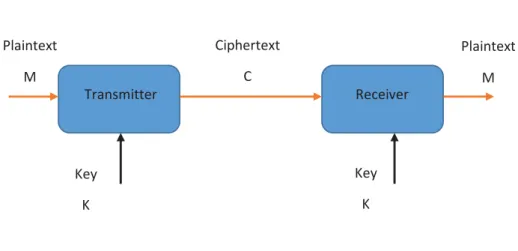
studied the secrecy based on the model in Figure 1.1.

In this model, plain text message (M) is encrypted into ciphertext (C) by applying a

shared key (K) at the transmitter, with the decryption process accomplished using the same

key at the receiver. The main goal is to transmit M in secrecy. Shannon defined the system

to be perfectly secure if knowledge of the plaintext message cannot be achieved just by

knowing the ciphertext 1.

I(M;C) = 0 (1.1)

Moreover, the receiver must have capability for decrypting the plaintext by knowing both the ciphertext and the key.

H(M|C, K) = 0 (1.2)

By considering such conditions, Shannon [1], using a combinatorial proof, showed that

H(K) ≥ H(M). In other words, the length of the key should be larger than the length

Transmitter Receiver Plaintext M Ciphertext C Plaintext M Key K Key K

Figure 1.1 Shannon’s Model to Study the Secrecy

of the plaintext, a proposition known as ”Shannon’s pessimistic result”. Yeung [2] used a

technique based on an information diagram to prove the same result.

Wyner [3] in 1975 introduced a wiretap channel and studied this models secrecy capacity.

Wyner’s model consists of two channels; the first channel is located between legitimate users (main channel) and second channel is located between a sender and an attacker (attacker’s channel). Wyner assumed the main channel to be better than the attacker’s channel and also assumed that the attacker is a passive attacker and cannot send any message into the

channels. The main goal in the wiretap model is to transmit messageM in such a way that

the attacker can obtain no information about it. Wyner showed that in the wiretap model there is no need for a pre-existing shared secret key between legitimate sender and receiver.

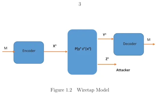
Csisz´ar and K¨orner [4] generalized Wyner’s model by assuming that the attacker’s channel is

not inferior to the main channel, and studied the secrecy capacity of the new model, depicted in Figure 1.2.

An important problem in the field of security is generating a secret key, the basic tenet of cryptography and secure communication. Generating a secret key based on information

Encoder Decoder M M Xn Yn Zn P(yn _zn_|xn₎ Attacker

Figure 1.2 Wiretap Model

In this chapter, the problem of generating a secret key between two users for the case of independent and identically distributed (i.i.d) random variables is defined, followed by the exploration of prevalent concepts and tools employed in information-theoretic methods.

1.2

Generating Secret Key in the case of i.i.d Random Variables

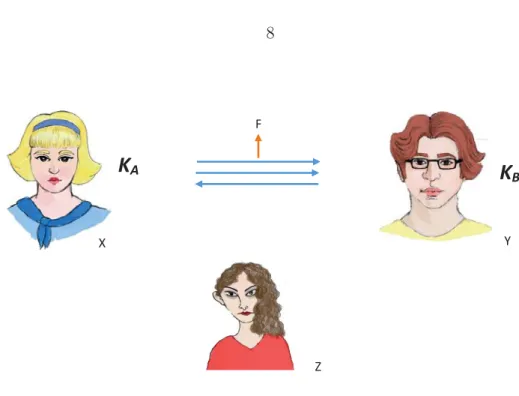
Assume i.i.d repetition of (X, Y, Z) with joint probability distribution PXY Z. In the

process of generating a secret key, Alice, who can observe Xn, wants to produce secret

common randomness with Bob, who has access toYn_{, by exchanging messageF over a public}

channel. This key should be hidden from the perspective of Eve who has side information

Zn _{and can also overhear the public communication.}

The process of generating a secret key is composed of two phases: information reconcilia-tion and privacy amplificareconcilia-tion. The aim of the former is to generate (with high probability) the same common information between the two parties. Since, in the information reconcili-ation phase, two parties using public communicreconcili-ation reveal some informreconcili-ation to a potential eavesdropper, the goal of privacy amplification is to boost the security of the generated key by extracting a (shorter) secret that is uniformly distributed over its space, given the

and KB for the secret key (Figure 1.5). This model for generating secret key is called the

source-type model. The two random variables must with high probability be the same and,

given Eve’s knowledge (F and Zn_{), their probability distribution must be uniform.}

The techniques employed in i.i.d models are based on important theorems, most related to typical sequences, packing lemma, Slepian-Wolf theorem, etc. (we have provided an

introduction to these concepts in Appendix A). In this section we will review methods for

generating a secret key in i.i.d models.

For simplicity, assume that, while Eve has no side information (there is no anyZ), she can

overhear the public communication between Alice and Bob (F). At the end of the process

of generating a secret key, KA and KB should with high probability be the same and their

distribution must be uniform. The key should also be independent of public communication. In some literature, this condition is stated as follows.

I(F;K)≤ (1.3)

We will present an accurate definition of secret key in Chapter 3of this thesis.

It can be proved that converse bound of the secret key length per observation in the i.i.d framework is RK < I(X;Y).

The achievability proof for this problem has been traditionally solved using random binning and the Slepian-Wolf theorem. Intuitively, based on Slepian-Wolf theorem, if Alice

sends nH(X|Y) bits to Bob, Bob can reconstruct Xn _{(this phase is called information}

reconciliation phase) so that both Alice and Bob have nH(X) bits at their disposal while

nH(X|Y) of these bits have been released. The secret key length per observation would

therefore be

1

PY|X Encoder Decoder M F F Xn _Yn M’

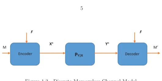
Figure 1.3 Discrete Memoryless Channel Model

As mentioned above, the exact proof of achievability is traditionally based on random

binning. Yassaee, et. al, [7] have proposed a new approach for the proof of achievability. This

proposed method, called output statistics of random binning (OSRB), can be considered as a general framework for obtaining achievability results in network information theory problems. In other words, it can be employed as an alternative approach instead of using traditional packing and covering lemmas. The main idea in OSRB is exploiting duality between problems. For example, they show that by observing the duality existing between channel coding and secret key generation, the secret-key achievability rate can be derived.

Consider a DMC with messageM and shared codebookF that can be considered as shared

randomness. By considering the model depicted in Figure 1.3 as a Bayesian network, the

joint probability distribution of this model can be written as follows.

P_MuniPFPXn|M FPYn|XnPMˆ|F Yn = (1.5)

PXnM FPYn|XnPMˆ|F Yn =

PXnPM F|XnPYn|XnPMˆ|F Yn =

PXnYnPM F|XnPYn|XnP_Mˆ_{|F Y}n

The last expression states the joint probability distribution for the generating secret key

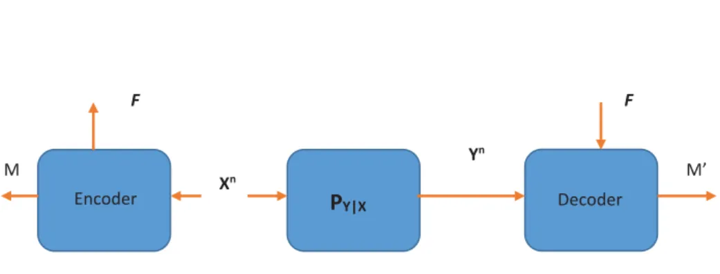
PY|X Encoder Decoder M F F Xn Yn M’

Figure 1.4 Source Secret Key Generation Model

these two models are the same and F and M are independent of one another, meeting all

the required conditions for generating a secret key.

1.2.1 OSRB Framework

As discussed earlier, the OSRB framework can be considered as an alternative method for packing and covering lemmas, and in this section, after reviewing a simple form of two important theorems in OSRB, we will employ them for solving the two earlier-mentioned important problems.

Theorem 1. Consider (Xn

1, X2n, Yn) as an i.i.d repetition of distributed sources with joint

probability distributionPX₁nX₂nYn. Then, by assuming random binning (B1 andB2) as follows:

Bi :Xin →[1 : 2nRi], i= 1,2 (1.6)

if

R1 ≥H(X1|X2Y) (1.7)

R2 ≥H(X2|X1Y)

then

E_B1B2(P˙(xn1, x2n, yn,xˆn1,xˆn2)−P(xn1, xn2, yn)1[xn1 = ˆxn1, xn2 = ˆxn2])→0 (1.8)

as n goes to ∞.

Note that ˙P is the random probability distribution induced by two random binnings.

Theorem 1is an equivalent form of the Slepian-Wolf theorem. [7]

Theorem 2. Consider (Xn

1, X2n, X3n) as an i.i.d repetition of distributed sources with joint

probability distributionPX1X2X3. Then, by assuming random binning (B1 and B2) as follows:

Bi :Xin →[1 : 2 nRi_{], i= 1,2 (1.9)} and if R1 ≤H(X1|X3) (1.10) R2 ≤H(X2|X3) R1+R2 ≤H(X1X2|X3) then E_B1B2(P˙(b1(xn1), b2(xn2), x3n,xˆn1,xˆn2)−P(xn3)Puni(b1(x1n))Puni(b2(xn2)))→ 0 (1.11) as n goes to ∞.

In this theorem bi is the realization of Bi.

To apply the OSRB framework to solving the earlier-mentioned problem of generating a

secret key mentioned, let us assume in theorem 1that if there is no Xn

2 and X1n =Xn, the

X

X Y

Z F

K

K

Figure 1.5 The Model for Generating Secret Key

result is the equivalent of the Slepian-Wolf theorem. If Alice and Bob then apply another random binning with rateRk on theXnand ifRf+RK < H(X), the output of this process is

uniformly distributed and independent of the output of the first random binning. To achieve

this result we have used theorem 2assuming X1 =X2 =X and no X3.

1.3

Preliminary Concepts in Generating Secret Keys for

non-i.i.d Cases

As mentioned earlier, the results of generating a secret key in the i.i.d cases are proved using typicality arguments, and therefore cannot be employed in non-i.i.d models. In this part the main tools to study non-i.i.d models have been explored.

1.3.1 Information Spectrum and Smooth Entropies

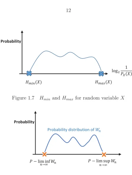
Let X be defined as a general random variable with probability distribution of PX. The

information spectrum of the random variableX is the probability distribution of the random

variable log_P1

points of the information spectrum are of importance in this regard: Hmax(PX) = max log_P1_X,

and Hmin(PX) = min log_P1_X (see Figure 1.7). Loosely speaking, Hmax(PX) is related to

the number of bits required to reconstruct the random variable X. As an example, if the

minimum probability of a discrete random variable is ₁₆1, in the worst-case scenario, X will

have 16 realizations each with probability ₁₆1. So, the random variable can be defined with 4

bits. In the same vein,Hmax(PXY|PY) is the number of required bits to reconstructX while

having perfect information of Y.

On the other hand,Hmin(PX) is roughly related to the number of intrinsic secure bits that

can be extracted from random variable X. As discussed in Definition 7and 8, a secret key

has to have a uniform distribution. So for example, when a random variableX is distributed

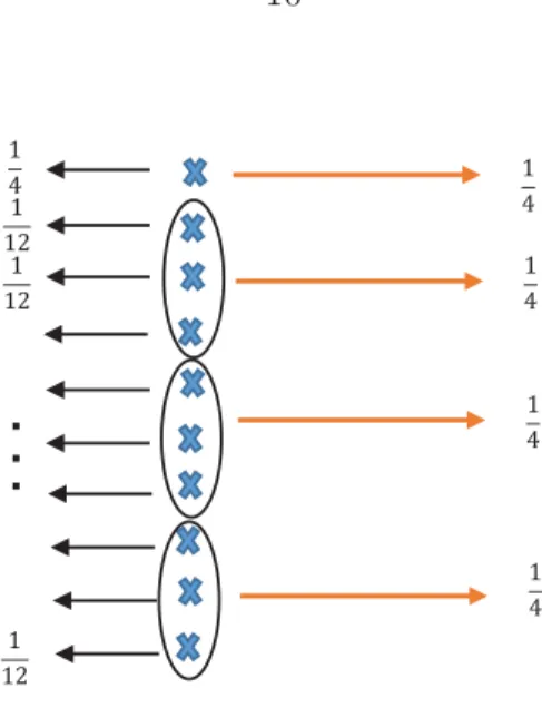
uniformly over its four realizations, two secure bits can be extracted. Let X be distributed

over ten realizations. Except one realization with probability 1₄, the probability of the rest

for each realization is ₁₂1. AlthoughX is not uniform, a uniform random variable can easily

be produced from X by bundling some realizations ofX, as depicted in Figure 1.6– in this

case, each mass point of the probability distribution of the new variable equals the maximum

of p(X). Even when bundling cannot produce a completely uniform random variable, the

result of bundling, over multiple samples, can be made close to the uniform distribution. This

closeness is usually measured by the statistical distance and will be discussed more in 1.3.2.

As intuition suggests, a form of Hmax(PXY|PY) is a fundamental term in the information

reconciliation phase where Bob (with access to Y) needs to reconstruct Alice’s signal (X).

Also, we will show thatHmin(PXZ|PZ) appears in the privacy amplification phase where Alice

and Bob need to extract random bits form X while Eve has side information represented by

(Z).

More random bits can be generated in the privacy amplification phase, and fewer bits can be sent in the reconciliation phase, if a small amount of error can be tolerated. This leads to considering probability distributions that are not identical, but statistically close to

ͳ Ͷ ͳ ͳʹ ͳ ͳʹ ͳ ͳʹ

.

.

.

Figure 1.6 Converting random variableX to a uniform random variable

the true distribution. This is the core idea of smooth entropies [8], [9], [10]. As an example,

by ignoring the smallest probabilities of a random variable, the new Hmax can move slightly

to the left of the initial Hmax of the true distribution depicted in Figure 1.7. The new

Hmax is called the smooth maximum entropy. Formally, conditional maximum entropy and

conditional smooth maximum entropy are defined as follows. Definition 1.

Hmax(PXY|PY) =−log min x∈Xy∈Y PXY PY (1.12) H_max (PXY|PY) = min QXY∈B(PXY) Hmax(QXY|QY) (1.13) whereB_(P

XZ)is the set of all non negative functions overX × Y such thatQXY ≤PXY

and d(QXY, PXY)≤, where d is the statistical distance.

Similarly, smooth minimum entropy is defined by cutting down the largest probabilities

of a random variable [8]. With this process the new Hmin will be placed on the right side

smooth minimum entropy, at the penalty that, with some small probability, the randomness extraction process will completely fail. The formal definitions for minimum entropy and conditional smooth minimum entropy are as follws.

Definition 2.

Hmin(PXZ|PZ) =−log max x∈Xz∈Z PXZ PZ (1.14) H_min (PXZ|PZ) = max QXZ∈B(PXZ) Hmin(QXZ|QZ) (1.15)

Not only are information spectrum methods useful in the single-shot scenario, but we can extend the techniques to a sequence of length n. To study asymptotic behavior of a general

sequence Wn, two fundamental probabilistic operations, i.e, limit superior and limit inferior

(Figure1.8) are defined:

P −lim sup n→∞ Wn ≡inf{α| lim n→∞P r{Wn > α}= 0} (1.16) P −lim inf n→∞ Wn ≡sup{β|nlim→∞P r{Wn < β}= 0} (1.17)

1.3.2 Randomness Extractors in Privacy Amplification

Randomness extractors are used in the privacy amplification phase. They take as input the common sequence shared between Alice and Bob at the end of the information recon-ciliation phase, and output a uniformly random (from the eavesdropper’s perspective) and usually shorter sequence to be used as a secret key. There are two types of extractors: de-terministic and seeded. In the former type, a fixed function is employed to extract secret bits from the known random variable. It can be observed that it is not possible to have a

Probability Ž‘‰ଶ ͳ ܲ_௑ሺܺሻ ܪ_௠௜௡ሺܺሻ ܪ௠௔௫ሺܺሻ

Figure 1.7 Hmin and Hmax for random variable X

Probability ܲ െ Ž‹•—’ ௡՜ஶ ܹ_௡ ܲ െ Ž‹‹ˆ ௡՜ஶ ܹ௡ Probability distribution of ܹ_௡

Figure 1.8 limsup and liminf in probability

Lemma 1. For any deterministic extractor E : {0,1}n _{→ {0,1}, there exists a random}

variable X with Hmin(X)≥n−1such that E(X)is constant.

To overcome this problem, seeded extractors are used instead. A little extra randomness

calledseed is employed in this type of extractor.

Definition 3. Strong seeded extractor

A function E: {0,1}n_{× {0,1}}d _{→ {0,1}}u _{is a (k, )-strong seeded extractor if for every}

random variable X defined on {0,1}n _{with H}

min(PXZ|PZ) ≥ k and seed random variable

R which is uniformly distributed over {0,1}d_{, the statistical distance between P}

Pu

unifPRZ is less than , where Punifu is the uniform probability distribution over {0,1}u and

Z represents the eavesdropper’s side information.

It was shown in [12] that such a function E can be constructed by two-universal hash

functions.

Definition 4. Two-universal hash functions [13]

A family of functionsF ={f :X → {0,1}u} is two-universal if

∀x=x Pf∈F[f(x) =f(x)] ≤2−u, (1.18)

where the probability is with respect to the uniformly random choice of f from the family F.

The leftover hash lemma establishes a connection between strong seeded extractors and hash functions.

Lemma 2. Leftover hash lemma [13]:

There exists a function chosen uniformly by seedRfrom two-universal familyF which can be considered as a(k,1₂2u−2k_{)-strong seeded extractor for random variableX withHmin(PXZ}|_PZ)≥

k.

The left over hash lemma directly results in

d(PfR(X)RZ, Punifu PZPR)≤

1 2

√

2u−Hmin(PXZ|PZ) _(1.19)

As intuition suggests and as discussed earlier, the minimum entropy plays an important role in the privacy amplification phase.

1.3.3 Simple Binary Hypothesis Testing

The goal of a binary hypothesis test is to map an observation into either H0 (null

decision is made to reject the null hypothesis. If the distribution of a vector variable is of interest, the following binary hypothesis test can be defined;

H0 : X ∼Pθ, θ∈Θ0

H1 : X ∼Pθ, θ∈Θ1 (1.20)

If the distribution is defined completely with the hypothesis, (Θ0 = {θ0}Θ1 = {θ1}), it

is called simple, otherwise it is composite. So, in the simple binary hypothesis test Pθ0 is

the distribution of X under the null hypothesis and Pθ1 is the distribution of X under the

alternative hypothesis. A test function Φ(x) ∈ {0,1} can be defined such that if its value

is 0, the null hypothesis has been decided which means x∈ Cc_{, otherwise, if Φ(x) = 1, the}

alternative hypothesis has been accepted, x∈ C.

Two types of error can be explored in a hypothesis test: type-I and type-II. Type-I error

(or false alarm) occurs whenH0 is true but the test choosesH1. So, in the simple hypothesis

test

PF A=Pθ0(Φ(X) = 1) =

x

Pθ0Φ(x) =EP_θ0[Φ(X)] (1.21)

Type-II error (or missed detection) happens when H1 is true but H0 is decided by the test.

So, in the simple hypothesis test

PM D = Pθ1(Φ(X) = 0) =

x

Pθ1(1−Φ(x)) (1.22)

= EPθ1[1−Φ(X)]

Although finding a region C with PF A = 0 and PM D = 0 is desirable, such a region

does not exist unless Pθ0 is singular with respect to Pθ1. In other words, by reducing the

probability of missed detection in a simple hypothesis test, the probability of false alarm

would increase. Hence, with a fixed tolerable amount of probability of false alarm, , a test

powerful test of size and the infimum of the probability of missed detection is denoted by

β(Pθ0, Pθ1). The Neyman Pearson lemma shows that such a test exists and it is given by

the following rejection region

C ={x|Φ(x) = 1}={x|L(θ0)

L(θ1) ≤K} (1.23)

CHAPTER 2.

SECRET COMMON RANDOMNESS FROM

ROUTING METADATA IN AD-HOC NETWORKS

2.1

Introduction

Automatic key establishment between two devices in a network is generally performed

either by public-key-based algorithms (like Diffie-Hellman [14]), or by encrypting the

newly-generated key with a special key-wrapping key [15]. However, in addition to the

well-established, well-investigated keying information exchange, one additional aspect of key es-tablishment is often understated: to ensure the security of the application it serves, the newly generated secret key has to be truly random. While minimum standards for software-based

randomness quality are generally being enforced [16], many applications rely on often costly

hardware-based true random generators [17]. Sources of randomness employed by true

ran-dom number generators vary from wireless receivers and simple resistors to ring oscillators and SRAM memory.

In this chapter, we build upon the observation that a readily-available source of ran-domness is usually neglected: the network dynamics. Indeed, by their very nature, com-munication networks are highly dynamic and largely unpredictable. Their randomness is usually evident in easily-accessible networking metadata such as traffic loads, packet delays or dropped-packet rates. However, as the main focus of our work is on mobile ad-hoc net-works (MANETs), the source of randomness we shall discuss here is one that is specific to infrastructure-less networks: the routing information itself. Another interesting feature of the routing information, in addition to its randomness, is that it can easily be made available to the devices that took part in the routing process, but it is usually unavailable to those

devices that were not part of the route. This idea opens the door to a whole new class of applications: with the proper routing protocol, the routing information could be used for

es-tablishingsecret common randomness between any two devices in a mobile ad-hoc network.

This common randomness could then be further processed into true common randomness, and used as secret keys.

Common randomness was pioneered in [5, 6, 18], where it is shown that if two parties,

Alice and Bob, have access to two correlated random variables (RVs) X and Y

respec-tively, (in either the source or the channel models), a secret key can be established between them through public discussions and random-binning-like (e.g. hashing) operations. The key should remain secret from an adversary eavesdropper (Eve) who overhears the public

discussions, and possesses side information (in the form of a third RV Z) correlated with

that available at Alice and Bob. Common-randomness-based key establishment generally

consists of three phases. First, Alice and Bob have to agree on two other RVs X and Y,

such thatH(X|Y)< H(X|Z) andH(Y|X)< H(Y|Z), whereH(·) is the standard Shannon

entropy. This part is sometimes calledadvantage distillation. Next, Alice and Bob (and also

Eve) sample their respective random variables a large number of times, producing sequences of values. Then Alice and Bob exchange further messages (over a public channel) to agree

on the same single sequence of values – this phase is the information reconciliation. Finally,

because the agreed-upon sequence is not completely unknown to Eve (Eve can sample her

variableZsynchronously with Alice and Bob), Alice and Bob run a randomness extractor on

it, to produce a secret key (a shorter sequence) which, from Eve’s perspective, is uniformly

distributed over its space – this is the privacy amplification phase. The ideas of [5, 6] have

been recently applied to secret key generation in wireless systems, where secure common

randomness is attained by exploiting reciprocal properties of wireless channels or other aux-iliary random sources in the physical layer [19,20,21,22,23,24,25,26,27]. One noteworthy

in practice Alice and Bob do not usually have access to large numbers of values drawn from

their random variables, but rather to only one or a few values. To address this issue, [9]

shows that for such single-shot scenarios, the smooth minimum entropy provides tight upper and lower bounds on the achievable size of the secret key.

In MANETs, the lack of infrastructure, the nodes’ mobility and the fact that packets are routed by nodes, instead of fixed devices, have resulted in the need for specialized routing protocols, like the ad-hoc on-demand distance vector AODV routing, or the dynamic source

routing (DSR) [28]. For our secret-common-randomness-extraction purposes, DSR appears

to be a good candidate, and will be the object of this work. Indeed, for generating secret common randomness between two separated nodes in the network, they must have some shared and extractable information. Among other routing protocols in ad hoc networks, DSR has this primary feature. Namely, DSR contains two main mechanisms – Route Discovery and Route Maintenance – which work together to establish and maintain routes from senders

to receivers. The protocol works with the use of explicit source routing, which means that

the ordered list of nodes through which a packet will pass is included in the packet header. It is sets of these routing lists that we shall show how to process into secret keys shared between pairs of nodes.

Our contributions can be summarized as follows:

1. We show that the randomness inherent in an ad-hoc network can be harvested and used for establishing secret keys between pairs of nodes that participate in the routing process.

2. We provide a very practical algorithm for establishing such secret common randomness, based on the DSR protocol, and we calculate a lower bound and an upper bound on the achievable number of shared secret bits, using an adversary’s beliefs.

3. We simulate a realistic ad-hoc network in OPNET Modeler, and show that within only ten minutes, thousands of secret bits can be shared between different node pairs. The rest of this chapter is organized as follows. Those parts of the DSR protocol that

are essential for understanding our algorithm are examined in Section2.2. In Section2.3, we

describe the system model and state our assumptions. Section2.4describes our proposed key

establishment algorithm. Simulation results obtained with OPNET Modeler are presented

and discussed in Section 3.7.

2.2

Dynamic Source Routing

Dynamic source routing (DSR) [28] is one of the well-established routing algorithms for

ad-hoc networks. Under this protocol, when a user (the sender) decides to send a data packet

to a destination, the sender must insert thesource route in a special position of the packet’s

header, called theDSR source route option. The source route is an ordered list of nodes that

will help relay the packet from its source to its destination. The sender transmits the packet

to the first node in the source route. If a node receives a packet for which it is not the final

destination, the node will transmit the packet to the next hop indicated by thesource route,

and this process will continue until the packet reaches its destination.

To obtain a suitable source route toward the destination, a sender first searches its own

route cache. Theroute cache is updated every time a node learns a new valid path through the network (whether or not the node is the source or the destination for that path). If

no route is found after searching the route cache, the sender initiates the route discovery

protocol. During the route discovery, the source and destination become the initiator and

target, respectively.

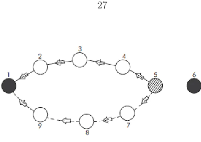
As a concrete example, suppose node 1 in Figure 2.1 wants to send packets to node 5.

Figure 2.1 Communication among node 1 and 5

discovery by transmitting a single special local broadcast packet called route request. The

route request option is inserted in the packet’s header, following the IP header. To send the route request, the source address of the IP header must be set to the address of the initiator (node 1), while the destination address of IP header must be set to the IP limited broadcast address. These fields must not be changed by the intermediate nodes processing the route request. A node initiating a new route request generates a new identification value for the route request, and places it in the ID field of the route request header. The route request header also contains the address of the initiator and that of the target. The route request ID is meant to differentiate between different requests with the same initiator and target – it should be noted here that the same request may reach an intermediate or destination node twice, over different paths. Each route request header also contains a record listing the address of each intermediate node through which this particular copy of the route request has been forwarded. In our example, the route record initially lists only the address of the initiator node 1. As the packet reaches node 2, this node inserts its own address in the packet’s route record, and broadcasts it further, and so on, until the packet reaches the target node 5, at which point its route record contains a valid route (1-2-3-4-5) for transmitting data from node 1 to node 5.

As a general rule, recent route requests received at a node should be recorded in the

node’s route request table – the sufficient information for identifying each request is the

tuple (initiator address, target address, route request ID). When a node receives a route

reply packet to the initiator, and saves a copy of the route (extracted from the route request

route record) in a table called the route cache. Second, if the node has recently seen another

route request message from this same initiator, carrying the same id and target address, or if the node’s own address already exists in the route record section of the route request packet (the same request reached the node a second time), this node discards the route request. Third, if the request is new, but the node is not the target, the node inserts its address in the packet’s route record, and broadcasts the modified packet. Fourth, if a route exists to the target address in the node’s route cache, the node sends the route reply.

In our example in Figure 2.1, node 5 constructs a route reply packet and transmits it

to the initiator of the route request (node 1). The source address in the IP header of the route reply packet is set to the IP address of the sender of the route reply (node 5). In our example, node 5 is also the target. But this need not occur. Under the DSR protocol, it is possible that an intermediate node (who is not the target of the route request) already has a path to the target in its route cache. Then it is this node that transmits the route reply back to the initiator, and it is its IP address that gets inserted in the source IP address part of

the route reply packet’s header. The route reply packet header also contains a route record.

This route record starts with the address of the first hop after the initiator and ends with the address of the target node (regardless of whether the node that issues the route reply is the target or not). In our example, the route record contained in the route reply packet is (2, 3, 4, 5). Including the address of the initiator node 1 in the route record would be redundant, as the address of node 1 is already included as the destination address in the IP header of the route reply packet. The combination of the route record and destination address in the

IP header is the source route which the initiator will use for reaching its target. It is also

noteworthy that network routes are not always bidirectional. That is, it may not always be possible for node 5 to send its route reply to node 1 using a route obtained by simply inverting the source route. In the more general case, node 5 has to search its own route

cache for a route back to node 1. If no such path is found, node 5 should perform its own

route discovery for finding a source route to node 1.

2.3

System Model

Mobile ad-hoc networks (MANETs) consist of mobile nodes communicating wirelessly

with each other, without any pre-existing infrastructure. We consider abidirectional MANET

employing dynamic source routing (DSR), in which the nodes (corresponding to the mobile devices of the network’s users) are moving in a random fashion in a pre-defined area. The bidirectional network assumption is usually a practical one, especially when all the nodes in

the network belong to the same class of devices (e.g. smart phones)1.

According to the route discovery protocol outlined in Section2.2, every single node in the

network is assumed equally likely to be the initiator of a route request packet, at any given time. Furthermore, we assume that the target of any route request is uniformly distributed among the remaining nodes. Any route discovery instance will return a path through the network (the source route), of a given length. The length of a returned path is distributed according to a probability distribution that depends on all the parameters of the network. Deriving a model for this probability distribution, based on the network parameters, is outside the scope of this work. Hence, in the remainder of this chapter, we shall assume that all nodes have access to such an (empirically-derived) probability distribution over the path

lengths. That is, if we denote the random variable describing the length of some path r by

Lr, then we assume that all the nodes have access to the priorp(Lr= l), forl= 2,3, . . .. For

our experiments, we run our simulation for a long time, and derivep(Lr=l) by counting the

paths of equal length. We also assume thatall paths of the same length are equally probable.

1_{It should be noted that our algorithm should work (albeit with some reduction in performance) even if} the network is not bidirectional. In this case, the route request ID needs to be inserted in the route reply packet. The reduction in performance for this scenario follows from the security considerations – namely, more nodes are involved in the routing mechanism, and hence have access to the source route.

To express this notion, denote the random variable that samples a path (or a partial path)

by R. Then we can write p(R = r|Lr = l) = _N1_l if the length of path r is l (otherwise

the probability is zero), where Nl is the total number of paths of length l. This leads to

p(R=r) = _N1

lrp(Lr =lr), wherelr is the length of path r.

Our protocol, calledKERMAN runs by making each node collect in a table all the source

routes that it is part of – recall that since the network is assumed to be bidirectional, a node can extract the route request ID, the initiator and the target from the route request packet, save them in a temporary table, and then, if a route reply packet carrying a source route with the same initiator and target is observed within a pre-determined time interval, the node can associate the source route with the route request ID, and save both in a long-term table.

This mechanism brings about our security model. Since the common randomness es-tablished between two nodes by our algorithm consists of the source routes, it should be clear that several other nodes can be privy to this information. For instance, all the nodes included in a particular source route have full knowledge of this route. Moreover, it is likely that the route reply packet carrying a source route can be overheard by malicious eavesdrop-pers that are not part of the source route at all. Therefore, to achieve a level of security,

two nodes will have to gather a large collection of source routes, such thatnone of the other

nodes that appear in any of the source routes in this collection has access to all the routes in the collection. Unfortunately this is not enough, because it is still possible that one of the nodes, most likely a node that is part of many – though not all – routes in the collection, eavesdropped on all the remaining routes that it is not part of.

We deal with this problem by making an additional assumption: we assume that any two source routes are exchanged under independent and uniformly distributed network arrange-ments. That is, for the exchange (route discovery) of each source route, all the nodes in the network are distributed uniformly, and independently of other exchanges, in their pre-defined

Figure 2.2 The area covered by l nodes

area. Moreover, the network remains the same for the entire duration of the route discovery and the associated data transmission. These assumptions are realistic for moderate network loads, and imply that the network nodes move around fast relative to the time between two different route discovery phases, but slow relative to the duration of a single communication

session. This means that for any source route, the probability that any node which is not

itself part of the route overhears the route (by overhearing a route reply or a data packet) is only a function of the network parameters. In the remainder of this section, we show how to compute the probability that an eavesdropper Eve knows a source route of which it is not part.

Denote the binary random variable encoding whether an eavesdropper Eve overhears a source routerbyKEve(r). Thenp(KEve(r) = 1) depends on: (a) Eve’s reception radius, (b)

the total area of the network (all the places where Eve could be during the communication

session corresponding to source router), and (c) the length of the path. The computation

is described in Figure 2.2, where it can be observed that the worst-case scenario for a path

of length l is when all the l nodes are arranged in a straight line. In this case, we can use

the following worst-case approximation (obtained by first calculating the area of a circular segment):

p(KEve(r) = 1|Lr=l) =

Shaded area in Figure 2.2, where circles have radiusde

Total network area

= lπd 2 e−2(l−1)d 2 e( π 3 − √ 3 4 ) Stotal = d 2 e(1.91·l+ 1.23) Stotal , (2.1)

wheredeis the maximum eavesdropping range (the radius of the circles in Figure2.2), which

is assumed the same for each of the nodes (all nodes transmit with the same power, using

isotropic antennas), and Stotal is the total area of the pre-defined location where the nodes

can move.

Finally, for brevity of presentation in the current version of this work, two additional assumptions are made: the attackers are purely passive eavesdroppers (as attackers – oth-erwise, they are allowed to initiate well-behaved communication, just like any other node), and they do not collude. Dealing with active and colluding attackers is the subject of future work.

2.4

Proposed Algorithm

In this section we introduce KERMAN, aKey-Establishment algorithm based onRandomness

harvested from the source routes in a MANET employing the DSR algorithm. To

estab-lish secret common randomness between two nodes in the MANET, KERMAN uses the

standard sequence of three steps outlined in Section 2.1: advantage distillation, information

reconciliation and privacy amplification.

2.4.1 Advantage Distillation

To accomplish advantage distillation, every node in the network has to maintain a new

table called the Selected Route Table, or SRT. The SRT contains those source routes that

include that node’s address, and for which the route’s destination and route-reply sender

do not coincide. To demonstrate how the SRT is built, we consider the following example.

Take the scenario in Figure 2.3, in which node 1 and 6 are the source and the destination,

respectively. Since node 1 does not have any route to node 6, it generates and broadcasts a route request packet. Assume that the id of this packet is 14, which means that this is the

fourteenth attempt that node 1 makes to reach node 6. Further assume that the route request

first reaches node 5 over the path 1-2-3-4-5. As seen in Figure2.3, node 5 will generate the

route reply from its own route cache (because we assumed that node 5 already knows how to reach node 6). The transmission path of the route reply from node 5 to node 1 is the upper

path in Figure 2.3 (that is, 5-4-3-2-1), and is consistent with a bidirectional network. Each

intermediate node that receives this route reply inserts the source route in their own SRT.

The SRT has three columns dubbedRID,partial route and full route respectively. RID is a

tuple that consists (Source IP, Destination IP, route request ID, route-reply-sender IP). In

our scenario, nodes 1, 2, 3, 4 and 5 will all record an entry in their respective SRTs, with the RID 1-6-14-5. The intermediate nodes (2, 3 and 4) can obtain the route request ID by

searching their ownroute request tables as discussed in Section2.2. The partial route field of

the SRT entry identifies those other nodes that are supposed to have this particular route in

their SRT – in this case, nodes 1, 2, 3, 4 and 5. The full route field is the entire route from

source to destination, which will be used for data transmission (1,2,3,4,5,6 in this case). The SRTs of the nodes 1, 2, 3, 4 and 5 have the same following entry:

RID Partial Route Full Route 1-6-14-5 1-2-3-4-5 1-2-3-4-5-6

It should be noted that, because node 6 did not directly hear the route request from node 1, it has no way of determining the route request ID in the RID, and this is why it cannot store this entry in its SRT, although it will most likely learn the source route from the received data packets that follow the route discovery phase. Thus, although node 6 will not use this specific route for establishing a secret key with one of its peers, when discussing the security of the established secret common randomness between two other peers sharing this route, node 6 will be considered a possible eavesdropper (i.e. node 6 will be assumed to have full

knowledge of thefull route). Each full route in a nodes’ SRT is only available to a limited

Figure 2.3 Example for proposed algorithm

route, along with some nodes who are not part of the source route but happen to overhear the route request and route reply exchange. The following proposition states that SRT entries are unique in the whole network.

Proposition 1. If two nodes have the same RID in their own SRTs, then the full routes

associated with this RID in two SRTs are exactly the same.

Proof. Based on the DSR protocol [28], in the phase of processing a received route request, several steps must be performed in a well-defined order. The step consisting of the search in the route request table is done before the phase of sending route reply from the route cache. But if, while searching the route request table, a node finds that it has received this route request before, the node must discard the route request packet. Hence, an intermediate node can initiate the route reply only in response to the first route request, and will ignore all subsequent route requests with the same ID, source and destination. Since the SRT only contains routes in which the destination is different than the route reply sender, it is not possible that multiple route replies originate from the same node in response to the same route request, even if the route request was received multiple times, via different paths. Now, although two different route replies in response to the same route request can originate at

different nodes, (for example, in Figure 2.3node 7 also knows a path to node 6 and initiates

reply sender, and hence are different. Note that if the SRT contained routes for which the destination and the route-reply sender coincide, multiple routes could be associated with the same RID – this is an undesirable effect, and needs to be prevented by properly constructing the SRT.

2.4.2 Information Reconciliation

Information reconciliation is usually a complex process, involving techniques from channel or source coding, and displaying very restrictive lower bounds on the amount of information

that needs to be transmitted over a public channel [9] – these bounds can often leave very

little uncertainty for an eavesdropper. Fortunately, KERMAN is particularly well-suited for information reconciliation, and only requires minimal communication overhead. This is due to the fact that in KERMAN the common randomness is based on full routes, and each full route is uniquely identified, at both parties, by its RID, thus making reconciliation simpler. Let us assume that two nodes –call them Alice and Bob for simplicity – realize that they share a large number of routes in their SRTs. For instance, Alice could first notice that Bob is part of a large number of partial routes in her SRT, and could ask Bob to perform information reconciliation, with the purpose of eventually generating a shared secret key. Upon Bob’s acceptance, Alice sends him the list of RIDs corresponding to the partial routes in Alice’s SRT that include the address of Bob. Bob can then verify whether he already has the received RIDs in his SRT, and can send back to Alice only those RIDs that he could not locate. The information reconciliation is now complete. Alice and Bob share a set of full routes, which constitute their common randomness.

There is but one caveat. As mentioned in Section 2.4.1, the RIDs consist of the tuples

(Source IP, Destination IP, route request ID, route-reply-sender IP) corresponding to each route request/ route reply pair. Moreover, it is possible that Alice and Bob are neither the source nor the destination, nor the route-reply sender. Thus, transmitting an RID in the

clear, over a public channel, may expose up to five nodes of the route (source, destination, route-reply sender, Alice and Bob) to an eavesdropping adversary. Many practical solutions can be employed to limit the amount of information that the reconciliation leaks to potential

eavesdroppers. As a starting point, several solutions are provided in [29].

But such solutions are outside the scope of this work. Instead, we take a different

approach, and provide a lower bound and an upper bound on the total number of secret bits achievable by KERMAN, network-wide. For the lower bound, we consider the case when the RIDs are indeed transmitted in the clear, while for the upper bound, we consider the case where the RIDs are transmitted while being completely protected (by some hypothetical encryption mechanism) from any potential eavesdroppers. In both scenarios, however, we assume that every node in the network can see that Alice and Bob exchange RIDs – and thus any eavesdropper knows that the identities of Alice and Bob are part of the full routes used for secret key generation.

2.4.2.1 The lower bound: RIDs transmitted in the clear

Some information about the full routes is known to leak from the corresponding RIDs. But exactly how much information leaks is subject to the properties of the (Alice, Bob, route, RID) tuple. More precisely, these tuples can be divided into seven types, which can then be grouped into three different groups, according to their information-leakage behavior,

as shown in Table 2.1. Group 1 consists of the cases in which the RID reveals information

about a single node, in addition to Alice and Bob. Groups 2 and 3 include the cases in which the RIDs leak information about two and three nodes, respectively, in addition to Alice and

Bob. In Table 2.1, A and B stand for Alice and Bob (and are interchangeable), while X and

Y represent two nodes other than A and B. For example, in Group 2, type 4 , Alice is the source but destination and route replier are two distinct nodes other than Bob.

Table 2.1 Different groups and types when we send RID in clear

Group Type Source Destination RREP Sender

1 1 A B X 2 A X B 3 X A B 2 4 A X Y 5 X A Y 6 X Y A 3 7 X Y Z

2.4.2.2 The upper bound: RIDs completely protected

In this case, the only information that leaks to an eavesdropper in the process of infor-mation reconciliation is that the identities of Alice and Bob have to appear in every one of the full routes, the RIDs of which are being exchanged between Alice and Bob.

2.4.3 Privacy Amplification

For the purposes of this section we shall represent the full routes as sets of node identifiers, or addresses. Alice and Bob share a list of common full routes. Now Alice and Bob can construct the setM={m1, m2, . . . , mh}wheremi (we’ll call it atrimmed route) is produced

from the full routeri, by removing the addresses of Alice and Bob. At this point, full routes

and trimmed routes are in a one-to-one correspondence. However, it is essential that the reader remembers the difference between a full route and a trimmed route.

In the next step, Alice partitions the set of trimmed routes M into several disjoint

subsets Mk ⊂ M of various sizes hk, such that, for any Mk = {m1,k, m2,k, . . . , mh_k,k}, the

probability that any node in the network has knowledge of all thehk trimmed routes is less

than a small security parameter 1. This means that, with probability larger than 1−1,

there exists at least one trimmed route inH that Eve knows nothing about – note that this

is the full route corresponding to this trimmed route (different from any node’s perspective) that constitutes the randomness of the generated secret.

To extract a secret from each of the sets Mk, Alice first represents all the full routes

by binary strings of the same length (according to a mapping previously agreed upon by all the nodes in the network). The length of the strings is determined as the logarithm to base two of the total number of possible full routes, in a practical scenario. For example, from our simulations, we noticed that full routes are limited to 15 nodes, which means that trimmed routes are limited to 13 nodes. In a network of 50 nodes, there are thus

48 1

3! +48₂4! +. . .+48₁₃15! possible full routes involving Alice and Bob, where the factorial

terms account for all the possible arrangements. For example, there are48₁trimmed routes

of length 1, and their corresponding full routes have length 3 (this includes the node that defines the trimmed route, Alice and Bob), and there are 3! = 6 possible arrangements of these three nodes. This total number of possible full routes amounts to representing each

full route on 78 bits. The binary sequences representing thefull routes corresponding to the

trimmed routes inMk are then XORed together.

The result is inserted into a (k, 2)-randomness extractor (defined in 3), which outputs

a shorter bit string sk – the secret. The secret sk should satisfy the (1, 2)-security defined

below.

Definition 5. In the context of a MANET, a piece of secret common randomness sk

estab-lished between two nodes Alice and Bob is called(1, 2)-secure if, with probability larger than

1−1, the secret sk is 2-close to uniform from the perspective of any node in the network,

except Alice and Bob.

It has been shown in [9] that the number of completely random bits that can be extracted

from a bit sequence should be upper bounded by, but very close to, the smooth min-entropy of the sequence. Thus, for the purposes of this chapter, we shall only focus on the (smooth)

minimum entropy of a full route, viewed from the perspective of an eavesdropper. This minimum entropy is a good indication of the number of secret random bits that can be

extracted from each set Mk, and can be calculated according to Definition 1, where the

probability distribution is that which characterizes Eve’s belief about the full route. Eve’s belief depends on whether the RID is sent in clear or perfectly protected.

2.4.3.1 The lower bound: RIDs transmitted in the clear

When the RIDs are communicated between Alice and Bob in the clear, Eve will be able to infer some information about the corresponding full routes agreed on by Alice and Bob. In addition, the very fact that Eve did not overhear the full route can also leak some information: longer routes are more likely to have been overheard by Eve. Thus, we are primarily concerned with the probability distribution p(r|KEve(r) = 0, RID(r))), where

KEve is the binary random variable encoding whether Eve knows the full route (KEve = 1)

or not (KEve = 0), and RID(r) is the RID corresponding to the route r. Since we already

saw that the information leaked to Eve from the RID depends on the group corresponding to

the tuple (Alice, Bob, route, RID) – see Table2.1 – and since for a specific group all routes

of the same length are equally probable from Eve’s perspective , we can write:

p(r|KEve(r) = 0, RID(r))) = ⎧ ⎪ ⎪ ⎪ ⎪ ⎪ ⎪ ⎨ ⎪ ⎪ ⎪ ⎪ ⎪ ⎪ ⎩ p(Lr=lr|KEve(r)=0,group=1) (N−3 lr−3)(lr−2)! , group= 1 p(Lr=lr|KEve(r)=0,group=2) (_lrN−−44)(lr−2)! , group= 2 p(Lr=lr|KEve(r)=0,group=3) (N−5 lr−5)(lr−2)! , group= 3 (2.2)

whereN is the total number of nodes in the network, the random variableLr represents the

length of the full route (lr is the actual length of route r), and the denominators stand for

the possible number of routes of length lr, and belonging to group i, withi∈ {1,2,3}. For

knows the identities of three nodes (see Table2.1) is equal toN_lr−−3₃(lr−2)!. This is because

the unknownlr−3 nodes can be picked in

_N−3

lr−3

ways, and then all the nodes, except source

and destination, can be arranged in (lr−2)! ways.

It now remains to computep(Lr =lr|KEve(r) = 0, group= 1). We can write:

p(Lr=lr|KEve(r) = 0, group=i) =

= p(Lr=lr|group=i)p(KEve(r) = 0|Lr =lr, group=i)

lp(Lr=l|group=i)p(KEve(r) = 0|Lr =l, group=i)

, (2.3) where p(Lr= lr|group= i) = p(Lr =lr)p(group =i|Lr =lr) lp(Lr =l)p(group =i|Lr =l) . (2.4)

Nowp(Lr=l) is derived empirically from our simulation results, as explained in Section2.3,

while p(group=i|Lr =l) can be written as:

p(group =i|Lr =l) = ⎧ ⎪ ⎪ ⎪ ⎪ ⎪ ⎪ ⎨ ⎪ ⎪ ⎪ ⎪ ⎪ ⎪ ⎩ 6 (lr) 1 (lr−1), i= 1 6 (lr) (lr−3) (lr−1), i= 2 2(lr−3) (lr) (lr−4) (lr−1), i= 3. (2.5)

To explain (2.5) consider, for example,p(group= 2|Lr =lr) =p(type= 4|Lr =lr)+p(type=

5|Lr= lr)+p(type= 6|Lr= lr) (see Table2.1). The three probabilities on the right hand side

are all equal. Let’s now look atp(type= 4|Lr=lr). Consider a given route of lengthlr, where

the component nodes are indexed as 1 (source),. . . , lr(destination), and imagine that Alice,

Bob and the route-reply node (RR) pick uniformly randomly amongst these indices, with the caveat that Alice cannot be equal to Bob. Thenp(type= 4|Lr =lr) =p(Alice = 1)