Community Detection Applied on Big Linked Data
Laura Po, Davide Malvezzi ( “Enzo Ferrari” Engineering Department University of Modena and Reggio Emilia Via Vivarelli, 10 - 41125 Modena - Italy [email protected], [email protected])
Abstract: The Linked Open Data (LOD) Cloud has more than tripled its sources in just six years (from 295 sources in 2011 to 1163 datasets in 2017). The actual Web of Data contains more then 150 Billions of triples. We are assisting at a staggering growth in the production and consumption of LOD and the generation of increasingly large datasets. In this scenario, providing researchers, domain experts, but also businessmen and citizens with visual representations and intuitive interactions can significantly aid the exploration and understanding of the domains and knowledge represented by Linked Data.
Various tools and web applications have been developed to enable the navigation, and browsing of the Web of Data. However, these tools lack in producing high level representations for large datasets, and in supporting users in the exploration and querying of these big sources. Follow-ing this trend, we devised a new method and a tool calledH-BOLD (High level visualizations on Big Open Linked Data). H-BOLD enables the exploratory search and multilevel analysis of Linked Open Data. It offers different levels of abstraction on Big Linked Data. Through the user interaction and the dynamic adaptation of the graph representing the dataset, it will be possible to perform an effective exploration of the dataset, starting from a set of few classes and adding new ones.
Performance and portability of H-BOLD have been evaluated on the SPARQL endpoint listed on SPARQL ENDPOINT STATUS. The effectiveness of H-BOLD as a visualization tool is de-scribed through a user study.
Key Words: Linked Open Data, Big Data, Visual Analytics, Exploratory Search, Scalability, Schema Extraction, Aggregation Techniques, High Level Visualization
Category: D.1.7, D.2.2, H.3.3, H.5.2, L.1.3, L.1.4, L.3, M.4, M.7
1
Introduction
The Web of Data have surpass the thousand of datasets1, collecting several billion of triples. Many organizations are publishing Linked Open Data in several domain: in the public sector [H¨ochtl and Reichst¨adter, 2011, Ding et al., 2012, Beneventano et al., 2015], health [Rubin et al., 2008, Jupp et al., 2014], sensors [Barnaghi et al., 2010], agriculture [Baker and Keizer, 2010], cultural heritage [Hyv¨onen, 2012], smart cities [Nesi et al., 2017, Colacino and Po, 2017] etc. Several tools for consuming Linked Data have been developed2, however, discovering and identifying datasets of interest still remains a complex task for users.
1http://lod-cloud.net/ 2
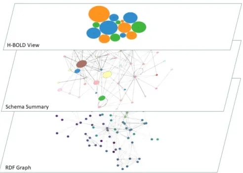
Figure 1:Example of different levels of the visual abstraction of a LOD source.
Data exploration and visualization systems are of great importance in the era of Big Data, where the volume and heterogeneity of the information available makes it difficult for the humans to explore and analyze data manually. Providing tools to view and explore large datasets has become a major research challenge.
From the point of view of the literature, different tools and techniques for navigation and visualization of linked data have been published [Bikakis and Sellis, 2016, Dadzie and Rowe, 2011, Marie and Gandon, 2014]. However, most of traditional LOD vi-sualization systems are limited to accessing small, static datasets that can easily be manipulated using conventional techniques. On the other hand, the current need is dy-namic, on-the-fly visualization of large datasets, integrated with efficient exploration techniques, as well as mechanisms for abstraction and summary.
There are several open data catalogs that list datasets available as Linked Data. Some popular examples are DataHub (formerly CKAN)3, the main catalog that now move to a commercial service, the EU Open Data Portal4that lists open data published by EU institutions and bodies free to use for commercial or non-commercial purposes, DataPortals5 that provides a comprehensive list of open data portals from around the
3
http://datahub.io
4http://data.europa.eu/euodp/en/home 5
world and several national or regional data portals (e.g. data.gov, data.gov.uk, etc.). There is not a single aggregation point. All these portals allow users to perform key-word search over their list of sources but do not provide analytics over the registered datasets and highly depends on the user input. These factors limit the possibility to obtain general insights into the LOD sources. The lack of such perception hinders im-portant data management tasks such as quality and coverage analysis. When a user starts exploring in details an unknown dataset, several issues arise: (1) the difficulty in finding documentation describing the source (often poor and sometimes missing); (2) the complexity of understanding the schema (since there are no fixed modeling rules); (3) the effort to explore a source with an extremely high number of instances; (4) the required skills of writing specific SPARQL queries.
This paper aims to overcome the above problems by providing the users with an incremental and multilevel visualization system to navigate LOD sources (our vision is shown in Figure 1). The H-BOLD tool neither requires a priori knowledge of the dataset nor particular user skills (like SPARQL knowledge). The billions of instances reported in a RDF dataset are grouped within a Schema Summary that shows only the classes of the LOD source. In case of a Big Linked Data, where also the number of classes is high, a clustering phase is add to grouped the classes in clusters, thus rendering a high-level view and enabling a incremental navigation of the dataset.
Starting from the URL of a SPARQL endpoint, H-BOLD exploits the query compu-tation power of the endpoint, without requiring any local materialization of the dataset, then it extracts statistical and structural information that create a Schema Summary of the dataset. After this, it applies community detection algorithms to create a high-level and compact view of the dataset.
Contributions.The main contributions of this paper are:
– a model for building, visualizing, and interacting with hierarchically organized Linked Open Data;
– a prototype system which implements the presented model and offers a two-level visual exploration and analysis over Linked Data of medium or big size;
– a test of the prototype on 126 Linked Data sources that expose a reachable SPARQL endpoint;
– a comparison of four community detection approaches for the hierarchical repre-sentation of Big Open Linked Data.
Outline.The remainder of this paper is organized as follows. Section 2 shows the architecture of H-BOLD. Here, a formal definition of the Schema Summary and Cluster Graph is introduced. A use case scenario is illustrated in Section 3. In Section 4, the effectiveness of H-BOLD on the LOD listed on DataHub is evaluated. Four algorithms for efficient community detection are presented and evaluated in Section 5. We discuss
related work in Section 6. In the end, Section 7 sketches the conclusion and the future lines of extension for H-BOLD.
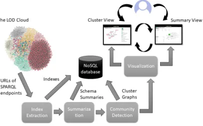
Figure 2:Architecture of H-BOLD.
2
H-BOLD
In this section, H-BOLD (High level visualizations on Big Open Linked Data), a tool for visualizing, and interacting with Big Linked Data is introduced.
H-BOLD is defined in the context of hierarchical visual exploration and analysis over LOD. H-BOLD starts from our past experience with the tool LODeX [Benedetti et al., 2015b, Benedetti et al., 2014b, Benedetti et al., 2014a, Benedetti et al., 2015a] and tried to overcome the main limitations arose during its evaluation [Benedetti et al., 2015c]. In particular, we want to avoid the visualization of complex graphs with more then 30 nodes (for an example of complex graph see Figure 5). In these cases, com-munity detection techniques in order to create a high-level visualization on the Schema Summary are applied and an high level graph is computed.
The architecture of H-BOLD is shown in Figure 2. The process of creating a high-level visualizations of BOLD is obtained in four sequential phases:
– Index Extraction; – Summarization; – Community Detection; – Visualization.
After a brief description of the extraction and the summarization, the paper will mainly focus on the community detection and the visualization components that have been heavily modified in H-BOLD. For more details on the Index Extraction please refers to [Benedetti et al., 2014a]. For an easy reuse, all the contents extracted and processed by H-BOLD are stored in MongoDB [Banker, 2011], a NoSQL document database, since it allows a flexible representation of the indexes.
2.1 Index Extraction
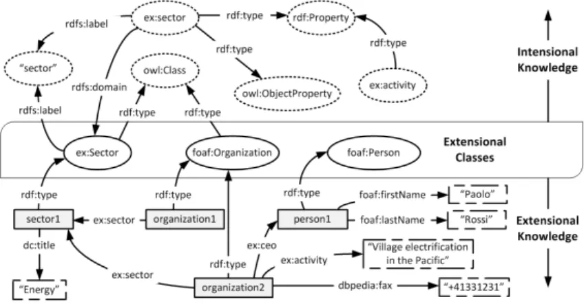
In a RDF graph the RDFS/OWL triples used to define a vocabulary or an ontology describe the intensional knowledge of the dataset, while the datatype and object prop-erties and the instances compose the extensional knowledge. In Figure 3 an example of the RDF graph representing a LOD source is displayed. The intensional knowledge is conveyed in the triples shown on the top of the figure, while, on the bottom, we have triples that describe three instances and compose the extensional knowledge. The In-dex Extraction takes as input the URL of a SPARQL endpoint and generates the set of queries needed to extract structural and statistical information from the LOD source. It is able to deal with the performance issues of the different implementations of SPARQL endpoints by usingpattern strategies.
Figure 3:An RDF graph partitioned between intensional and extensional knowledge.
These indexes are composed by statistical information (such as: number of triples, number of instances, number of instantiated classes, number of properties), the list of Classes and a series of couple (c,p), wherecis a class andpis a property, defined as in the following:
– SCl(Subject Class to literal) contains a list of datatype propertiespand their do-main classc;
– OC(Object Class) contains a list of object propertiespand their range classc. Table 1 lists the indexes extracted from the LOD source shown in Figure 3. The indexes are stored in the MongoDB and they are used to generate the Schema Summary [Benedetti et al., 2014a].
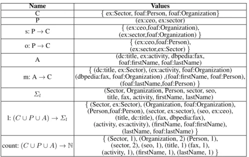
Table 1:Classes and indexes extracted from the source depicted in Figure 3
Name Values
Number of triples 12
Number of instances 4
Number of instantiated Classes 3
Number of property 8
Classes {ex:Sector, foaf:Person,foaf:Organization} SC {(foaf:Organization, ex:ceo), (foaf:Organization, ex:sector)} SCl {(foaf:Person, foaf:firstName), (foaf:Person, foaf:lastName), (ex:Sector,dc:title), (foaf:Organization, ex:activity), (foaf:Organization, dbpedia:fax)} OC {(ex:Sector,ex:sector), (foaf:Person, ex:ceo)} 2.2 Summarization
The Schema Summary of a LOD source is created by exploiting information contained in the indexes described in the previous section. The number of instances of each class and the number of times a index appear in a dataset are exploited in order to discover how the classes are connected in the extensional knowledge; thus, the Schema Summary is inferred from the distribution of the dataset instances. The formal definition is given below.
Definition 1 (Schema Summary) A Schema Summary S, derived from a RDF dataset, is a pseudograph:S=<C,P,s,o,A,m,Σl,l,count>, where:
– C contains a set of c, where c is a Class of the RDF dataset, the elements of C represent the node of the pseudograph;
– P contains the object properties, also called property, between Classes of the RDF dataset, the elements of P represent the edges of the pseudograph;
– o: P→C is a function that assigns to each property p∈P its object class c∈C;
– A contains the datatype properties, also called attribute, of the RDF dataset;
– m: A→C is a function that map each attribute a∈A to the class c∈C to which it refers.
– Σlis the finite alphabet of the available labels.
– l:(C∪P∪A)→Σlis function that assigns to each class, property or attribute
its label.
– count:(C∪P ∪A)→Nis a function that assigns to each property or attribute the number of times its appear in the LOD dataset, while if the input element is a class the output value represents the number of instances of the class.
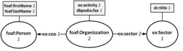
The Schema Summary offers several advantages: it can be easily memorized and re-trieved on the MongoDB improving data recovery performance and graph visualization. Table 2 reports the Schema Summary create on the previous RDF example of Figure 3, while Figure 4 depicts its graphical representation. Here, the white circles represents classes (C), while the attributes (A) are shown in the gray boxes. The edges represent one or more object properties (P). Each element is equipped with a numerical value representing the number of occurrences (or the number of instances for the classes).
Figure 4:Schema Summary generated from the source depicted in Figure 3.
2.3 Community Detection
The Schema Summary is a good approach to represent a RDF dataset in a compact way, however when we are dealing with big sources, it happens that the number of classes is high, thus the schema summary contains a high number of nodes and the visualization results complex and confused, as shown in the example of Figure 5. Realistically, the human brain can interpret at most a few dozen nodes in one graph when dealing with detail. Moreover, in a large connected dataset, the number of links increases exponen-tially with nodes. Eventually, this results in such a densely connected network that its beyond the help of any automated layout.
Table 2:Schema Summary of the source depicted in Figure 3.
Name Values
C {ex:Sector, foaf:Person, foaf:Organization}
P (ex:ceo, ex:sector)
s: P→C {(ex:ceo,foaf:Organization),
(ex:sector,foaf:Organization)}
o: P→C {(ex:ceo,foaf:Person),
(ex:sector,ex:Sector)}
A (dc:title, ex:activity, dbpedia:fax,foaf:firstName, foaf:lastName) m: A→C
{(dc:title, ex:Sector), (ex:activity, foaf:Organization) (dbpedia:fax, foaf:Organization) ,(foaf:firstName, foaf:Person),
(foaf:lastName,foaf:Person)} Σl (Sector, Organization, Person, sector, seo,title, fax, activity, firstName, lastName)
l:(C∪P∪A)→Σl
{(Sector, ex:Sector), (Organization, foaf:Organization), (Person,foaf:Person), (sector, ex:sector), (seo, ex:ceo),
(title, dc:title), (fax, dbpedia:fax), (activity, es:activity), (firstName, foaf:firstName),
(lastName, foaf:lastName)}
count:(C∪P∪A)→N
{(Sector, 1), (Organization, 2) (Person, 1), (sector, 2), (seo, 1), (title, 1) (fax, 1), (activity, 1), (firstName, 1), (lastName, 1)}
By analyzing the schema summaries produced by our previous tool, LODeX, an important feature has emerged: a high concentration of arcs within specific groups of nodes. This feature is called community structure[Girvan and Newman, 2002]. A com-munity structure (or cluster) is a subset of the graph in which the connections between nodes are very dense while the connections among these subsets within the entire graph are loose.
The problem of detecting communities within a network can be handled using com-munity detection algorithms. In the past, comcom-munity detection applied on graphs has been extensive analyzed [Fortunato, 2010, Malliaros and Vazirgiannis, 2013, Fortunato and Hric, 2016]. There is no a single definition accepted for describing a cluster (some-time called community) in a graph, and the variants used in the literature are numerous. These kinds of algorithms are typically based on the topology information of the graph and each algorithm usually optimizes over a particular function/property which it deems important.
Related to the graph connectivity, each cluster should be connected; it means that there should be several paths connecting each pair of nodes within the cluster. It is generally accepted that a subset of nodes forms a good cluster, if the induced sub-graph is dense, and there are few connections from the included nodes to the rest of the graph [Kannan et al., 2004]. Considering both the features of connectivity and density, a possible definition for a graph cluster could be a connected component or a maxi-mal clique[Bomze et al., 1999]. This is a sub-graph into which no node could be added without losing the clique property. On the other hand, it is not always clear that a node
Figure 5:Example of a complex schema summary for a big linked data source.
should be assigned only to a unique cluster. In some domains could be interesting that a node belongs to several clusters. In the clustering of the Schema Summary, the possi-bility that a node belongs to several clusters is avoided.
In the following, the formal definition of Cluster Graph is outlined.
Definition 2 (Cluster Graph) A Cluster Graph G, derived from a Schema Summary S, is a pseudograph: G =<L,K,s,Σb,b, S>, where:
– L contains a set of l, where l is a Cluster of Classes of S, the elements of L represent the node of the pseudograph;
– K contains the links between the clusters, the elements of K represent the edges of the pseudograph;
– s: L→C is a function that assigns to each cluster l∈L its source class c∈C where C is the set of classes of the RDF dataset contained in S; a cluster might be mapped to several classes;
– Σbis the finite alphabet of the available labels.
– b:(L)→Σbis function that assigns to each cluster l its label.
The label in the Cluster Graph are assigned based on the degree (the sum of in-degree and out-in-degree) of the classes (nodes) in the Schema Summary.
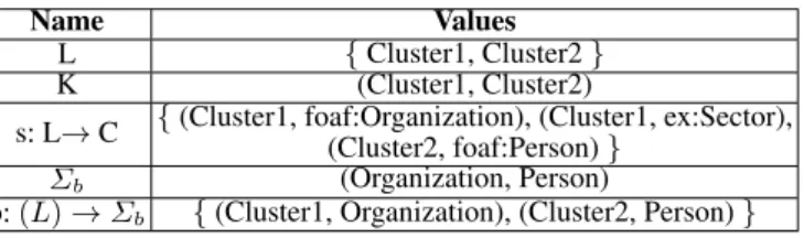
Table 3 reports the Cluster Graph that could be generated starting from the Schema Summary of Table 2/ Figure 4. Figure 6 depicts the graphical representation of the Clus-ter Graph. Here, it is possible to notice that the class “Person” is not grouped together
Figure 6:The Cluster Graph generated from the Schema Summary of Figure 4.
Table 3:Cluster Graph of the Schema Summary in Table 2.
Name Values
L {Cluster1, Cluster2}
K (Cluster1, Cluster2)
s: L→C {(Cluster1, foaf:Organization), (Cluster1, ex:Sector),(Cluster2, foaf:Person)}
Σb (Organization, Person)
b:(L)→Σb {(Cluster1, Organization), (Cluster2, Person)}
with other classes, while “Organization” and “Sector” are grouped in a unique cluster. This last cluster takes the name of “Organization” since it is the class with the higher degree in the cluster. The white circles represents clusters (L). The edges represent the connection between clusters (K).
2.4 Visualization
The visualization is organized in two levels:
– the higher level shows the Cluster View: here the clusters and their interconnections are displayed in an interactive graph; by selecting a cluster a list of the contained classes is shown, the selection of a set of classes is the pre-requisite to proceed to the next level of the visualization process;
– the second level shows a portion of the Schema Summary of the LOD source, here the classes that have been selected on the previous level are shown together with their properties and attributes. Iteratively, the graph can be expanded by adding new classes.
The visualization is performed by a web application through which the user can interact for browsing the Cluster View and the Schema View.
On the Schema View, the user might also define a visual query by selecting classes, properties and attribute. The process of the composition of a visual query has been extensively detailed in [Benedetti et al., 2015c].
The visualization module uses a MongoDb/Python backend. The GUI interface uses Data Driven Documents6[Bostock et al., 2011] and the Polymer library7to display and
6
http://d3js.org/
7
Figure 7:The overview panel of H-BOLD.
create the interactivity functions in the Cluster and Schema View.
3
A Use Case Scenario
An hypothetical use-case involving a lexical dataset, Dbnary, has been selected. Db-nary8provides multilingual lexical data extracted from wiktionary9. The extracted data is made available as Linguistic Linked Open Data. Linguistic data currently includes Bulgarian, Dutch, English, Finnish, French, German, Greek, Italian, Japanese, Polish, Portuguese, Russian, Serbo-Croat, Spanish, Swedish and Turkish.
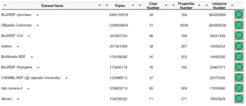
In the overview panel of H-BOLD [Po, 2018] (see Figure 7), we the SPARQL End-points are listed, the user can have, at a glance, the intuition of the dimension of the dataset. This dataset is composed of 140 millions of triples and contains around 33 mil-lions of instances. From the overview panel, the user selects to proceed to the Cluster View by clicking on the green button.
The Cluster View (see Figure 8) is a panel that represents the Cluster Graph as a network of nodes (clusters) link to each other by edges. By exploring this view, the user acquires the preliminary knowledge to undertake the navigation of the dataset. Indeed, the graph conveys the main topics of the source. In this case, the dataset is grouped in 5 clusters.
By selecting a node in the Cluster View, the list of classes that the cluster represents is shown on the left side (see Figure 9). The user is asked to select some classes in order to proceed to the next level of the visualization by clicking on the green button on the top right of the panel. In this particular case, we selected the cluster “Vocable” and then, the classes “Word” and “Translation”.
The next visualization level shows a portion of the Schema Summary (see Figure 10) that contains only the classes selected in the previous level and the directly
con-8
http://kaiko.getalp.org/about-dbnary/
Figure 8:The Cluster View of the Dbnary dataset.
Figure 9:The Cluster View of the Dbnary dataset with the“Vocable” node selected.
nected classes (other classes that are linked through an object property to the selected classes). In this case, starting from the selection of two classes (“Word” and “Transla-tion”), the displayed graph contains 11 nodes (classes). As shown on the bottom right of the panel, only a portion of the global Schema Summary is represented in the graph. In this case, it is the 30%. The user is now aware that he is navigating a portion of the classes of the dataset, he perceives the influence of each class by looking at its dimen-sion (that is proportional to the number of instances of the class) and its provenance (since the color of the nodes express to which vocabulary the class belongs to). In this case, “Translation” and “Vocable” are defined in the Dbnary vocabulary, while “Word” and “LexicalEntry” belongs to the Lemon vocabulary.
The user might iteratively expand the portion of the Schema Summary that is visu-alized by selecting additional classes. In the example, by double clicking on “Vocable”,
Figure 10:The Schema View of the 30% of the Dbnary dataset.
the graph is expanded with the classes directly connected to this node and a bigger graph is then displayed (see Figure 11).
Figure 11:The selection of the “Vocable” node in the Schema View.
4
Performance Evaluation
In order to evaluate the effectiveness of H-BOLD, the tool has been used to create the Schema Summary and the Cluster Graph of the LOD sources listed on DataHub. First, the effectiveness of the Indexes Extraction is assessed. After that, the performances of the generation of the Schema Summary and Cluster Graph has been analyzed, in order to consider the portability of the H-BOLD approach.
We make use of the SPARQL endpoint list available on the SPARQL ENDPOINTS STATUS10. Based on this list, the 45% (255/565) of the SPARQL Endpoints listed on DataHub.io were available. The 71% of them were compliant with all SPARQL 1.0 features and the 39% of them with all SPARQL 1.1 features. As depicted in Table 4, a
10
http://sparqles.ai.wu.ac.at/interoperability(last update performed on 29th July 2017)
lowest number of endpoints was reachable when we performed the test (on 26th Febru-ary 2018). After a careful analysis, we have assessed that this result is ascribable to the fact that the list provided by SPARQL ENDPOINTS STATUS has not been updated in the last 7 months and that the information currently available on Datahub are also limited, since the website has been transformed to a commercial service. The H-BOLD prototype has been evaluated on the entire set of the reachable SPARQL endpoints, i.e. 126 linked data sources. The Schema Summary has been created on 92 out of 126 sources. On 34 endpoints some problems arose such as transaction timed out, Endpoint internal error or service temporarily unavailable. Examining the 92 Schema Summary, not all these graphs have a complex and rich structure that necessitate applying com-munity detection algorithm. Only 32 datasets resulted to be represented by a Schema Summary of more than 30 nodes, for these datasets the community detection algorithm has been applied and the Cluster Graph has been created. The community detection en-countered no problems on the 32 big datasets: all 32 were grouped and the cluster graph displayed.
Table 4:Sparql Endpoint test comparison on 2014 and 2018
Test 2014 2018
Dataset URLs 559 565
Reachable datasets 302 126 Index Extraction completed 185 92
Schema Summary created 185 92 Schema Summary with more then 30 nodes - 32 Cluster Summary created - 32
Table 5:Comparison of four datasets
KEGG GENES Dbnary DBLP in RDF (L3S) DBpedia Commons Triples number 7,253,775,779 140,069,679 Error 137,427,503
Instance number 758,529,915 33,312,624 54939 34,174,539
Class number 21 70 6 62
Property number 110 207 25 5,455
Extraction Time 35 minutes 2 minutes Error 2 minutes
Number of nodes
in the Schema Summary 1 41 Error 34
Number of nodes
Cluster Graph - 5 Error 5
The heterogeneity on the implementation of the SPARQL endpoints is one of the most critical aspects and it dramatically affects the performances of the Indexes Ex-traction process. To highlight this issue, in Table 5, we compared the characteristics
of four datasets11: KEGG GENE (knowledge on the molecular interaction and reac-tion networks), Dbnary (wikireac-tionary data for several languages), DBLP in RDF (L3S) and DBpedia Commons (Wikimedia Commons). In terms of size and complexity the datasets are very similar, but the extraction time on the first dataset takes more than 10 times compared to the second and the forth. DBLP is a borderline case; although it is less complex than the other datasets, the extraction process has not been completed.
5
Community detection algorithm comparison
The following four algorithms for Community Detection has been compared and tested within the H-BOLD infrastructure:
– Edge betweenness proposed by Newman and Girvan in [Newman and Girvan, 2004a]
– Leading eigenvectorproposed by Newman in [Newman, 2006] – Louvaindefined by Blondel et al. [Blondel et al., 2008]
– Walktrapintroduced by Pons and Latapy [Pons and Latapy, 2005]
We make use of the library IGRAPH [Csardi and Nepusz, 2006] for the implementation of the algorithms. In the following, we introduce a short description for each of the algorithms and then we focus on the comparison performed on 32 Big Linked Data.
5.1 Edge Betweenness
The Edge-Betweenness [Newman and Girvan, 2004a] algorithm is a divisive hierarchi-cal algorithm that makes use of a top-down approach for the partition of the community graph. The algorithm starts from the assumption that, if two communities are united only by a few edges, all the paths that link the nodes of one community to another must necessarily pass for one of these edges. The algorithm then calculates the shortest paths, i.e. the shortest paths between all the vertex pairs and counts how many of these they cross each arch, consequently, the arch that will be crossed by the shortest path will also have the highest betweenness and will, therefore, be removed. The betweenness is recalculated with each removal of a single arc. In this way, better results are obtained at the expense of a greater computational cost.
11
The cost refers to an implementation on a portable machine (Operative System: Windows 7 -64 bit, RAM: 6 GB, number of processors: 1, number of cores: 2).
Table 6:Evaluation of Community Detection algorithms on 32 Big Linked Data.
EDGE BETWEENESS EIGENVECTOR LOUVAIN WALKTRAP
Dataset Name (listed in DataHub) C N CM CM>3 Qty ET CM CM>3 Qty Sim ET CM CM>3 Qty ET CM CM>3 Qty Sim ET
Semantic Web Conference Corpus 142 127 34 3 0,2 0,966 5 5 0,26 0,78 0,026 5 5 0,32 0,001 19 7 0,24 0,77 0,003
education.data.gov.uk 99 88 10 2 0,01 1,34 3 3 0,4 0,99 0,02 3 3 0,4 0,001 4 2 0,39 0,93 0,007
Linked Logainm 96 76 2 1 0,02 0,057 4 3 0,25 0,83 0,008 6 5 0,33 0 6 4 0,3 0,87 0,002
Alpine Ski Racers of Austria 94 79 9 5 0,55 0,18 10 5 0,54 0,79 0,027 11 7 0,59 0,001 11 6 0,62 0,74 0,003
Environment Agency Bathing Water Quality 93 81 14 5 0,44 0,18 11 7 0,42 0,65 0,048 7 6 0,49 0,001 10 7 0,42 0,69 0,002
kdata 90 73 37 5 0,25 0,38 11 8 0,28 0,71 0,046 6 5 0,39 0,001 6 4 0,3 0,71 0,003
Statistics Fatal Traffic Accidents Greek roads 89 48 7 5 0,5 0,004 7 6 0,57 0,98 0,008 7 6 0,58 0,001 9 6 0,56 0,96 0
Linked Open Financial Data 88 62 4 4 0,5 0,087 6 5 0,51 0,86 0,03 4 4 0,52 0 6 4 0,49 0,78 0,001
Open Data Thesaurus 86 80 8 4 0,54 0,12 10 6 0,61 0,81 0,026 11 7 0,63 0,001 11 6 0,62 0,87 0,002
Bio2RDF::Wormbase 86 49 5 4 0,39 0,016 4 3 0,34 0,76 0,008 5 4 0,39 0 4 3 0,39 0,94 0,001
data-artium-org 86 44 - - - - Error - - - - 7 5 0,63 1 0,014 7 5 0,63 0,001 6 4 0,61 0,95 0
dati.camera.it 85 54 23 2 0,29 0,036 7 7 0,37 0,69 0,02 6 6 0,45 0 6 4 0,37 0,71 0,001
World War 1 as Linked Open Data 84 70 7 6 0,47 0,091 7 5 0,4 0,7 0,081 7 7 0,5 0,001 8 5 0,45 0,79 0,002
data-szepmuveszeti-hu 83 44 9 4 0,58 0,008 7 5 0,64 0,9 0,009 8 4 0,65 0,001 5 3 0,57 0,9 0,001
Bio2RDF::Affymetrix 78 56 26 2 0,05 0,03 5 3 0,26 0,96 0,006 4 3 0,27 0,001 5 3 0,26 0,97 0,001
Bio2RDF::Ncbigene 76 48 26 2 0,1 0,064 5 4 0,31 0,88 0,02 4 3 0,33 0,001 7 4 0,27 0,81 0,002
Bio2RDF::Omim 75 46 3 2 0,11 0,032 7 3 0,19 0,76 0,01 5 3 0,26 0 9 4 0,2 0,76 0,001
Bio2RDF::Sabiork 74 53 3 2 0,1 0,02 7 3 0,35 0,73 0,015 7 6 0,4 0,001 7 4 0,35 0,75 0,001
Transparency International Linked Data 73 51 7 6 0,5 0,028 9 5 0,5 0,72 0,043 6 6 0,51 0 8 6 0,45 0,83 0,001
Linked Sensor Data (Kno.e.sis) 72 49 5 4 0,62 0,005 6 4 0,6 0,99 0,016 5 4 0,62 0 5 4 0,62 1 0,001
dbnary 71 37 - - - - Error - - - - 5 3 0,6 1 0,005 5 3 0,6 0 4 3 0,55 0,99 0
Bio2RDF::Interpro 70 48 15 2 0,19 0,022 4 3 0,29 0,76 0,009 5 4 0,35 0,001 5 3 0,28 0,83 0
Bio2RDF::Orphanet 69 38 4 3 0,52 0,005 6 3 0,49 0,83 0,007 5 4 0,54 0,001 4 3 0,52 0,91 0
UNESCO Institute for Statistics (UIS) 67 63 5 5 0,5 0,082 6 4 0,49 0,84 0,035 6 6 0,51 0,001 7 5 0,49 0,88 0,001
Bio2RDF::Ctd 66 38 5 4 0,38 0,015 6 5 0,36 0,76 0,019 5 4 0,39 0 8 5 0,34 0,79 0,001 webnmasunotraveler 66 35 5 3 0,28 0,008 5 5 0,32 0,8 0,017 5 4 0,35 0 5 4 0,35 0,83 0,001 ECLAP 63 44 6 2 0,05 0,13 6 4 0,45 0,93 0,02 6 4 0,48 0 8 5 0,4 0,8 0,001 Reactome RDF 62 39 12 3 0,2 0,028 5 3 0,28 0,83 0,009 6 4 0,33 0,001 6 3 0,28 0,73 0 Bio2RDF::Hgnc 61 32 3 2 0,33 0,003 4 3 0,39 0,91 0,005 4 3 0,4 0,001 3 2 0,33 0,83 0 Senato Italiano 54 32 6 4 0,59 0,002 7 4 0,56 0,8 0,01 6 4 0,6 0,001 8 4 0,57 0,88 0,001 reference.data.gov.uk 50 44 16 4 0,34 0,052 5 4 0,38 0,8 0,022 5 4 0,4 0 6 3 0,33 0,75 0,001 statistics.data.gov.uk 38 34 14 2 0,14 0,04 4 3 0,23 0,63 0,02 5 4 0,25 0 8 2 0,19 0,69 0,002
5.2 Leading eigenvector
This algorithm was theorized by Newman in 2006 [Newman, 2006], it is a top-down algorithm that makes use of the eigenvalues of a matrix called the modularity matrix. Initially, the partitioning of the graph is carried out in only two communities. The goal of the algorithm is to maximize the quality measure through the eigenvalues and eigen-vectors of the matrix. The algorithm looks for a set of autoeigen-vectors of the matrix to which the highest positive eigenvalue corresponds, by assigning the various nodes to the two communities according to the elements of the autovector. The procedure is repeated recursively until an increase in the quality of the partitioning is no longer possible.
5.3 Louvain
The Louvain approach [Blondel et al., 2008], also known as Multilevel, is a bottom-up hierarchical algorithm whose main objective is to maximize the quality of the commu-nity partition in a short time. The algorithm operates in two phases, first assigning each node to a different community, creating as many communities as nodes in the graph, after that, a node is chosen randomly and moved to the neighboring communities mea-suring the variation of quality from time to time. The node will then be assigned to the community for which the gain in quality is maximum or, if no gain is possible, the node will remain in its initial community. This procedure is repeated for all the nodes until the increase in quality is no longer possible. The second step is to consider the newly found communities as nodes of a new graph and proceed as in the first part. This algorithm has the advantage of being extremely simple and easy to be implemented. It also works quickly as the number of communities decreases at each iteration by concentrating the maximum workload only in the initial steps.
5.4 Walktrap
The Walktrap [Pons and Latapy, 2005] is an algorithm that exploits the concept of
random walksto form communities. Random walks tend to stay within a certain range community because the density of the internal edges is much greater of that of the edges that lead to the outside. The algorithm operates hierarchically from bottom to top, establishing an initial measure of distance to the nodes and then building a dendrogram based on the aforementioned measure. The algorithm works by posing each node into a different community, it calculates the distances between all the adjacent nodes and, in the end, aggregates two communities who have at least one edge that connects them. This procedure is repeatedn-1times, withnnumber of nodes, obtaining a hierarchical community in the form of a dendrogram. The communities to be merged are decided based on a methodology theorized by Ward in [Ward, 1963].
5.5 Evaluation
The lack of reliable gold-standard communities has made community detection a very challenging task [Yang and Leskovec, 2012], thus the evaluation of how good a set of community is it is difficult to score. In the running experiments (see Table 6), we have reported, for each of the four algorithms, the number of communities (CM), the number of communities with more then 3 elements (CM¿3), the quality of the communities (Qty) [Newman and Girvan, 2004b], the similarity within the communities (Sim) and the execution time in milliseconds (ET). The quality measure (Qty)12is a value assigned to each partition of the graph; the higher the value the better the partition.
The comparison has been execute on the Big Linked Data that have more then 30 classes, thus based on the numbers reported in table 4, on 32 datasets. The results of the evaluations are shown in Figure 6. The datasets can be retrieved by searching their names in Datahub13.
The Edge-Betweenness algorithm, the “older” one, has a high computational com-plexity ofO(nm2)wheremis the number of edges andnthe number of nodes, till O(n3)in case of a very little connected graph; this implies that the algorithm is suitable only for graphs of small dimensions, around the thousand of nodes. In our case, on the 32 examined graphs, the number of nodes is not so high. By applying this algorithm, we obtained a good average quality but the trend is not constant; in fact, for some graphs the results are good, while others have a quality that is close to 0. The number of com-munities found, in the case of graphs with more than 50 nodes, is higher then ten. All these problems lead to discard the algorithm of Girvan and Newman avoiding further analysis.
The Leading Eigenvector algorithm, although it has a high complexity equal to O((m+n)n) gave better results compared to the previous one, managing to main-tain a constant quality on all the graphs and a number of community always around ten or less, behaving good on medium-large size graph (30 to 50 nodes) and, also, on graph of larger sizes (more than 50 nodes), proving to be well adapted to the various graphs produced by H-BOLD.
The Walktrap algorithm has a complexity proportional to the heightHof the created dendrogram, equal toO(mnH), thus bringing the theoretical worst case toO(mn2)or O(n3)ifm =nwhich does not allow scalability. However, according to the authors, most real networks are not highly connected and their dendrogram is balanced with a small height. In this ideal condition, the general complexity becomesO(n2logn), which still remains quite high. Nevertheless in the tests carried out, the execution times were excellent, clearly outclassing from the Edge-Betweenness algorithm with which it shares a similar complexity. The Walktrap manages to obtain a fairly constant quality.
12
This measure is based on the hypothesis that a random graph, that is a graph where the edges connecting the nodes are randomly chosen, do not have a community structure. The quality measure compares the number of edges present in a certain cluster with that expected if the graph did not have a community structure.
13
The Louvain algorithm is probably the simplest from the implementation point of view among all the others. It has a linear computational complexity, which makes it ex-tremely scalable as also evidenced in [Blondel et al., 2008]. In [Yang et al., 2015], the Louvain algorithm was compared to all the algorithms here analyzed, demonstrating how this manages to process large amounts of data in far less time than competitors, while maintaining high levels of accuracy. In the tests carried out on H-BOLD, the al-gorithm managed to obtain an average quality around 0,45, creating a very low number of communities in every type of graph in which it has been applied, which makes it the candidate ideal for the community partition for H-BOLD graphs.
6
Related Work
H-BOLD aims to produce a synthetic multilevel view of an RDF dataset to support users in the exploration of LOD, therefore his algorithms and techniques overlap with different research topics in the field of semantic web. These topics encompass: visu-alization and documentation of LOD sources, semantic index extraction and schema summarization.
Most exploration and visualization systems that deal with LOD do not handle per-formance and scalability problems, but use traditional techniques to manage small data sets. In LOD, visualization systems can be divided into generic systems and graph-oriented systems. Generic display systems (such as Rhizomer [Brunetti et al., 2012], LODWheel[Stuhr et al., 2011], SemLens [Heim et al., 2011], Payola [Kl´ımek et al., 2013], LDVizWiz [Atemezing and Troncy, 2014], VisWizard [Tschinkel et al., 2014], LinkDaViz [Thellmann et al., 2015], ViCoMap [Ristoski and Paulheim, 2015]) support different types of data (for example, numbers, temporal, graphical, spatial) and pro-vide different types of visualization. Some systems offer recommendation mechanisms suggesting the most suitable form of visualization depending on the input data (Link-DaViz, VisWizard, LDVizWiz). Graph-oriented system (such as FlexViz web applica-tions [Falconer et al., 2010], RelFinder [Heim et al., 2010], Lodlive [Camarda et al., 2012], VOWL 2 [Lohmann et al., 2016], graphVizdb [Bikakis et al., 2016]) are of great importance due to the graphical structure of the RDF data model. Although several sys-tems offer sampling or aggregation mechanisms, most of these load the entire graph into central memory. Because graph layout algorithms require a lot of memory to draw large graphs, current systems are limited to handling small graphs. With regard to vi-sual scalability, most systems do not adopt approximation techniques such as sampling, filtering or aggregation. Existing approaches assume that all objects can be presented on the screen and managed through traditional visualization techniques, thus limiting their applicability to data sets of limited size. Exceptions in this scenario are the cases of SynopsViz14[Bikakis et al., 2017] and VizBoard [Voigt et al., 2012] which exploit external memory at runtime. And also GrouseFlocks [Archambault et al., 2008] is a
system for the exploration of a graph hierarchy space. By allowing users to see sev-eral different possible hierarchies on the same graph, the system helps users investigate graph hierarchy space instead of a single fixed hierarchy.
In order to handle large graphs, modern systems should adopt more sophisticated techniques such as:
– use hierarchical aggregation approaches in which the graph is recursively decom-posed into smaller subgroups (using clustering and partitioning techniques), form-ing a hierarchy of levels of abstraction [Archambault et al., 2008, Auber, 2004, Ro-drigues et al., 2013, Li et al., 2015];
– adopt edge grouping techniques that aggregate the edges of the graph into bundles [Cui et al., 2008, Gansner et al., 2011];
– consider scalability and performance as key requirements and deepen disk-based implementations, as in [Rodrigues et al., 2006, Sundara et al., 2010].
7
Conclusion & Future Works
In this paper, a tool for multilevel visual exploration of Big Linked Data has been pre-sented.
H-BOLD extends our previous tool LODeX and provides users with an interac-tive GUI that makes possible the exploration of billions of instances reported in a RDF dataset. The application of community detection algorithms allows to explore Big datasets. By selecting a set of classes from one of the clusters that represent the LOD, it is possible to explore the classes, attributes and properties and incrementally adding new ones enabling a incremental navigation of the dataset. This tool facilitates users’ interaction with LOD sources, making more pleasant the consumption of Linked Data without requiring any a priori knowledge of the dataset nor any SPARQL skills. H-BOLD has been tested on 32 Big Linked Data showing good performances.
In the next future, we hope to evaluate the effectiveness of H-BOLD as a visualiza-tion tool through a user study involving different kind of LOD consumers (practivisualiza-tioners, unskilled users, domain experts). It may also be interesting to experiment with hierar-chical clustering algorithms such as the agglomerative algorithms (bottom-up approach) and the divisive algorithms (top-down approach).
8
Acknowledgement
This work has been partially supported by the “H-BOLD: Building high level visual-izations on Big Open Linked Data” project funded by the “Enzo Ferrari” Engineering Department of the University of Modena and Reggio Emilia within FAR2017.
References
[Archambault et al., 2008] Archambault, D., Munzner, T., and Auber, D. (2008). Grouseflocks: Steerable exploration of graph hierarchy space.IEEE Transactions on Visualization and Com-puter Graphics, 14(4):900–913.
[Atemezing and Troncy, 2014] Atemezing, G. A. and Troncy, R. (2014). Towards a linked-data based visualization wizard. InProceedings of the 5th International Conference on Consum-ing Linked Data - Volume 1264, COLD’14, pages 1–12, Aachen, Germany, Germany. CEUR-WS.org.
[Auber, 2004] Auber, D. (2004). Tulip — a huge graph visualization framework. In J¨unger, M. and Mutzel, P., editors,Graph Drawing Software, pages 105–126. Springer Berlin Heidelberg, Berlin, Heidelberg.
[Baker and Keizer, 2010] Baker, T. and Keizer, J. (2010). Linked data for fighting global hunger: experiences in setting standards for agricultural information management. InLinking enter-prise data, pages 177–201. Springer.
[Banker, 2011] Banker, K. (2011).MongoDB in action. Manning Publications Co.
[Barnaghi et al., 2010] Barnaghi, P., Presser, M., and Moessner, K. (2010). Publishing linked sensor data. InCEUR Workshop Proceedings: Proceedings of the 3rd International Workshop on Semantic Sensor Networks (SSN), Organised in conjunction with the International Semantic Web Conference, volume 668.
[Benedetti et al., 2014a] Benedetti, F., Bergamaschi, S., and Po, L. (2014a). Online index ex-traction from linked open data sources. InProceedings of the 2nd International Workshop on Linked Data for Information Extraction (LD4IE 2014) co-located with the 13th International Semantic Web Conference (ISWC 2014), Riva del Garda, Italy, October 20, 2014., pages 9–20. [Benedetti et al., 2015a] Benedetti, F., Bergamaschi, S., and Po, L. (2015a). Exposing the un-derlying schema of LOD sources. InIEEE/WIC/ACM International Conference on Web Intelligence and Intelligent Agent Technology, WIIAT 2015, Singapore, December 69, 2015 -Volume I, pages 301–304. IEEE Computer Society.
[Benedetti et al., 2015b] Benedetti, F., Bergamaschi, S., and Po, L. (2015b). Lodex: A tool for visual querying linked open data. In Villata, S., Pan, J. Z., and Dragoni, M., editors, Proceed-ings of the ISWC 2015 Posters & Demonstrations Track co-located with the 14th International Semantic Web Conference (ISWC-2015), Bethlehem, PA, USA, October 11, 2015., volume 1486 ofCEUR Workshop Proceedings. CEUR-WS.org.
[Benedetti et al., 2015c] Benedetti, F., Bergamaschi, S., and Po, L. (2015c). Visual querying LOD sources with lodex. InProceedings of the 8th International Conference on Knowledge Capture, K-CAP 2015, Palisades, NY, USA, October 7-10, 2015, pages 12:1–12:8.
[Benedetti et al., 2014b] Benedetti, F., Po, L., and Bergamaschi, S. (2014b). A visual summary for linked open data sources. InProceedings of the International Semantic Web Conference ISWC 2014 Posters & Demo Track, Riva del Garda, Italy, October 21, 2014., pages 173–176. [Beneventano et al., 2015] Beneventano, D., Bergamaschi, S., Gagliardelli, L., and Po, L.
(2015). Driving innovation in youth policies with open data. In Fred, A. L. N., Dietz, J. L. G., Aveiro, D., Liu, K., and Filipe, J., editors,Knowledge Discovery, Knowledge Engineering and Knowledge Management - 7th International Joint Conference, IC3K 2015, Lisbon, Portugal, November 12-14, 2015, Revised Selected Papers, volume 631 ofCommunications in Computer and Information Science, pages 324–344. Springer.
[Bikakis et al., 2016] Bikakis, N., Liagouris, J., Krommyda, M., Papastefanatos, G., and Sellis, T. K. (2016). graphvizdb: A scalable platform for interactive large graph visualization. In32nd IEEE International Conference on Data Engineering, ICDE 2016, Helsinki, Finland, May 16-20, 2016, pages 1342–1345. IEEE Computer Society.
[Bikakis et al., 2017] Bikakis, N., Papastefanatos, G., Skourla, M., and Sellis, T. (2017). A hi-erarchical aggregation framework for efficient multilevel visual exploration and analysis. Se-mantic Web, 8(1):139–179.
[Bikakis and Sellis, 2016] Bikakis, N. and Sellis, T. K. (2016). Exploration and visualization in the web of big linked data: A survey of the state of the art. In Palpanas, T. and Stefanidis, K., editors,Proceedings of the Workshops of the EDBT/ICDT 2016 Joint Conference, EDBT/ICDT
Workshops 2016, Bordeaux, France, March 15, 2016., volume 1558 ofCEUR Workshop Pro-ceedings. CEUR-WS.org.
[Blondel et al., 2008] Blondel, V. D., Guillaume, J.-L., Lambiotte, R., and Lefebvre, E. (2008). Fast unfolding of communities in large networks.Journal of Statistical Mechanics: Theory and Experiment, 2008(10):P10008.
[Bomze et al., 1999] Bomze, I. M., Budinich, M., Pardalos, P. M., and Pelillo, M. (1999). The maximum clique problem. In Du, D.-Z. and Pardalos, P. M., editors,Handbook of Combinato-rial Optimization: Supplement Volume A, pages 1–74. Springer US, Boston, MA.
[Bostock et al., 2011] Bostock, M., Ogievetsky, V., and Heer, J. (2011). D3 data-driven docu-ments.IEEE Transactions on Visualization and Computer Graphics, 17(12):2301–2309. [Brunetti et al., 2012] Brunetti, J. M., Auer, S., and Garca, R. (2012). The linked data
visualiza-tion model. InInternational Semantic Web Conference (Posters & Demos).
[Camarda et al., 2012] Camarda, D. V., Mazzini, S., and Antonuccio, A. (2012). Lodlive, ex-ploring the web of data. In Presutti, V. and Pinto, H. S., editors,I-SEMANTICS 2012 - 8th International Conference on Semantic Systems, I-SEMANTICS ’12, Graz, Austria, September 5-7, 2012, pages 197–200. ACM.
[Colacino and Po, 2017] Colacino, V. G. and Po, L. (2017). Managing road safety through the use of linked data and heat maps. In Akerkar, R., Cuzzocrea, A., Cao, J., and Hacid, M., editors,
Proceedings of the 7th International Conference on Web Intelligence, Mining and Semantics, WIMS 2017, Amantea, Italy, June 19-22, 2017, pages 18:1–18:8. ACM.
[Csardi and Nepusz, 2006] Csardi, G. and Nepusz, T. (2006). The igraph Software Package for Complex Network Research.InterJournal, Complex Systems:1695.
[Cui et al., 2008] Cui, W., Zhou, H., Qu, H., Wong, P. C., and Li, X. (2008). Geometry-based edge clustering for graph visualization.IEEE Trans. Vis. Comput. Graph., 14(6):1277–1284. [Dadzie and Rowe, 2011] Dadzie, A.-S. and Rowe, M. (2011). Approaches to visualising linked
data: A survey.Semant. web, 2(2):89–124.
[Ding et al., 2012] Ding, L., Peristeras, V., and Hausenblas, M. (2012). Linked open government data [guest editors’ introduction].Intelligent Systems, IEEE, 27(3):11–15.
[Falconer et al., 2010] Falconer, S. M., Callendar, C., and Storey, M. D. (2010). A visualization service for the semantic web. In Cimiano, P. and Pinto, H. S., editors,Knowledge Engineering and Management by the Masses - 17th International Conference, EKAW 2010, Lisbon, Portu-gal, October 11-15, 2010. Proceedings, volume 6317 ofLecture Notes in Computer Science, pages 554–564. Springer.
[Fortunato, 2010] Fortunato, S. (2010). Community detection in graphs. Physics Reports, 486(3):75 – 174.
[Fortunato and Hric, 2016] Fortunato, S. and Hric, D. (2016). Community detection in net-works: A user guide. Physics Reports, 659:1 – 44. Community detection in networks: A user guide.
[Gansner et al., 2011] Gansner, E. R., Hu, Y., North, S. C., and Scheidegger, C. E. (2011). Mul-tilevel agglomerative edge bundling for visualizing large graphs. In Battista, G. D., Fekete, J., and Qu, H., editors,IEEE Pacific Visualization Symposium, PacificVis 2011, Hong Kong, China, 1-4 March, 2011, pages 187–194. IEEE Computer Society.
[Girvan and Newman, 2002] Girvan, M. and Newman, M. E. J. (2002). Community structure in social and biological networks.PNAS, 99(12):7821–7826.
[Heim et al., 2010] Heim, P., Lohmann, S., and Stegemann, T. (2010). Interactive relationship discovery via the semantic web. In Aroyo, L., Antoniou, G., Hyv¨onen, E., ten Teije, A., Stuck-enschmidt, H., Cabral, L., and Tudorache, T., editors,The Semantic Web: Research and Appli-cations, 7th Extended Semantic Web Conference, ESWC 2010, Heraklion, Crete, Greece, May 30 - June 3, 2010, Proceedings, Part I, volume 6088 ofLecture Notes in Computer Science, pages 303–317. Springer.
[Heim et al., 2011] Heim, P., Lohmann, S., Tsendragchaa, D., and Ertl, T. (2011). Semlens: vi-sual analysis of semantic data with scatter plots and semantic lenses. In Ghidini, C., Ngomo, A. N., Lindstaedt, S. N., and Pellegrini, T., editors,Proceedings the 7th International Confer-ence on Semantic Systems, I-SEMANTICS 2011, Graz, Austria, September 7-9, 2011, ACM International Conference Proceeding Series, pages 175–178. ACM.
[H¨ochtl and Reichst¨adter, 2011] H¨ochtl, J. and Reichst¨adter, P. (2011). Linked open data -A means for public sector information management. In -Andersen, K. N., Francesconi, E., Gr¨onlund, ˚A., and van Engers, T. M., editors,Electronic Government and the Information Sys-tems Perspective - Second International Conference, EGOVIS 2011, Toulouse, France, August 29 - September 2, 2011. Proceedings, volume 6866 ofLecture Notes in Computer Science, pages 330–343. Springer.
[Hyv¨onen, 2012] Hyv¨onen, E. (2012). Publishing and using cultural heritage linked data on the semantic web.Synthesis Lectures on the Semantic Web: Theory and Technology, 2(1):1–159. [Jupp et al., 2014] Jupp, S., Malone, J., Bolleman, J., Brandizi, M., Davies, M., Garcia, L.,
Gaulton, A., Gehant, S., Laibe, C., Redaschi, N., et al. (2014). The ebi rdf platform: linked open data for the life sciences.Bioinformatics, 30(9):1338–1339.
[Kannan et al., 2004] Kannan, R., Vempala, S., and Vetta, A. (2004). On clusterings: Good, bad and spectral.J. ACM, 51(3):497–515.
[Kl´ımek et al., 2013] Kl´ımek, J., Helmich, J., and Necask´y, M. (2013). Payola: Collaborative linked data analysis and visualization framework. In Cimiano, P., Fern´andez, M., L´opez, V., Schlobach, S., and V¨olker, J., editors,The Semantic Web: ESWC 2013 Satellite Events - ESWC 2013 Satellite Events, Montpellier, France, May 26-30, 2013, Revised Selected Papers, volume 7955 ofLecture Notes in Computer Science, pages 147–151. Springer.
[Li et al., 2015] Li, C., Baciu, G., and Wang, Y. (2015). Modulgraph: modularity-based visu-alization of massive graphs. InSIGGRAPH Asia 2015 Visualization in High Performance Computing, Kobe, Japan, November 2-6, 2015, pages 11:1–11:4. ACM.
[Lohmann et al., 2016] Lohmann, S., Negru, S., Haag, F., and Ertl, T. (2016). Visualizing on-tologies with VOWL.Semantic Web, 7(4):399–419.
[Malliaros and Vazirgiannis, 2013] Malliaros, F. D. and Vazirgiannis, M. (2013). Clustering and community detection in directed networks: A survey.Physics Reports, 533(4):95 – 142. Clus-tering and Community Detection in Directed Networks: A Survey.
[Marie and Gandon, 2014] Marie, N. and Gandon, F. (2014). Survey of linked data based explo-ration systems. InProceedings of the 3rd International Conference on Intelligent Exploration of Semantic Data - Volume 1279, IESD’14, pages 66–77, Aachen, Germany, Germany. CEUR-WS.org.
[Nesi et al., 2017] Nesi, P., Po, L., Viqueira, J. R. R., and Lado, R. T. (2017). An integrated smart city platform. In Szymanski, J. and Velegrakis, Y., editors,Semantic Keyword-Based Search on Structured Data Sources - Third International KEYSTONE Conference, IKC 2017, Gda´nsk, Poland, September 11-12, 2017, Revised Selected Papers and COST Action IC1302 Reports, volume 10546 ofLecture Notes in Computer Science, pages 171–176. Springer. [Newman, 2006] Newman, M. E. (2006). Finding community structure in networks using the
eigenvectors of matrices.Physical review E, 74(3):036104.
[Newman and Girvan, 2004a] Newman, M. E. J. and Girvan, M. (2004a). Finding and evaluat-ing community structure in networks.Physical Review, E 69(026113).
[Newman and Girvan, 2004b] Newman, M. E. J. and Girvan, M. (2004b). Finding and evaluat-ing community structure in networks.Phys. Rev. E, 69(2):026113.
[Po, 2018] Po, L. (2018). High-level visualization over big linked data. In van Erp, M., Atre, M., L´opez, V., Srinivas, K., and Fortuna, C., editors,Proceedings of the ISWC 2018 Posters & Demonstrations, Industry and Blue Sky Ideas Tracks co-located with 17th International Se-mantic Web Conference (ISWC 2018), Monterey, USA, October 8th - to - 12th, 2018., volume 2180 ofCEUR Workshop Proceedings. CEUR-WS.org.
[Pons and Latapy, 2005] Pons, P. and Latapy, M. (2005). Computing communities in large net-works using random walks. In Yolum, p., G¨ung¨or, T., G¨urgen, F., and ¨Ozturan, C., editors,
Computer and Information Sciences - ISCIS 2005: 20th International Symposium, Istanbul, Turkey, October 26-28, 2005. Proceedings, pages 284–293. Springer Berlin Heidelberg, Berlin, Heidelberg.
[Ristoski and Paulheim, 2015] Ristoski, P. and Paulheim, H. (2015). Visual analysis of statis-tical data on maps using linked open data. In Gandon, F., Gu´eret, C., Villata, S., Breslin, J. G., Faron-Zucker, C., and Zimmermann, A., editors,The Semantic Web: ESWC 2015 Satel-lite Events - ESWC 2015 SatelSatel-lite Events Portoroˇz, Slovenia, May 31 - June 4, 2015, Revised
Selected Papers, volume 9341 ofLecture Notes in Computer Science, pages 138–143. Springer. [Rodrigues et al., 2013] Rodrigues, J. F., Tong, H., Pan, J., Traina, A. J. M., Jr., C. T., and Faloutsos, C. (2013). Large graph analysis in the gmine system. IEEE Trans. Knowl. Data Eng., 25(1):106–118.
[Rodrigues et al., 2006] Rodrigues, J. F., Tong, H., Traina, A. J. M., Faloutsos, C., and Leskovec, J. (2006). Gmine: A system for scalable, interactive graph visualization and min-ing. In Dayal, U., Whang, K., Lomet, D. B., Alonso, G., Lohman, G. M., Kersten, M. L., Cha, S. K., and Kim, Y., editors,Proceedings of the 32nd International Conference on Very Large Data Bases, Seoul, Korea, September 12-15, 2006, pages 1195–1198. ACM.
[Rubin et al., 2008] Rubin, D. L., Moreira, D. A., Kanjamala, P., and Musen, M. A. (2008). Bioportal: A web portal to biomedical ontologies. InAAAI Spring Symposium: Symbiotic Re-lationships between Semantic Web and Knowledge Engineering, pages 74–77.
[Stuhr et al., 2011] Stuhr, M., Roman, D., and Norheim, D. (2011). Lodwheel - javascript-based visualization of RDF data. In Hartig, O., Harth, A., and Sequeda, J. F., editors,Proceedings of the Second International Workshop on Consuming Linked Data (COLD2011), Bonn, Germany, October 23, 2011, volume 782 ofCEUR Workshop Proceedings. CEUR-WS.org.
[Sundara et al., 2010] Sundara, S., Atre, M., Kolovski, V., Das, S., Wu, Z., Chong, E. I., and Srinivasan, J. (2010). Visualizing large-scale RDF data using subsets, summaries, and sam-pling in oracle. In Li, F., Moro, M. M., Ghandeharizadeh, S., Haritsa, J. R., Weikum, G., Carey, M. J., Casati, F., Chang, E. Y., Manolescu, I., Mehrotra, S., Dayal, U., and Tsotras, V. J., editors,Proceedings of the 26th International Conference on Data Engineering, ICDE 2010, March 1-6, 2010, Long Beach, California, USA, pages 1048–1059. IEEE Computer Society. [Thellmann et al., 2015] Thellmann, K., Galkin, M., Orlandi, F., and Auer, S. (2015).
Link-daviz - automatic binding of linked data to visualizations. In Arenas, M., Corcho, ´O., Sim-perl, E., Strohmaier, M., d’Aquin, M., Srinivas, K., Groth, P. T., Dumontier, M., Heflin, J., Thirunarayan, K., and Staab, S., editors,The Semantic Web - ISWC 2015 - 14th International Semantic Web Conference, Bethlehem, PA, USA, October 11-15, 2015, Proceedings, Part I, volume 9366 ofLecture Notes in Computer Science, pages 147–162. Springer.
[Tschinkel et al., 2014] Tschinkel, G., Veas, E. E., Mutlu, B., and Sabol, V. (2014). Using se-mantics for interactive visual analysis of linked open data. In Horridge, M., Rospocher, M., and van Ossenbruggen, J., editors,Proceedings of the ISWC 2014 Posters & Demonstrations Track a track within the 13th International Semantic Web Conference, ISWC 2014, Riva del Garda, Italy, October 21, 2014., volume 1272 ofCEUR Workshop Proceedings, pages 133– 136. CEUR-WS.org.
[Voigt et al., 2012] Voigt, M., Pietschmann, S., Grammel, L., and Meiner, K. (2012). Context-aware recommendation of visualization components. InProceedings of the 4th International Conference on Information, Process, and Knowledge Management eKNOW 2012, Valencia, Spain, January 30 - February 4, 2012, volume 2. IARIA XPS Press.
[Ward, 1963] Ward, J. H. (1963). Hierarchical grouping to optimize an objective function. Jour-nal of the American Statistical Association, 58(301):236–244.
[Yang and Leskovec, 2012] Yang, J. and Leskovec, J. (2012). Defining and evaluating network communities based on ground-truth. In2012 IEEE 12th International Conference on Data Mining, pages 745–754.
[Yang et al., 2015] Yang, Z., Algesheimer, R., and Tessone, C. (2015). A comparative analysis of community detection algorithms on artificial networks.Scientific Reports, 6.
![Table 1 lists the indexes extracted from the LOD source shown in Figure 3. The indexes are stored in the MongoDB and they are used to generate the Schema Summary [Benedetti et al., 2014a].](https://thumb-us.123doks.com/thumbv2/123dok_us/787155.2599525/6.892.277.647.368.594/indexes-extracted-figure-indexes-mongodb-generate-summary-benedetti.webp)