P-ISSN: 2087-2046; E-ISSN: 2476-9223 Page 301– 318
Measuring Systemic Risk of Banking in Indonesia: Conditional Value at Risk Model Application
Harjum Muharam1, Erwin2
Universitas Diponegoro
1[email protected], 2[email protected]
Abstract
Systemic risk is a risk of collapse of the financial system that would cause the financial system is not functioning properly. Measurement of systemic risk in the financial institutions, especially banks are crucial, because banks are highly vulnerable to financial crisis. In this study, to estimate the conditional value-at-risk (CoVaR) used quantile regression. Samples in this study of 9 banks have total assets of
the largest in Indonesia. Testing the correlation between VaR and ΔCoVaR in this study using
Spearman correlation and Kendall's Tau. There are five banks that have a significant correlation
between VaR and ΔCoVaR, meanwhile four others banks in the sample did not have a significant
correlation. However, the correlation coefficient is below 0.50, which indicates that there is a weak correlation between VaR and CoVaR.
Keywords: systemic risk, conditional value at risk, value at risk, banking industry Abstrak
Risiko sistemik adalah risiko jatuhnya sistem keuangan yang akan menyebabkan sistem keuangan tidak berfungsi dengan baik. Pengukuran risiko sistemik di lembaga keuangan terutama bank sangat penting, karena bank sangat rentan terhadap krisis keuangan. Dalam penelitian ini, untuk memperkirakan nilai kondisional-risiko (CoVaR) menggunakan regresi quantile. Sampel dalam penelitian terhadap 9 bank ini memiliki total aset terbesar di Indonesia. Menguji korelasi antara VaR
dan ΔCoVaR dalam penelitian ini dengan menggunakan korelasi Spearman dan Kendall's Tau. Ada
lima bank yang memiliki korelasi signifikan antara VaR dan ΔCoVaR, sedangkan empat bank lain
dalam sampel tersebut tidak memiliki korelasi yang signifikan. Namun, koefisien korelasi di bawah 0,50, yang mengindikasikan bahwa terdapat korelasi yang lemah antara VaR dan CoVaR.
Kata Kunci: risiko sistemik, conditional value at risk, value at risk, industri perbankan. Received: April 18, 2017; Revised: June 10, 2017; Approved: June 25, 2017
INTRODUCTION
In main function, the banks collect funds from surplus units and invest to deficit units in the form of loans and other financial instruments. Casu, et.al (2006) defined the bank is an intermediary institution that bridges the gap between lender and borrower to perform the functions of transformation, namely transformation size, maturity transformation and risk transformation. As a financial intermediary, the banking industry may be the highest vulnerable to financial risk. The functions are causes of vulnerability as a result of the bank's activities. This condition causes the banks face the risk of maturity mismatch are vulnerable to the threat of a bank run, namely withdrawals massive panic caused by customer. Besides the risk of maturity mismatch, other lines of bank business also cause the vulnerability of banks.
The main income of banks is difference between interest loans to creditors with interest given by banks to customers. But the bank also has other sources of income in the form of profit foreign exchange trading and securities. From this source of income, there is a gap that can lead to bank failures, when a decline in asset values as well as the increased uncertainty in the financial sector that have a negative effect on the activity of bank's operations. A systemic financial crisis will have an impact if many banks that have failed. The failure of one bank can propagate such as infectious diseases, causing more bank failures. If a bank failure or crisis cannot be dealt with swiftly, then there will be contagion effects that would trigger a systemic crisis in the economic system.
Systemic risk is defined as the potential instability due to interference transmitted in some or all of the financial system due to the interaction of size, business complexity and interconnectedness between institutions and/or financial markets as well as the tendency of excessive behavior from the behavior/financial institutions to follow the economic cycle (Bank of Indonesia, 2014). Systemic risk could be a polemic in Indonesia when the Financial System Stability Committee poured huge funds to rescue Bank Century (renamed Bank of Mutiara and later became J-Trust Bank). The recent financial crisis revealed that micro-prudential regulatory framework is not enough to prevent contagion across the world as a result of bank failures that began in the United States and later in Europe and other parts of the world, including in Indonesia.
Micro-prudential regulatory framework is based on the provisions of Basel I and II agreements, which impose minimum capital requirement (Capital Adequacy Ratio/CAR) as a preventive measure against unexpected losses (Pillar I). Drakos and Kouretas (2014) revealed that the Basel II agreements led to the development of internal systems for measuring market risk and regulation as viewed soundness of individual financial institutions. However, these provisions only based on capital adequacy ignore factors such as size, level of leverage, and the relationship with the entire system. Arnold et.al. (2012) found the key aspects of the new regulatory reforms through the Basel III agreement, including measurement and regulate systemic risk, as well as designing and implementing macro-prudential policies in a proper way. Basel III agreement is still in formation is expected to address most of the problems associated with systemic risk and developing an appropriate framework for regulation and supervision of financial markets. For central banks and financial regulators, this is a great value to be able to measure the risks that could threaten the financial system, not only at national level but also globally. Given the magnitude of losses incurred as a result of a systemic crisis, this study measures the level of systemic risk in the financial system in Indonesia, with a focus on banking institutions.
Assessing the level of systemic risk has gotten a lot of attention after the US financial crisis in 2007-2008. The main points of the issue of systemic risk is that the bank is experiencing distress will create panic in the financial system during periods of distress, causing the failure of other institutions and lead to the financial crisis. The most common measurement tool used by financial institutions in measuring the risk is value-at-risk (VaR), which was introduced by Jorion (2006). VaR is used to calculate possible losses of financial institutions within a certain confidence level. The problem that arises is that VaR does not consider the institution as part of a system that may be able to experience instability and spreading economic risks. Furthermore, it is known that the assessment focuses on information bank balance sheets, including the ratio of non-performing loan (NPL), earnings and profitability, liquidity and size of capital adequacy is not appropriate to evaluate the health of the financial system (Huang, et.al, 2009; Benoit, et.al, 2013).
Systemic risk contained in any system that is built by the components interacts with each other. A systemic risk said to be due to such risks arising from the
interaction of the unpredictability of the various components of the system. Systemic risk is known very widely, not only in the financial sector, but also in the medical field. Illustrations of these risks such as disease epidemics, i.e. an infectious disease outbreak quickly over a large area and caused many casualties. Systemic risk is a peculiarity of the financial system. Systemic crises can cause great harm in the real sector and the welfare state as a whole.
De-Bandt and Hartmann (2000) define a systemic event in the narrow sense as an event in which the emergence of "bad news" about the failures and the collapse of financial institutions, which have an impact on one or several other financial institutions. Systemic risk is expressed as a possibility if an institution experiencing distress, this can lead to other institutions in the banking industry into distress that can lead to bank runs and banking collapse of the financial system (Adrian and Brunnermeier, 2011). The systemic risk is the risk of joint failure arising from the relationship between return on assets from the bank's balance sheet (Acharya, et.al, 2010),
The definition of systemic risk from the G-10 Statement on Financial Sector Consolidation in 2001 was the risk of an event that would trigger a loss of economic value or confidence, and increased uncertainty of the financial system are serious enough and have a significant negative effect on the real economy. Systemic risk events may occur suddenly and unexpectedly. Impact of systemic problems such as the payment system disorders, impaired credit flows, and declining asset values will hurt the real economy.
Two related assumptions underlying the definition of systemic risk. First, economic shocks can become systemic because of their negative externalities associated with disturbances in the financial system. Second, systemic events are very likely to cause unwanted effects, such as a substantial reduction in output and employment, in the absence of appropriate policy responses. In this definition, the financial disturbance that does not have a high probability and does not cause significant interruption of real economic activity is not a systemic risk event.
In the G-10 report in 2001 stated after systemic events, the estimated effects are potentially event on the real economy in general. First, the payment system becomes compromised, including bank run that could cause the failure of liquidity.
Second, the current disruption of credit can make a reduction in the provision of funds. This activity is to finance profitable investment opportunities in the non-financial sector. Third, the collapse of asset prices, may be caused by a drastic reduction in the money supply aggregates caused by a bank run or a general decline in the liquidity of financial markets, could lead to financial failure as well as companies non-financial, and reduce economic activity through a reduction in wealth and increased uncertainty.
There are two an important element of the definition of systemic risk presented by De-Bandt and Hartmann (2000), which shocks and propagation mechanisms. A shock can be idiosyncratic or systematic. In the context of the extreme is idiosyncratic shocks initially only affects the health of a single financial institution or just a single asset prices, be systematic in the extreme that affect the entire economy, affecting all financial institutions at the same time. Shocks systematic national financial system can be fluctuations in general business cycle or a sudden increase in inflation. Crash capital markets that act as shock systematic in the majority of financial institutions normally have no effect uniformly. The same applies also to the lack of liquidity in financial markets, which may be associated with a crash or some other event that causes doubts on the financial health of ordinary traded in the financial markets (De-Bandt and Hartmann, 2000).
The second key element in a systemic event in the narrow sense is a mechanism that shocks propagate from one financial institution to another financial institution. This is the essence of the concept of systemic risk. The spread of shocks in the financial system that work through physical exposure or effect information (including the potential loss of trust) cannot be considered simple. From the conceptual point of view, the transmission of shocks is a natural part of the adjustment to stabilize the market system to establish a new equilibrium. Regarding the type of systemic activity caused simultaneously by surprise systematic mechanisms that lead to default or crashes may often involve the propagation of macroeconomic includes interactions between real and financial variables. For example, a cyclical downturn may trigger a wave of corporate failures, not only increases the non-performing loans in the bank, but also to encourage banks to reduce lending further (Gorton, 1988).
Previous literature regarding systemic risk measurement using high frequency time-series data, the use of credit default swaps (CDS). Segoviano and Goodhart
(2009) argue that the CDS is a good estimator to measure systemic risk. The downside of this approach is that the CDS only captures credit risk and for market risk. Basically, this approach provides a framework for evaluating the dependence of financial institutions on a particular system in the event of distress.
Systemic risk studies using cross-sectional designed by Acharya et al. (2010) aims to introduce a systemic risk size measurements using a technique systemic expected shortfall (SES) and the marginal expected shortfall (MES). MES and SES calculation are based on the daily equity returns. These studies provide sufficient evidence on the high predictive power in forecasting SES, which is calculated through the MES and leverage. Acharya et al. (2010) defines the expected shortfall as a systemic tendency of financial institutions to be undercapitalized when the system overall capital shortfall.
Analysis using CoVaR as methodologies for measuring systemic risk introduced by Adrian and Brunnermeier (2011) with a study entitled "CoVaR" in which the author defines the nature and features CoVaR and ΔCoVaR in estimating systemic risk. This size is based on the concept of value-at-risk (VaR), is expressed by VaR (α), which is the maximum loss in α% confidence interval. In addition, the study also estimates the extent of determining factors such as leverage, size, and maturity mismatch in predicting systemic risk contribution. Output forecasting results of samples tested proved to be valid. Adrian and Brunnermeier (2011) defines systemic risk has two important components, namely first systemic risk is built-up during the credit boom when environmentally low risk assumed and can be labeled as 'volatility paradox' and the second component of systemic risk to the spillover effect that intensifies initial adverse shocks in times of crisis. This study outlines the spillover effects of direct and indirect and is based on the correlation tail variations between financial institutions and the financial system.
The results achieved by Adrian and Brunnermeier (2011) shows that the VaR of an institution and its contribution to systemic risk as measured by ΔCoVaR have a link that is intangible. Justification separate regulatory action based on the risk of the institution may not hamper the financial sector from systemic risk. VaR and ΔCoVaR have a weak relationship. Furthermore, the output of research Adrian and Brunnermeier (2011) show that companies with leverage and maturity mismatch
higher, as well as the larger size gives the highest contribution to systemic risk, both at the level of 1% and 5%. Adrian and Brunnermeier (2011) proved to be a technique that adds to the systemic risk alternative methods designed to estimate the risk contribution system with individual financial institutions. This approach is the right way is used to shorten the application of macro-prudential policy.
In the model used CoVaR state variable, which is the macro variables that only serves to make time-varying VaR and CoVaR. Adrian and Brunnermeier (2011) build a common unconditional ΔCoVaR that is constant over time. ΔCoVaR conditional models as a function of the state variables will make constant model into time series. The state variables used in this study include equity returns are returns Composite Stock Price Index, historical volatility is the volatility of Composite Stock Price Index, and real estate returns are returns from stock price index, housing or property.
This study used a sample of 9 largest banks by assets as assets on the banks controlled 59.48%, or more than half of total banking assets in Indonesia. Indicator-based approach has been proposed as a means of indirectly measuring systemic risk using indicators that are believed to be associated with the systemic risk or systemic interests. Pais and Stork (2013) showed that large banks tend to have high levels of value-at-risk (VaR) is a little taller and found that banks with huge assets have significant systemic risk is higher. Analysis of Huang, et.al (2011) showed that the marginal contribution of each bank's systemic risk indicator is determined largely by the size of the bank. Systemic risk contribution of each bank to the banking system is defined as a marginal contribution to systemic risk of the banking system as a whole. Ayomi and Hermanto (2013) also found that the bank's biggest asset has huge systemic risk contribution. In other words, the size of the bank will proportionally with the systemic risk contribution. But Zhou (2010) has a different opinion, stating that the systemic impact of a bank failure does not correlate with the size. Gravelle and Li (2013) also concluded the same thing, that the size of a financial institution not dictates how systemic institutions.
In accordance with the problems posed in the research, the purpose of this study was to estimate the individual risk of each bank based on an analysis of value-at-risk (VaR), to estimate the contribution of each bank to the value-at-risk of systemic whole in
the banking sector in Indonesia based on the analysis marginal conditional value-at-risk (ΔCoVaR), and to estimate the correlation between VaR and ΔCoVaR each bank.
METHOD
Data
The data used is the financial data on 9 banks are used as samples, the period of January 2005 to December 2014, as well as stock market data that is used in the variable state. Source of data used comes from Bank Indonesia, Indonesian Capital Market Directory (ICMD), Indonesia Stock Exchange, Bloomberg, and Yahoo! Finance.
Measurement Method
Value-at-Risk
Value-at-risk (VaR), which is created and developed by JP Morgan risk metrics have been widely used as a tool for measuring risk in financial markets. The theory behind the VaR lies in estimating the maximum value is lost on the asset or liability is given for a specific time period within a certain confidence level. However, much of the literature is currently challenging VaR as a tool to measure risk. Wong and Fong (2010) stated VaR focused on assets in isolation, because of the real risk of the assets considered less attention, especially when other assets are distress conditions. In addition, Dowd and Blake (2006) emphasizes that the signal VaR is only a maximum loss when the tail did not happen, but it did not warn about the losses that may occur. It shows that only rely on VaR is not the right method to measure systemic risk.
Adrian and Brunnermeier (2011) defines VaR as a quantile θ conditional on assets or can be denoted as follows:
There is three basic methods in calculating the value-at-risk presented by Dowd and Blake (2006), namely: parametric methods; nonparametric methods (historical simulation); and Monte Carlo simulation method. Parametric methods supported by distribution assumptions. However, the distribution assumption leads to the risk of error specification, so that selective distribution should be very accurate which is rather difficult to achieve in the study (Dowd and Blake, 2006).
Adrian and Brunnermeier (2011) defined an institution VaRj (or the financial system) conditional to some event in the institutioni. This size is based
on the concept of value-at-risk, expressed by , which is the maximum loss in θ% confidence interval. Then CoVaR corresponded with market returns VaR obtained conditionally on multiple events observed from institutionsi. defined by all θ quantile of the conditional probability distributions:
So that contribute institution i to institution j (or the financial system) can be denoted as follows:
Adrian and Brunnermeier (2011) focus on the conditioning events
and simplify the notation , where j = system, that is, when the return of a portfolio of all financial institutions in its VaR level. In this case, the superscript j is eliminated, thus shows the difference between the financial system conditional VaR of financial institutions i experiencing distress and financial system conditional VaR against the institution i on the condition of the median.
Contemporary size quantifies the spillover effect by measuring how many institutions that contribute donate overall risk in the financial system. Spillover effects can be directly transmitted through contractual link between financial institutions. From the definition CoVaR by Adrian and Brunnermeier shows that financial institutions are experiencing distress that coincides with the financial system is also experiencing distress will have a measure of systemic risk is high. This approach is one of the statistical approaches, without explicitly referring to structural economic model.
After the return of assets is calculated, from the bank's VaR and VaR system i can be defined. If is the return of bank i and has distribution F, then given the confidence level (1-θ), then can be defined as follows:
VaR is basically θ of F distribution quantile returns. Specifically, VaR with a confidence level θ is defined by the following equation:
Means there is a possibility (100 x θ)% return is smaller than the VaR for a certain period or in other words, with a confidence level (1-θ), the return will not be smaller than the VaR. After that, it can calculate the VaR of the banking system as a standard VaR unconditionally,
or conditional VaR in the event that certain banks are under pressure (stress), i.e. the return of the bank reached its VaR level, which can be called a conditional VaR (CoVaR).
Estimation Method
Adrian and Brunnermeier (2011) proposed a way that is relatively easy to calculate and interpret statistical measures of systemic risk in real time. The first point is to determine the market value of the assets of a bank. Roengpitya and Rungcharoenkitkul (2011) defines the market value of assets is market capitalization multiplied by the leverage ratio. Market capitalization is the total number of securities issued by companies in the market. While the leverage ratio in this case is the ratio of bank assets to the bank's equity. The market value of assets (A) can be denoted as follows:
where A is the market value of assets, M is the market capitalization, and L is the leverage ratio (assets to equity). To measure the return of the assets of a bank i is used the following equation:
where
The state variables used to estimate the variance of time of VaR and CoVaR where the state variables can capture moments conditional variance time on asset returns. The state variables are not interpreted as a risk factor, but as conditioning variables that shift the conditional mean and conditional volatility on the measurement of risk (Adrian and Brunnermeier, 2011). VaR and CoVaR with a subscript t shows the variance (time-varying) on VaR and CoVaR. So as to estimate and (in the form of the variance of the time), required state variables . In running regressions with monthly data, obtained by the following equation:
The state variables in this study include equity returns (EQRt), historical volatility
(VLTt), and real estate returns (PROPt). To estimate VaR and CoVaR there are several
stages of the calculation. First, estimate the conditional quantile regression analysis of state variables:
so that the equation (13) become equation (15):
(15) and equation (14) becomes equation (16):
(16) where
: assets return bank i, periodt, quantile θ : assets return system, periodt, quantile θ
: equity return, periodt : historical volatility, periodt
Second, estimate the time-varying VaR and CoVaR using coefficients , , dan resulting from quantile regression analysis:
where,
Third, estimate the contribution individual institutions against systemic risk overall. The level of contributions is denoted as follows:
RESULT AND DISCUSSION
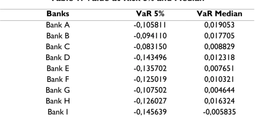
Estimated value-at-risk (VaR) of each bank using the coefficient generated from quantile regression of 5% and median VaR represents the tail probability of maximum loss of 5% and median. The estimation results of Value-at-Risk (VaR) on average during the critical condition (0.05 quantile) during the observation period showed that Bank I has the highest VaR value, which amounted to 14.56%, while the lowest VaR at Bank C, amounting 8.32%. The value of VaR at Bank I amounted to 14.56%. This means that there is a 5% possibility that investors will lose more than 14.56% of the portfolio value if investors choose Bank I as part of the portfolio. Interpretation from another point of view is the investor Bank I has a 95% chance that their losses will not exceed 14.56% of the portfolio. The value of VaR on Bank C of 8.32%. This means that there is a 5% possibility that investors will lose more than 8.32% of the value of the portfolio if investors choose Bank C as part of the portfolio. Interpretation from another point of view is the investor Bank C has a 95% chance that their losses will not exceed 8.32% of the portfolio.
Table 1. Value-at-Risk 5% and Median
Banks VaR 5% VaR Median
Bank A -0,105811 0,019053 Bank B -0,094110 0,017705 Bank C -0,083150 0,008829 Bank D -0,143496 0,012318 Bank E -0,135702 0,007651 Bank F -0,125019 0,010321 Bank G -0,107502 0,004644 Bank H -0,126027 0,016324 Bank I -0,145639 -0,005835
CoVaR measured using quantile regression coefficients obtained from Return on Assets System conditional on each return bank and economic factors (state variables). Estimation of Conditional Value-at-Risk (CoVaR) of each bank using the coefficient generated from quantile regression of 5% and 50% (median) represents CoVaR at 5% and median.Estimates of conditional value-at-risk (CoVaR) of each bank using the coefficient generated from quantile regression of 5% and a median representing CoVaR the tail probability of maximum loss of 5% and median.
Table 2. Conditional Value-at-Risk 5% and Median
Banks CoVaR 5% CoVaR Median
Bank A -0,067474 0,009361 Bank B -0,060764 0,012349 Bank C -0,051573 0,009991 Bank D -0,070341 0,013295 Bank E -0,053716 0,015109 Bank F -0,062614 0,014264 Bank G -0,054234 0,016360 Bank H -0,072669 0,013258 Bank I -0,050776 0,013417
The estimation results of Conditional Value-at-Risk (CoVaR) average at the time of critical conditions (quantile 0.05) during the observation period showed that Bank H has the highest CoVaR value, which amounted to 7.27%, while the lowest CoVaR on Bank I, ie by 5.08%.The value of the conditional VaR system, amounting to 7.27% when Bank H in a state of distress. That is the state of distress in Bank H will give effect to the system that impact the system will suffer a loss of 7.27%.The value of the conditional VaR system, amounting to 5.08% when Bank I in a state of distress. That is the state of distress in Bank I would give effect to the system that impact the system will suffer a loss of 5.08%.
Table 3. Marginal CoVaR (ΔCoVaR) Banks ΔCoVaR Bank A -0,076836 Bank B -0,073113 Bank C -0,061565 Bank D -0,083636 Bank E -0,068825 Bank F -0,076878 Bank G -0,070594 Bank H -0,085927 Bank I -0,064194
Marginal CoVaR (ΔCoVaR) represents the difference CoVaR at the time of distress and CoVaR condition when the condition of the median. The estimation results of marginal Conditional Value-at-Risk (ΔCoVaR) average over the study period showed that Bank H has the highest ΔCoVaR value, which amounted to 8.59%, while the lowest ΔCoVaR at Bank C, amounting to 6.16%.Value marginal CoVaR (ΔCoVaR) Bank H is 8.59% which means that PNBN contribute 8.59% of systemic risk in the system when migrating from the median VaR to the extreme, in this case VaR 5%. The value of the marginal CoVaR (ΔCoVaR) BBCA amounted to 6.16% which means that Bank C contribute 6.16% of systemic risk in the system when migrating from the median VaR to the extreme, in this case VaR 5%.
Testing individual correlation aims to determine whether there is a correlation between the value-at-risk (VaR) and marginal conditional value-at-risk (ΔCoVaR). Testing tools using Spearman correlation test and Kendall's Tau. The results of testing the correlation of each bank can be seen at Table 4. The correlation coefficient between VaR and ΔCoVaR calculated using Spearman correlation and correlation Kendall's Tau as has been shown in the research methodology. From the test results that the resulting correlation VaRand ΔCoVaR at Bank A, Bank E, Bank F, and Bank G showed no significant results. While the correlation of test results in Bank B, Bank C, Bank D, Bank H, and Bank I show significant results.
Table 4. Spearman and Kendall's Tau Correlation on Individual Bank
Banks Spearman Kendall’s Tau
Ρ Prob. τ Prob. Bank A 0,166838 0,0686 0,114566 0,0639 Bank B -0,369922 0,0000 -0,259664 0,0000 Bank C -0,206695 0,0235 -0,145938 0,0182 Bank D -0,658740 0,0000 -0,489356 0,0000 Bank E -0,001118 0,9903 0,003081 0,9620 Bank F 0,035877 0,6973 0,028011 0,6517 Bank G -0,040142 0,6633 -0,020168 0,7457 Bank H -0,265574 0,0034 -0,181513 0,0033 Bank I 0,479790 0,0000 0,340616 0,0000
The results of the calculations get that at Bank A, VaR has a positive correlation to ΔCoVaR. The magnitude of the correlation value against VaR to ΔCoVaR in Bank A can be seen from the value of ρ (rho) is 0.166838 and the value of τ (tau) is 0.114566. VaR of Bank E has a negative and positive correlation on ΔCoVaR with the value of ρ (rho) is -0.001118 and the value of τ (tau) is 0.003081. VaR of Bank F has a positive correlation on ΔCoVaR with the value of ρ (rho) is 0.035877 and the value of τ (tau) is 0.028011. And VaR of Bank G has a negative correlation onΔCoVaR with the value of ρ (rho) is -0.040142 and the value of τ (tau) is -0.020168.
In a scatter plot in Figure 1 shows the uneven distribution between individual risk (VaR) on the X axis and systemic risk contribution (ΔCoVaR) on the Y axis for each bank scatter plot shows a very weak relationship between VaR and ΔCoVaR. It can be concluded that to see the systemic risk contribution of each bank cannot rely solely on the size of VaR.
CONCLUSIONS
Results of research on systemic risk and ΔCoVaR shows VaR for each bank portion has a weak correlation and others do not have a significant correlation or in other words, almost no correlation. The results of the correlation calculations are under 0.50.At the end of 2008 the polemics in Indonesia when the Financial Stability Committee poured huge funds to save Bank Century. At that time the Bank Century was declared by the government as the bank failed to systemic risk. The complexity of defining the risk of systemic causes of this case became controversial.
The magnitude of the risk of individual banks does not mean proportional to the bank's contribution to systemic risk banks. In this study, Bank I has greater
individual risk among other banks, which amounted to 14.56%, while the contribution of the greatest systemic risk to the banking system is in Bank H, which amounted to 8.59%. Bank with value-at-risk (VaR) is high does not automatically become a bank which contribute greatly to the systemic risk in the banking system. So that needs to be done on the calculation method in addition to the value-at-risk (VaR) to assess the magnitude of systemic risk, one of them using a conditional value-at-risk (CoVaR).
In estimating the contribution of banks against systemic risk is not enough to look at the total assets of the bank. In this study, Bank H is a bank with the largest risk contribution (8.59%) had total assets eighth largest in Indonesia. In a state of crisis in the banking system, regulators would not only save the banks with total assets of large, but also the bank has total assets of small for the size is not the main reference for the contribution of banks to systemic risk. The failure of the banks that have small assets would trigger a rush to the bank to other banks the same level so that it can add to the uncertainty on the domestic market, which is fatal for the economy.
REFERENCES
Acharya, V.V., L.H. Pedersen, T. Philippon, & M. Richardson. (2010). Measuring Systemic Risk. Federal Reserve Bank Working Paper 10-02, March 2010.
Adrian, T. & M.K. Brunnermeier. (2011). CoVaR. National Bureau of Economic Research Working Paper,No. 17454, October 2011.
Arnold, B., C. Borio., L. Ellis, & F. Moshirian. (2012). Systemic Risk, Macroprudential Policy Frameworks, Monitoring Financial Systems and the Evolution of Capital Adequacy. Journal of Banking & Finance. 36: 3125-3132.
Ayomi, S. & B. Hermanto. (2013). Mengukur Risiko Sistemik dan Keterkaitan Finansial Perbankan di Indonesia (Measuring a Systemic Risk and Interlinkage of Financial Banking in Indonesia). Buletin Ekonomi Moneter dan Perbankan, 16 (2): 104-125. Benoit, S., G. Colletaz, C. Hurlin, & C. Périgon. (2013). A Theoretical and Empirical
Comparison of Systemic Risk Measures. HEC Paris Research Paper, No. FIN-2014-1030, June 2013.
Casu, B., C. Girardone, & P. Molyneux. (2006). Introduction to Banking. Essex: Pearson Education.
De-Bandt, O. & P. Hartmann. (2000). Systemic Risk: A Survey. European Central Bank Working Paper,No. 35, November 2000.
Dowd, K. & D. Blake. (2006). After VaR: The Theory, Estimation, and Insurance Applications of Quantile-Based Risk Measures. The Journal of Risk and Insurance. 73 (2): 193-229.
Drakos, A. A. & G. P. Kouretas. (2014). Measuring Systemic Risk in Emerging Markets Using CoVaR. In Emerging Markets and the Global Economy. M. Arouri, S. Boubaker, dan D. K. Nguyen (eds). Oxford: United Kingdom.
Gorton, G. (1988). Banking Panics and Business Cycles. Oxford Economic Papers. 40 (4): 751-781.
Gravelle, T. & F. Li. (2013). Measuring Systemic Importance of Financial Institutions: An Extreme Value Theory Approach. Journal of Banking & Finance. 37: 2196-2209. Huang, X., H. Zhou, & H. Zhu. (2009). A Framework for Assessing the Systemic Risk
of Major Financial Institutions”. Journal of Banking & Finance. 33: 2036–2049. Huang, X., H. Zhou, dan H. Zhu. (2011). Systemic Risk Contributions”. Journal of
Financial Services Research. 42 (1-2): 58-83.
Jorion, P. (2006). Value at Risk the New Benchmark for Managing Financial Risk. 3 ed. New York: The McGraw-Hill Companies.
Pais, A. & P. A. Stork. (2013). Bank Size and Systemic Risk. European Financial Management. 19 (3): 429-451.
Roengpitya, R. & P. Rungcharoenkitkul. 2011. “Measuring Systemic Risk and Financial Linkages in the Thai Banking System”. http://papers.ssrn.com/sol3/Delivery.cfm/ SSRN_ID1773208_code1243562.pdf?abstractid=1773208&mirid=1.
Segoviano, M. A. & C. Goodhart. (2009). Banking Stability Measures. International Monetary Fund Working Paper, WP/09/2, January 2009.
Wong, A. & T. Fong. (2010). Analysing Interconnectivity among Economies. Hong Kong Monetary Authority Working Paper 03/2010, May 2010.
Zhou, C. (2010). Are Banks Too Big to Fail? Measuring Systemic Importance of Financial Institutions. International Journal of Central Banking. 6 (4): 205-250.
Figure 1. Scatter Plot between VaR and ΔCoVaR each Banks -.14 -.12 -.10 -.08 -.06 -.04 -.02 -.5 -.4 -.3 -.2 -.1 .0 .1 .2 VaR 5% D e lt a C o V a R Bank A -.14 -.12 -.10 -.08 -.06 -.04 -.02 -.4 -.3 -.2 -.1 .0 .1 VaR 5% D e lt a C o V a R Bank B -.14 -.12 -.10 -.08 -.06 -.04 -.02 .00 -.4 -.3 -.2 -.1 .0 .1 VaR 5% D e lt a C o V a R Bank C -.16 -.14 -.12 -.10 -.08 -.06 -.04 -.6 -.5 -.4 -.3 -.2 -.1 .0 .1 VaR 5% D e lt a C o V a R Bank D -.12 -.10 -.08 -.06 -.04 -.02 -.5 -.4 -.3 -.2 -.1 .0 .1 VaR 5% D e lt a C o V a R Bank E -.14 -.12 -.10 -.08 -.06 -.04 -.02 -.4 -.3 -.2 -.1 .0 .1 VaR 5% D e lt a C o V a R Bank F -.12 -.10 -.08 -.06 -.04 -.02 -.5 -.4 -.3 -.2 -.1 .0 .1 VaR 5% D e lt a C o V a R Bank G -.18 -.16 -.14 -.12 -.10 -.08 -.06 -.04 -.02 .00 -.6 -.5 -.4 -.3 -.2 -.1 .0 .1 VaR 5% D e lt a C o V a R Bank H -.12 -.10 -.08 -.06 -.04 -.02 .00 -.4 -.3 -.2 -.1 .0 VaR 5% D e lt a C o V a R Bank I