Sufficient Dimension Reduction for Complex Data
Structures
A THESIS
SUBMITTED TO THE FACULTY OF THE GRADUATE SCHOOL OF THE UNIVERSITY OF MINNESOTA
BY
Shanshan Ding
IN PARTIAL FULFILLMENT OF THE REQUIREMENTS FOR THE DEGREE OF
Doctor of Philosophy
R. Dennis Cook, Advisor
c
Shanshan Ding 2014 ALL RIGHTS RESERVED
Acknowledgements
The years spent in graduate school at the University of Minnesota is one of the best time in my life. The journey of learning, studying, and doing research in Statistics has filled my life with enrichment, happiness, excitement and challenges. There are a number of people who have profound impact on my knowledge, ideas, and career goal, and to whom I am deeply indebted. Without them, my journey would not be so wonderful.
My deepest gratitude is extended to my advisor, Professor R. Dennis Cook. This thesis would not be accomplished without his tireless guidance, great inspiration, and tremendous support. He opened the door leading to academic research for me, and has continually inspired me with his scholarly wisdom and vision throughout the dissertation process. He has conveyed an innovative spirit in research and scholarship, a passion in teaching, and an earnest attitude in daily work. From him, I have seen a genius character, a scholar’s erudition, and a mentor’s noble personality and kind heart. These qualities have truly influenced me and made my life with vigor, dream, and positive energy. He is and will always be my role model.
My appreciation also goes to Professor Glen Meeden and Professor Christopher Nachtsheim for being my dissertation committee members and writing reference let-ters for my job application. I am thankful to Professor Birgit Grund who serves on my committee and provides insightful suggestions along the work. I am also grateful to Professor Tiefeng Jiang for his great advice and support in my job application and academic profession. I am indebted to Professor Galin Jones for enrolling me into the
agement during my graduate study, to Professor Adam Rothman for allowing me to audit his interesting lectures and sharing the lecture notes, and to Seth Mayottee for providing me with technical support on computer issues.
I would like to express my gratitude to all my friends and classmates who have helped me in one way or the other. Thank Dr. Xin Chen, Dr. Kofi Placid Adragni, and Dr. Zhihua Su for sharing their experiences and encouraging my grit in academic pursuit. Thank Dr. Liliana Forzani for her insightful discussion on dimension reduction problems. Thanks Dr. Qiqi Deng for her help with my internship application. Thank my officemates who brought me a lot of fun and made my PhD life more colorful. Thank my dear friends Joy Bai, Dr. Qian Li, Dr. Lu Xu, Shuling Li, Yalin Li, Junyan Shen, Dr. Shan Hu, Huimin Liu, Yingbo Hu, Sara Hosch, Nicholle Brokke, Dr. Chenxiao Da, Dr. Xingyuan Zeng, Jing Li, and many others for their great care and support.
The last but not the least, I would like to thank my parents for their fostering, and loving and caring me every time, every place, and in every way they can. My special thanks also go to my younger brother Deshi Ding, for sharing his ideas, values, and sense of humor with me, and to Wei Qian for all his love and support.
Dedication
To my mother Zhizhen Chen and my father Xiaochen Ding.
Abstract
Data with complex structures, such as array-valued predictors, or responses, are commonly encountered in modern statistical applications. Such data typically contain intrinsic relationship among the entries of each array-valued variable. Conventional sufficient dimension reduction (SDR) methods cannot efficiently utilize the data struc-tures and are inappropriate for the complex data. In this thesis, we propose a class of sufficient dimension reduction methods, including model-based dimension reduction methods: dimension folding principal component analysis (PCA) and dimension folding principal fitted components (PFC), moment-based sufficient dimension reduction meth-ods: tensor sliced inverse regression (SIR), and envelope methods to tackle data with array-valued predictors, or responses. The proposed methods can simultaneously re-duce a predictor’s, or a response’s, multiple dimensions without losing any information in prediction or classification. We study the asymptotic properties of these methods and demonstrate their efficiency in both theoretical and numerical studies.
Contents
Acknowledgements i Dedication iii Abstract iv List of Tables ix List of Figures xi 1 Introduction 1 1.1 SDR . . . 1 1.2 Outline . . . 3 1.3 Notations . . . 52 Dimension folding PCA and PFC 7 2.1 Dimension folding PCA . . . 9
2.1.1 Formulation of dimension folding PCA . . . 10
2.1.2 Estimation of dimension folding PCA . . . 12
2.1.3 Relationship with tensor PCA . . . 15
2.2 Dimension folding PFC . . . 16
2.2.1 Formulation of dimension folding PFC . . . 16
2.3 Robustness . . . 24
2.3.1 Misspecification of f(Y) . . . 24
2.3.2 Normality assumption . . . 25
2.4 Prediction . . . 27
2.5 Simulation studies . . . 29
2.5.1 Evaluation of estimation accuracy . . . 29
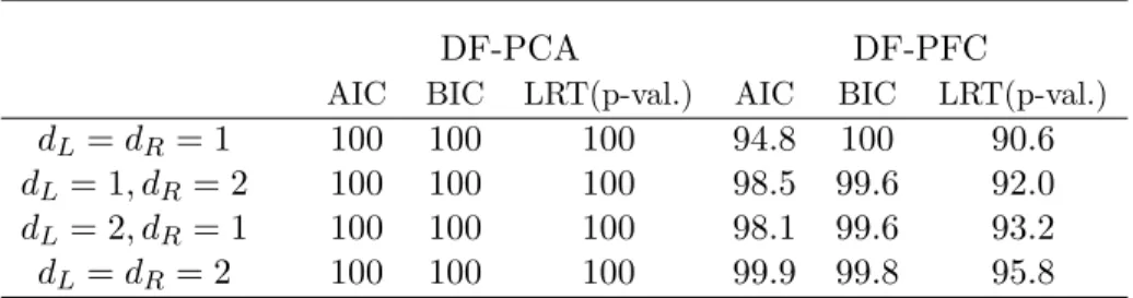
2.5.2 Choice ofdL anddR . . . 33
2.5.3 Prediction . . . 34
2.6 Data analysis . . . 35
2.6.1 EEG data . . . 36
2.6.2 Dow Jones stock data . . . 37
2.7 Discussion . . . 39
2.8 Appendix . . . 41
2.8.1 Matrix normal distribution . . . 41
2.8.2 Proofs . . . 42
3 Tensor sliced inverse regression 49 3.1 Motivation . . . 49
3.2 Two-tensor SIR . . . 51
3.2.1 A review of SIR . . . 51
3.2.2 Two-tensor SIR . . . 52
3.3 Multiple mode tensor SIR . . . 55
3.3.1 Methodology . . . 55
3.3.2 Kronecker tensor SIR . . . 59
3.4 Large sample properties . . . 60
3.5 Connections with other higher-order SDR methods . . . 63
3.5.1 Comparison of different linearity conditions . . . 63
3.5.3 Two-tensor SIR and longitudinal SIR . . . 65
3.5.4 Two-tensor SIR and dimension folding PFC . . . 66
3.6 Simulation studies . . . 67
3.6.1 Two-mode tensor predictors . . . 67
3.6.2 Three-mode tensor predictors . . . 69
3.7 Data analysis . . . 71
3.8 Discussion . . . 73
3.9 Appendix . . . 75
3.9.1 Proof of Lemma 3.1 and Lemma 3.2 . . . 75
3.9.2 Proof of Proposition 3.1 and 3.2 . . . 75
3.9.3 Proof of Lemma 3.3 and Lemma 3.4 . . . 76
3.9.4 Proof of Theorem 3.1 . . . 77
3.9.5 Proof of Theorem 3.2 . . . 80
3.9.6 Proof of Proposition 3.3 . . . 81
4 Matrix-variate regressions and the envelope models 83 4.1 Motivation . . . 83
4.2 Matrix-variate regression . . . 85
4.2.1 Model formulation . . . 85
4.2.2 Model estimation . . . 89
4.2.3 Goodness of fit . . . 91
4.3 Envelope models for matrix-variate regressions . . . 91
4.3.1 Introduction to envelopes . . . 91
4.3.2 Envelope formulation . . . 92
4.3.3 Maximum likelihood estimation . . . 95
4.3.4 Special cases . . . 97
4.4 Theoretical properties . . . 98
4.6 Simulation studies . . . 102
4.7 Applications . . . 105
4.7.1 Multivariate bioassay data . . . 105
4.7.2 EEG data . . . 111
4.8 Appendix . . . 113
4.8.1 Maximum likelihood estimation . . . 113
4.8.2 Proof of Lemma 4.1 . . . 115
4.8.3 Proof of Proposition 4.1 . . . 115
4.8.4 Proof of Propositions 4.2 and 4.3 . . . 116
4.8.5 Asymptotic properties of (4.22) . . . 117
4.8.6 Proof of Lemma 4.2 . . . 120
4.8.7 Proof of Proposition 4.4 . . . 120
4.8.8 Proof of Proposition 4.5 . . . 121
5 Future works 124 5.1 Semiparametric higher-order sufficient dimension reduction . . . 124
5.2 SDR for longitudinal data with ramdom effects . . . 125
References 127
List of Tables
2.1 Comparison of computation complexity . . . 23 2.2 Percentages of correct identifications . . . 34 2.3 Prediction results (×1000) with 10 folded cross validations . . . 38 3.1 Comparison of the CTS estimation among different higher-order SDR
methods for two-mode tensor predictors when a= 4. Each entry is the mean of the estimation errors (3.23) over 500 samples. . . 68 3.2 Comparison of the CTS estimation among different higher-order SDR
methods for two-mode tensor predictors whena= 50. Each entry is the mean of the estimation errors (3.23) over 500 samples. . . 69 3.3 Comparison of the CTS (or CS) estimation among different SDR methods
for three-mode tensor predictors whena= 4. Each entry is the mean of the estimation errors over 500 samples. . . 71 3.4 Comparison of the CTS (or CS) estimation among different SDR methods
for three-mode tensor predictors whena= 50. Each entry is the mean of the estimation errors over 500 samples. . . 72 4.1 Treatment assignment . . . 105 4.2 Comparison of the standard errors of vec( ˆα1) from the envelope and
stan-dard fits . . . 106 4.3 Comparison of the standard errors of vec( ˆβ) from the envelope and
stan-dard fits . . . 110
i
from the envelope and standard fits. . . 112
List of Figures
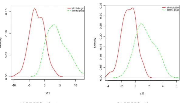
2.1 The comparison results of DF-PCA and PCA . . . 30 2.2 The comparison results of DF-PFC and PFC under general errors . . . 32 2.3 The comparison results of DF-PFC, DF-SIR and PFC . . . 33 2.4 Prediction results under isotropic errors . . . 35 2.5 Density plot with the new reduced predictorX11 . . . 37 3.1 Scatter plots by dimension reduced predictors X11, X12 with (sL, sR) =
(95,15). The triangles indicate alcoholic subjects. The circles represent nonalcoholic subjects. . . 74 4.1 The average estimation errors for the four group effects. The solid line indicates
the average estimation errors of the envelope models. The dashed line indicates the average estimation errors of the standard models. . . 103 4.2 The standard errors of the first elements in ˆαi obtained by the envelope model
and the standard model. The top three lines indicate the standard errors of the envelope models. The bottom three lines indicate the standard errors of the standard models. The solid lines marks the asymptotic standard errors; the thin dashed lines marks the bootstrap standard errors; and the heavy dashed lines marks the actual standard errors. . . 104 4.3 The SSPEs over differentu1 andu2. The solid line indicates the SSPE of
the standard model. The dashed line indicates the SSPEs of the envelope models for different choices ofu1 and u2. . . 107
1
line represents the SSPE of the standard matrix regression model. The dashed line represents the SSPEs of the envelope matrix regression models for different choices ofu1. . . 108 4.5 The SSPEs of the matrix regression models over differentu1. The solid
line represents the SSPE of the standard matrix regression model. The dashed line represents the SSPEs of the envelope matrix regression models for different choices ofu1. . . 110 4.6 The SSPEs over differentu1 andu2. The solid line indicates the SSPE of
the standard model. The dashed line indicates the SSPEs of the envelope models for different choices ofu1 and u2. . . 112
Chapter 1
Introduction
With the rapid development of data storage and computing technology, high dimensional data are frequently collected in a large variety of areas, such as biomedical engineering, neuroimaging, genomics, social media analysis, and high frequency finance. Dimension reduction is among major techniques in studying high dimensional data.
The basic idea of dimension reduction is to reduce the number of random variables in a dataset from a high dimensional space to a low dimensional space. Considerable dimension reduction methods have been studied in literature. For instance, principal component analysis (PCA) can be considered as one of the earliest and the most com-monly used dimension reduction methods in application. In addition, factor analysis, projection pursuit, independent component analysis, certain nonlinear dimension re-duction techniques such as principal curves and multidimensional scaling, and sufficient dimension reduction (SDR) approaches are also popular in practice.
1.1
SDR
In this thesis, we study dimension reduction methods mainly under the framework of sufficient dimension reduction. Sufficient dimension reduction is introduced by Cook (1994, 1998a). It is a paradigm of exploring dependency information through dimension
reduction. Let X ∈ Rp be a p-dimensional random predictor vector and Y ∈
R1 be
a response variable. Typical statistical problems study the relationship between Y and X in terms of the conditional distribution Y|X. When p is large, however, most statistical methods suffer the issue, so called the “curse of dimensionality”. Therefore, it is desirable to reduce the dimension of the predictor while preserving the full relationship between Y and X. Sufficient dimension reduction serves to achieve this goal. The key idea of SDR is to reduce the dimension of the predictor vector X by replacing it with its projection PSX onto a subspace S of the predictor space without loss of
information on the conditional distribution ofY|X. This requirement can be stated as Y X|PSX, where ‘ ’ indicates independence. Under mild conditions (Cook 1998a),
the intersection of all such dimension reduction subspaces S ⊆ Rp is also a dimension
reduction subspace and is called the central subspace, denoted as SY|X.
In some cases, one might not concern sufficient reduction for the full conditional distribution Y|X, but only for certain aspects of the dependency of Y on X. For instance, one might be only interested in the conditional mean of Y|X, denoted as E(Y|X). In this case, a dimension reduction subspace is defined as the subspaceS0 ⊆Rp
such that E(Y|X) = E(Y|PS0X). Again, the smallest dimension reduction subspace,
which is the intersection of all such dimension reduction subspaces, is of interest and it is called the central mean subspace (Cook and Li 2002), denotes asSE(Y|X). Depending on one’s specific need, the goal of SDR is to estimate SY|X, orSE(Y|X), or the smallest dimension reduction for the target of interest.
Research into sufficient dimension reduction has gained considerable momentum since early ’90s. Numerous dimension reduction methods can be incorporated into the rationale of sufficient dimension reduction under certain conditions. Sliced inverse regression (SIR; Li 1991) and sliced average variance estimation (SAVE; Cook and Weisberg 1991) are two early techniques for sufficient dimension reduction. Since then, principal Hessian directions (PHD; Li 1992, Cook 1998b), iterative Hessian transfor-mations (Cook and Li 2002), SDR for the conditional k-th moment (Yin and Cook
2002), SDR with categorical predictors (Chiaromonte et al. 2002), minimum average variance estimation (MAVE; Xia et al. 2002), bootstrap dimension reduction (Ye and Weiss 2003), inverse regression estimation (IRE; Cook and Ni 2005), directional regres-sion (DR; Li and Wang 2007), SDR for non-elliptical distributed predictors (Li and Dong 2009), semiparametric SDR (Ma and Zhu 2012), and many other methods were developed to either improve the estimation for SDR, or to perform SDR under different settings. While a few of the proposed methods employ nonparametric and semipara-metric techniques for estimation, most of them use the first two moments of X|Y for estimation, so called moment-based methods. In contrast, Cook (2007), and Cook and Forzani (2008, 2009) presented model-based SDR techniques, including principal fitted components (PFC), that give the maximum likelihood estimators (MLE) of the central subspace based on normal inverse models of X on Y. Model-based SDR inherits the optimal properties from maximum likelihood estimation and thus is more efficient than moment-based methods when the normality assumption holds. More recently, Cook et al. (2010, 2013) proposed a nascent research area, “Envelope models”, that combines the idea of SDR with multivariate analysis to achieve substantial gains in efficiency.
1.2
Outline
Although dimension reduction topics have been widely studied, the methods mainly fo-cus on a simple data structure: Y ∈R1andX ∈Rp. In modern statistical applications,
however, one often encounters more complex data structures, such as data with matrix-or array-valued predictmatrix-ors, matrix-or responses. In this thesis, we focus on such data and develop model-based SDR, moment-based SDR, and envelope models for array-valued data.
In Chapter 2, we propose model-based dimension folding methods mainly for data with matrix-valued predictors. The methods can be treated as extensions of conventional principal components analysis (PCA) and principal fitted components (PFC). We refer
to them as dimension folding PCA and dimension folding PFC. The proposed methods can simultaneously reduce a predictor’s multiple dimensions and inherit asymptotic properties from maximum likelihood estimation. They provide robust estimation and are computationally efficient. Dimension folding PFC gains further efficiency by effective use of the response information. Both theoretical and numerical results are provided to demonstrate the advantages.
In Chapter 3, we develop an efficient moment-based SDR method by extending SIR to general array (tensor)-valued predictors and refer to it as tensor SIR. Tensor SIR is constructed based on tensor decomposition to reduce an array-valued predictor’s multi-ple dimensions simultaneously. The proposed method provides fast and efficient estima-tion. It circumvents high-dimensional covariance matrix inversion that researchers often suffer when dealing with such data. We further investigate its asymptotic properties and show its advantages by simulation studies and a real data application.
Inspired by the idea of envelopes proposed by Cook et al. (2010), we establish matrix-variate regressions and their envelope models for data with matrix-valued predictors and responses in Chapter 4. The proposed methods can be naturally extended to array-valued regressions for array-array-valued predictors and responses. We study the estimation procedures and their asymptotic properties for the cases - with and without envelope structures. Under the envelope framework, immaterial information can be eliminated in estimation and the number of parameters can be notably reduced when the matrix-variate dimension is large. Therefore, the estimation can be much more accurate and efficient. We investigate these properties by both theoretical and numerical studies.
In chapter 5, we discuss some future works regarding SDR for complex data struc-tures.
1.3
Notations
To facilitate our discussion, the following notations are used in the thesis. The symbol U V|Z indicates the conditional independence of U and V given Z, and ∼ means identically distributed. For positive integers pand q,Rp×q denotes the class of all p×q
matrices. For A ∈Rp×q, span(A) denotes the subspace spanned by the columns of A,
PA = A(ATA)†AT denotes a projection operator onto span(A) relative to the usual
inner product, and QA = Ip −PA, where † is the Moore-Penrose inverse, and Ip is
the p ×p identity matrix. For a symmetric and positive definite matrix Σ ∈ Rp×p,
PA(Σ) = A(ATΣA)†ATΣ denotes a projection operator onto span(A) relative to the Σ-inner product. The Σ-inner product is defined as< X, X >=XTΣX forX ∈Rp.
For a subspace S ⊆ Rp and a square matrix B ∈
Rp×p, BS = {Bν : ν ∈ S}.
The symbol S⊥ stands for the orthogonal complement of S relative to the usual inner product. A basis matrix forS is any semi-orthogonal matrix whose columns form a basis for S. A matrixA∈Rp×q(q < p) is a semi-orthogonal matrix if ATA=Iq. When Ais
a basis matrix of S, we useA0 to denote a semi-orthogonal basis ofS⊥, where (A, A0) forms an orthogonal matrix. The notation G(u, r) stands for the Grassman manifold of dimension u inRr, which is a set of all u dimensional subspaces inRr.
For two square matricesB, C ∈Rp×p,Sd(B) denotes the span of the deigenvectors
of B corresponding to its d largest eigenvalues, and Sd(B, C) = B−12Sd(B− 1 2CB−
1 2).
When B ≥0,|B|0 indicates the product of non-zero eigenvalues of B. The notation ⊗ means the Kronecker product, and⊕denotes the direct sum of subspaces. For instance, the direct sum ofm subspacesV1,V2, . . . ,Vm is defined as
m
L
i=1
Vi={v1+v2+· · ·+vm :
v1 ∈ V1, v2 ∈ V2, . . . , vm ∈ Vm}. The symbol || · ||F stands for the Frobenius norm of a matrix or an array.
We use “vec” to indicate the vectorization operator that stacks the columns of a matrix into a vector, use “vech” to denote the half vectorization operator that stacks elements from the upper triangular or lower triangular part of a symmetric matrix into
Chapter 2
Dimension folding PCA and PFC
In modern statistical applications, data with matrix- or array-valued predictors, such as longitudinal data with p predictors observed over q times, EEG (electroencephalog-raphy) data, FMRI (functional Magnetic Resonance Imaging) data and general image data, are often encountered. The EEG data studied by Li et al. (2010) contains 122 subjects that are divided into alcoholic and control groups. For each subject, the pre-dictor contains measurements from 64 channels of electrodes placed on the subject’s scalp and sampled at 256 times. Thus the predictor is formed as a matrix of dimension 256×64, and the response is a binary variable indicating groups. The data structure can be represented as Y ∈ R1 and X ∈
RpL×pR. Traditional dimension reduction methods
are inadequate to analyze such complex data structures since they can only reduce the predictor’s dimension by vectorizing it, thus losing important information on its matrix structure.
In face recognition and image analysis, certain unsupervised dimension reduction techniques were developed to deal with such data, based only on the marginal distri-bution of X. These methods include 2DPCA (Yang et al. 2004), (2D)2PCA (Zhang
and Zhou 2005), GLRAM (Ye 2005), Unified PCA (Shan et al. 2008), probabilis-tic higher-order PCA (Yu, Bi and Ye 2011), etc. Li et al. (2010) proposed super-vised and moment-based dimension folding approaches that extend SIR, SAVE, and DR to data with matrix-valued predictors, in order to reduce the predictor’s row and column dimensions simultaneously without loss of information on Y|X. The idea of dimension folding can be expressed as the condition: Y⊥⊥X|ΓT
2XΓ1 or, equivalently,
Y⊥⊥vec(X)|(Γ1 ⊗Γ2)Tvec(X), where Γ1 ∈ RpR×dR and Γ2 ∈ RpL×dL have the
small-est column dimensions dR and dL (dR ≤ pR, dL ≤ pL). The subspace span(Γ1 ⊗Γ2) or, equivalently, span(Γ1) ⊗ span(Γ2) is called the central dimension folding (CDF) subspace for Y|X, and denoted as SY|◦X◦.
Like conventional moment-based methods, moment-based dimension folding ap-proaches are generally more efficient for discrete than for continuous responses, since their performance depends on how to slice the response variable in order to estimate the conditional mean or variance ofX|Y. The estimation can be inadequate if the num-ber of slices is not selected properly. Moreover, the moment-based dimension folding methods may not possess good asymptotic properties since they require inverting the high dimensional covariance matrix ˆΣ =dcov[vec(X)]. When the predictorX contains a large number of rows and columns, computational complexity and singularity issues in-trude. As a result, pre-screening is often necessary. To resolve these issues and improve efficiency, we propose model-based dimension folding methods, to be called dimension folding PCA and dimension folding PFC, that retain the key idea of dimension folding and obtain the MLE of the central dimension folding subspace. Dimension folding PFC gains further efficiency by effective use of the response information. The proposed meth-ods circumvent directly inverting ˆΣ and thus are more applicable to high dimensional data. In addition, dimension folding PCA and PFC provide robust estimators. They can be treated as generalized versions of conventional PCA and PFC since they include them as special cases.
dimension folding PCA and its estimation. Section 2.2 is devoted to the development of dimension folding PFC. Section 2.3 provides robustness results. Prediction methods are discussed in Section 2.4. Section 2.5 and 2.6 contain illustrations of the performance of our methods with simulation studies and data analysis. Discussion is given in Section 2.7. Technical details are given in Section 2.8.
2.1
Dimension folding PCA
Dimension folding PCA is a preliminary step to developing dimension folding PFC. It performs dimension reduction for data with matrix-valued predictors by reducing the predictor’s row and column dimensions simultaneously, so the predictor’s matrix information can be preserved. It is built on a normal inverse model of the predictor X ∈ RpL×pR on a latent matrix ν ∈ RdL×dR and provides the MLE of the central
dimension folding subspace.
Here is a brief review of conventional PCA methods. PCA was originally considered as a well-established data-analytic method not associated with any probabilistic model. Model-based PCA can be traced back to Tipping and Bishop (1999), where the PCA model was formulated as
X=µ+ Γν+σε. (2.1)
In their case, X ∈ Rp is the predictor vector, µ ∈
Rp is the overall mean of X, Γ ∈ Rp×d(d ≤ p) is a coefficient matrix with rank d, ν ∈ Rd is a latent random vector,
and ε∈Rp is the random error. Additionally, ν and ε are assumed to be independent
and both have standard multivariate normal distributions with zero means and identity covariance matrices. A random error with this structure is called an isotropic error. The identity covariance assumption for ν is not a restriction, since one can always combine a non-identity covariance matrix with Γ. Thus, the parameter Γ itself is not identified but span(Γ) is identified.
corresponds to the subspace spanned by the firstdeigenvectors of the sample covariance matrix ˆΣ ofX, which is the principal subspace obtained from data-analytic PCA. Cook (2007) proposed that when the latent variableν is replaced by some fixed, centered but unobserved values ν1, ..., νn, (2.1) can be considered as the regression of X on ν. Then
R(X) = ΓTX is a sufficient reduction satisfyingX|ΓTX, ν ∼X|ΓTX, where ‘∼’ stands
for equivalence. The MLE of span(Γ) is the same as the estimator obtained from (2.1) with the normal assumption for ν.
2.1.1 Formulation of dimension folding PCA
Dimension folding PCA incorporates the idea of dimension folding into the conventional PCA model (2.1). To achieve this, we assume that the matrix-valued predictor X is matrix normally distributed and has some intrinsic structure among its rows and columns to convey its matrix structure. The model is built on the inverse regression of the predictor as
X=µ+ Γ2νΓT1 +σε, (2.2) where X ∈ RpL×pR, Γ
1 ∈ RpR×dR (dR ≤ pR) and Γ2 ∈ RpL×dL (dL ≤ pL) are
semi-orthogonal matrices that reduce the column and row dimensions ofX,µ∈RpL×pR is the
overall mean ofX, andν∈RdL×dR is a latent matrix with mean zero. The random error
εis assumed to be independent ofνand have a matrix normal distribution. The matrix normal distribution is briefly reviewed in the appendix. As dimension folding PCA is a starting model, we simplify the error to be isotropic, so εis NpL×pR(0pL×pR, IpR, IpL).
More general error structures will be discussed in the dimension folding PFC section. In (2.2), neither Γ1 nor Γ2 is identified: if Γ1, Γ2 andν are replaced by Γ2A2, Γ1A1 and
A−21ν(AT1)−1, equation (2.2) remains the same, where A1 and A2 are any nonsingular matrices. Thus, the dimension folding PCA model depends on Γ1 and Γ2 only through their column spaces. Under (2.2),ν contains the coordinates of the centered conditional mean E(X|ν)−µrelative to Γ1 and Γ2, and the relationship E(X|ν)−µ=PΓ2[E(X|ν)−
µ]PΓ1 holds. Therefore, the predictor’s important row and column signals are preserved
by span(Γ1) and span(Γ2).
Model (2.2) reflects the homogeneous characteristic among the rows and columns of the centered conditional mean E(X|ν)−µ, because its column information is retained by the same Γ1 over all rows and its row information is preserved by Γ2 over all of its columns. This feature can be found in many data sets with matrix-valued predictors. For example, in the EEG data, the rows and columns of the predictors indicate the time and location measurements for each subject. It is reasonable to believe that the signals provided by the scalp locations are consistent over time, and vice versa. This is one major distinction between dimension folding PCA and conventional PCA, which omits the predictor’s intrinsic matrix information and simply converts it to a vector. In addi-tion to preserving the predictors’ matrix structure, another benefit of (2.2) is to greatly reduce number of parameters in estimation and improve accuracy. Meanwhile, when the column dimension of X is one, (2.2) is equivalent to the conventional PCA model (2.1) under the setting of Cook (2007). Thus, it is a generalization of the conventional model.
Model (2.2) can also be written in a vectorization version as
vec(X) = vec(µ) + (Γ1⊗Γ2)vec(ν) +σvec(ε). (2.3) Here vec(ε) has a multivariate normal distribution N(0pLpR, IpLpR). In this way,
di-mension folding PCA implies that under the isotropic error assumption, the centered conditional means E[vec(X|ν)]−vec(µ) fall in the subspace spanned by the columns of Γ1⊗Γ2.
A proposition connects the inverse regression models (2.2) and (2.3) to the dimension folding conditions.
Proposition 2.1. (a) Under (2.2), the distribution of ν|X is the same as the
distribu-tion of ν|ΓT
2XΓ1 over all values of X; (b) under (2.3), the distribution of ν|vec(X) is
Based on Proposition 2.1, R(X) = ΓT2XΓ1 is a sufficient reduction (folding) satis-fying X⊥⊥ν | Γ2TXΓ1. Since both Γ1 and Γ2 have the minimum column dimensions, span(Γ1⊗Γ2) forms the central dimension folding subspaceSν|◦X◦.
2.1.2 Estimation of dimension folding PCA
The parameters in (2.2) are estimated based on maximum likelihood. We assume that for each observation Xi of X, i = 1, ..., n, there is a corresponding coordinate matrix
νi, such that Xi = µ+ Γ2νiΓT1 +σε, where νi is fixed and n
P
i=1
νi = 0 without loss of
generality. In general, we are not able to find a closed-form solution for the MLE of the central dimension folding subspace. Yet we can apply a fast and stable algorithm that uses three eigen-based iterations and provides connections to the conventional PCA model.
For an independent sample{Xi}, according to (2.23), the full log likelihood of (2.2)
can be written as l(µ,SΓ1,SΓ2, σ 2, ν 1,· · ·, νn) =− npLpR 2 log(2π)− npLpR 2 logσ 2 − 1 2σ2 n X i=1 tr[(Xi−µ−Γ2νiΓT1)T(Xi−µ−Γ2νiΓT1)], (2.4) where SΓ1 and SΓ2 denote the column spaces span(Γ1) and span(Γ2). It is easy to see
that the MLE ˆµ = ¯X since
n
P
i=1
νi = 0. Then for any arbitrary σ2, maximizing (2.4) is
equivalent to minimizingPn
i=1tr[(Xi−X¯−Γ2νiΓT1)T(Xi−X¯−Γ2νiΓT1)], which can be solved based on the following.
Proposition 2.2. Suppose that Xi ∈ RpL×pR, i = 1, ..., n, are observed matrices. Let
(ˆΓ1,Γˆ2,νˆ1, ...,νˆn) be minimizers of n X i=1 tr[(Xi−G2ωiGT1)T(Xi−G2ωiGT1)] (2.5) over all G1 ∈RpR×dR, G 2 ∈RpL×dL, and ω i ∈RdL×dR, i= 1, ..., n. Then
(i) For fixedG1, the columns of the minimizerΓˆ2 are given by thedLeigenvectors of the
matrix ΣˆL=
n
P
i=1
XiP1XiT/n corresponding to its dL largest nonzero eigenvalues, where
P1=G1GT1.
(ii) For fixed G2, the columns of the minimizer Γˆ1 consist of the dR eigenvectors of the
matrix ΣˆR=
n
P
i=1
XiTP2Xi/n corresponding to its dR largest nonzero eigenvalues, where
P2=G2GT2.
(iii) For fixed G1 and G2, the minimizer ˆνi=GT2XiG1, i= 1, ..., n.
Based on Proposition 2.2, for fixed G1 and G2, ifωi is replaced by ˆνi =GT2XiG1, the objective function (2.5) is L1 = tr(
n P i=1 XiTXi)−tr[ n P i=1
(XiTP2Xi)P1]. Then for fixed P2, L1 is minimized by choosing the columns of G1 to be the firstdR eigenvectors of
n
P
i=1
XiTP2Xi. So we need to choose P2 to minimize L12 =
dR P k=1 λk( n P i=1 XiTP2Xi), where
λk(A) indicates thek-th eigenvalue ofA. This can be treated as an optimization problem
over a Grassmann manifold but it is hard to solve because eigenvalues are involved in the objective function. Instead, we apply an iterative algorithm that can solve the problem efficiently. We assume that the predictors are centered.
1. Generate an initial value of Γ10∈RpL×dL and let ˆΓ1 = Γ10. 2. For given ˆΓ1, compute the matrix ˆΣL=
Pn
i=1XiΓˆ1ΓˆT1XiT/n and find its firstdL
eigenvectors, denoted as ˆv1,ˆv2, ...,ˆvdL. Estimate Γ2 as ˆΓ2= [ˆv1,vˆ2, ...,ˆvdL].
3. For given ˆΓ2, compute ˆΣR=
Pn
i=1XiTΓˆ2ΓˆT2Xi/n; find the firstdReigenvectors of
ˆ
ΣR, denoted as ˆl1,ˆl2, ...,ˆldR, which form the columns of ˆΓ1 as ˆΓ1 = [ˆl1,ˆl2, ...,ˆldR].
4. For given ˆΓ1 and ˆΓ2, compute ˆνi= ˆΓT2XiΓˆ1,i= 1, ...., n.
5. Repeat Step 2 to 4 and iterate each time using the updated ˆΓ1 and ˆΓ2 until
Pn
i=1tr[(Xi−Γ2νiΓT1)T(Xi−Γ2νiΓT1)] converges.
The MLE of the central dimension folding subspaceSν|◦X◦is then equal to span(ˆΓ1)⊗ span(ˆΓ2). Consequently, ˆσ2is equal tonpL1pR Pni=1tr[(Xi−Γˆ2νˆiΓˆT1)T(Xi−Γˆ2νˆiΓˆT1)]. The
estimators obtained from the dimension folding model inherit the asymptotic properties of likelihood estimation under normality.
As with most optimization procedures, the proposed algorithm can convergence to a local minimum. It has a linear convergence rate. Our experience shows that the convergence behavior depends on the gaps between the eigenvalues of ˆΣL and the gaps
between the eigenvalues of ˆΣR. The larger the gaps, the more likely the algorithm
obtains a global solution. Meanwhile, according to our empirical study, the algorithm is quite stable with use of random initial values of Γ10. When a better initial value is required, one can choose the first dR eigenvectors of
Pn
i=1XiTXi/n as an initial Γ10,
where Pn
i=1XiTXi/n is the sample row covariance matrix of X.
The proposed estimation procedure has connections with conventional PCA and is easily interpreted. It can be seen that when the column reduction matrix Γ1 is known, the estimator of the row reduction Γ2 is the same as that of Γ in the conventional PCA model (2.1) with the original predictor Xi replaced by XiΓ1. Although here XiΓ1 is a matrix instead of a vector, the estimation logic remains the same. Similarly, if Γ2 is known, the column reduction Γ1 can be obtained from the conventional PC model with
Xi replaced by ΓT2Xi.
Compared to conventional PCA, dimension folding PCA is computationally efficient for dealing with matrix-valued predictors. The algorithm has three major steps at each iteration. An efficient way to compute ˆΣL is to perform multiplication for Xi and ˆΓ1 first and then multiply it by its transpose. Thus, the total computation cost of ˆΣL
is O(npLdR(pL+pR)). The eigen-decomposition of ˆΣL requires O(p2LdL) operations.
Similarly, it takesO(npRdL(pL+pR)) andO(p2RdR) operations to compute ˆΣR and its
eigenspace. The computation of ˆνi is of orderO(pLdR(pR+dL)). Therefore, dimension
folding PCA totally requires at mostO(max(pL, pR)2max(dL, dR)nm) operations, where
mis the number of iterations. Conventional PCA targeting vectorizedXcostsO(p2Lp2Rn) operations, which is more expensive under the mild condition that max(dL, dR)m <
2.1.3 Relationship with tensor PCA
Higher-order tensor decompositions have been widely studied in applied mathematics and engineering. Among them, the Tucker decomposition is considered as a higher order form of PCA, or tensor PCA (Kolda and Bader 2009). Here we discuss the connections of dimension folding PCA with tensor PCA. The key idea of tensor PCA is to decompose a tensor into a core tensor multiplied by a component matrix along each mode. Thus, in a two-mode tensor case whereX ∈RpL×pR, we haveX ≈GCHT, where
C ∈RdL×dR is the core matricized two-way tensor, andG ∈
RpL×dL and H ∈RpR×dR
are the component matrices. If dL and dR are less than pL and pR, the core tensor C
is considered as a compressed version of X. Thus, dimension reduction of the original tensor can be achieved. There are several ways to compute the Tucker decomposition. Major algorithms are developed to minimize the mean-squared loss function
f(G, H, C) =||X−Xˆ||F2 =||X−GCHT||2F. (2.6) This loss function has the equivalent form of the last term in our objective function (2.4). Kroonenberg and De Leeuw (1980) proposed an iterative least squares algorithm (ALS), called TUCKALS3 for computing a Tucker decomposition of three-way arrays. This method was further refined by De Lathauwer et al. (2000), where they enhanced the approximation by directly calculating the dominant subspaces rather than their individual singular vectors. From this aspect, the algorithm we presented for dimension folding PCA is equivalent to a sample version of the method in Lathauwer, Moor and Vandewalle (2000) for two-mode tensors.
Tensor PCA is a well-established data-analytic method but is not associated with any probabilistic model. Dimension folding PCA can be treated as a model-based ten-sor PCA. It gains properties from maximum likelihood estimation when the predictors are approximately normally distributed. The normality assumption, however, is not essential in our model and can be relaxed to a general distribution. In this case, dimen-sion folding PCA is equivalent to tensor PCA. The robustness of the dimendimen-sion folding
model regarding its normality assumption will be further discussed in Section 2.3.2.
2.2
Dimension folding PFC
Although dimension folding PCA can reduce the predictor’s row and column dimensions simultaneously, it performs dimension folding marginally and the relationship between the predictor and the response is omitted. Instead of regressing X on a latent matrix ν, dimension folding PFC models the inverse regression of X|Y and provides more informative estimation of the central dimension folding subspace SY|◦X◦.
2.2.1 Formulation of dimension folding PFC
The dimension folding PFC model can be formed in several ways depending on the relations between the predictors and response. One way is to fit the inverse regression by taking the true model to be
X=µ+ Γ2β2f(Y)β1TΓT1 +ε (2.7) or, equivalently,
vec(X) = vec(µ) + (Γ1⊗Γ2)(β1⊗β2)vec(f(Y)) + vec(ε), (2.8) wheref(Y)∈RrL×rR contains elements formalized as functions ofY,β
1 ∈RdR×rR(dR≤
rR) and β2 ∈ RdL×rL(d
L ≤ rL) are the coefficient matrices of rank dR and dL, and ε
is the random error independent of Y. It can be isotropic following the matrix normal distribution σNpL×pR(0pL×pR, IpR, IpL) or more general withNpL×pR(0pL×pR,Ω, M)
er-ror. In Section 2.3.2, we show that the normality assumption is not necessary in order to obtain consistent estimation. The other terms in (2.7) are defined as in Section 2.1.1. Based on (2.7), each coordinate Xij of X is a linear function of the elements in f(Y)
plus a random error. In addition, (ΓT2XΓ1)ij = (ΓT2µΓ1)ij+ rL X k=1 rR X l=1 β(2)ik β(1)lj f(Y)kl+ (ΓT2εΓ1)ij,
where βik(2) denotes the ik-th element ofβ2, βlj(1) denotes the lj-th element of β1T, and
f(Y)kl is thekl-th element off(Y),i= 1, ..., dL,j = 1, ..., dR. This shows a
multiplica-tive coefficient structure.
The functionf(Y) is determinable in some cases, for instance when inverse response plots (Cook 1998 (Chapter 10)) of Xij versus Y are informative about f(Y), or when
the response Y is categorical. In other cases, one can approximate f(Y) by a series of basis functions or piecewise basis functions. Usually f(Y) can be chosen as a diagonal matrix with dimensionrL=rR=r. We use this matrix form in the rest of this chapter.
When using polynomial approximations, f(Y) is then a diagonal matrix with diagonal elements ofY, Y2, ..., Yr. Correspondingly, the conditional expectation [ΓT2E(X|Y)Γ1]ij
is (ΓT2µΓ1)ij + r
P
k=1
βik(2)βkj(1)Yk, which often captures the main regression shape of X on Y when r is relative large. In fact, in Section 2.3.1 we show that in order to receive a consistent estimator for the central dimension folding subspace, the selected fitting function does not need to be very close to the true function, it is only required to be correlated to it. This indicates that an approximation with a finite dimension for f(Y) is generally adequate.
When the response Y is categorical, the fitting function f(Y) can be naturally determined. For instance, suppose that Y has h categories, then f(Y) can be simply chosen as a diagonal matrix of dimensionr =h−1 and itsk-th diagonal element can be specified as diag(f(Y))k=I(Y ∈Jk)−nk/n,k= 1, ..., h−1, whereJkindicates thek-th
category,nk is the number of observation inJk, andI(·) is the indicator function. The
sample solution of dimension folding PFC with a categorical response is not equivalent to that obtained by dimension folding SIR (Li et al. 2010). Dimension folding PFC is more efficient in estimation, does not involve computations relative to vec(X).
Compared with slicing-based methods, dimension folding PFC provides the flexi-bility to formulate the relationship between X and Y. It can more effectively use the response information by choosing an appropriate fitting function to perform dimension folding. Slicing function can be considered as one special choice for fitting f(Y) but
it is generally less accurate when Y is continuous. A proposition identifies the central dimension folding subspace for the dimension folding model (2.7).
Proposition 2.3. Under (2.7), when the random error ε is isotropic the central
di-mension folding subspace SY|◦X◦ = span(Γ1)⊗span(Γ2); when ε has a general
ma-trix normal distribution NpL×pR(0pL×pR,Ω, M), the central dimension folding subspace
SY|◦X◦=span(Ω−1Γ1)⊗span(M−1Γ2).
Other ways to formulate the dimension folding PFC model are discussed in Section 2.7. We focus on estimating model (2.7) with both isotropic error and general error in the next section. Without loss of generality, the predictor X and the fitting function f(Y) are assumed to be centered.
2.2.2 Estimation of dimension folding PFC Isotropic error
When εis isotropic with distribution σNpL×pR(0pL×pR, IpR, IpL), the central dimension
folding subspace SY|◦X◦ is equal to span(Γ1)⊗span(Γ2). For a random sample of size
n from (Y, X), the MLE of SY|◦X◦ is obtained based on the log likelihood function of
(2.7): l(µ,SΓ1,SΓ2, σ 2, β 1, β2) =− npLpR 2 log(2π)− npLpR 2 logσ 2− 1 2σ2× n X i=1 tr((Xi−µ−Γ2β2f(Yi)β1TΓT1)T(Xi−µ−Γ2β2f(Yi)β1TΓT1). (2.9)
It is easy to see that the MLE ˆµ= ¯X. Thus for any arbitraryσ2, maximizing (2.9) is equivalent to minimizing the empirical expectation
En{tr[(X−Γ2β2f(Y)β1TΓT1)T(X−Γ2β2f(Y)β1TΓT1)]} (2.10) over X and Y.
Proposition 2.4. Suppose that X ∈ RpL×pR is a random matrix and Y ∈
R1 is a
random variable. Let (ˆΓ1,Γˆ2,βˆ1,βˆ2) be minimizers of
En{tr[(X−G2b2f(Y)bT1GT1)T(X−G2b2f(Y)bT1GT1)]}. (2.11)
over all G1 ∈RpR×dR, G
2 ∈RpL×dL, b
1 ∈RdR×rR, and b
2∈RdL×rL. Then
(i) For fixed G1 and b1, the columns of the minimizer Γˆ2 over G2 are given by thedL
eigenvectors of the matrix
ΣfitL = En(XG1f
∗T
)[En(f∗f∗
T
)]−1En(f∗GT1XT)
corresponding to its dL largest nonzero eigenvalues, wheref∗ =f(Y)bT1. The minimizer
ˆ β2= ˆΓT2En(XG1f∗ T )[En(f∗f∗ T )]−1.
(ii) For fixed G2 and b2, the columns of the minimizer Γˆ1 over G1 consist of the dR
eigenvectors of the matrix
ΣfitR = En(X TG 2f∗)[En(f∗ T f∗)]−1En(f∗ T GT2X)
corresponding to itsdRlargest nonzero eigenvalues, where f∗ =b2f(Y). The minimizer
ˆ
β1= ˆΓT1En(XTG2f∗)[En(f∗
T
f∗)]−1.
Similar to Proposition 2.2, after replacing G2 and b2 with their optimum solutions ˆ
Γ2 and ˆβ2 obtained from Proposition 2.4(i), the problem becomes an optimization over a Grassmann manifold, but it is complicated to solve. Instead, we choose a simple iterative algorithm to estimate the likelihood function (2.9) as follows.
1. Generate initial values of Γ10 and β10 and let ˆΓ1 = Γ10 and ˆβ1 =β10. 2. For given ˆΓ1 and ˆβ1, compute the matrix ˆΣfitL = X
T
LPFLXL/n, where XL =
(X1Γˆ1, ..., XnΓˆ1)T, FL = (f1∗, ..., fn∗)T with fi∗ =f(Yi) ˆβ1T. Then the term PFLXL
represents the fitted values from the multivariate regression of XΓˆ1 on f(Y) ˆβ1T. Therefore, ˆΣfitL is the sample column covariance matrix of the fitted values of
XΓˆ1. Then the columns of ˆΓ2 are estimated by the first dL eigenvectors of ˆΣfitL
3. For given ˆΓ2 and ˆβ2, compute the matrix ˆΣfitR = X T RPFRXR/n, where XR = (X1TΓˆ2, ..., XnTΓˆ2)T, FR = (f∗ T 1 , ..., f∗ T
n )T with fi∗ = ˆβ2f(Yi). The term XTRPFR
represents the fitted values from the multivariate regression of ˆΓT2X on ˆβ2f(Y). Then ˆΣfitR represents the sample row covariance matrix of the fitted values of
ˆ
ΓT2X. The columns of ˆΓ1 are given by the first dR eigenvectors of ˆΣfitR and
ˆ
β1= ˆΓT1XTRFR(FTRFR)−1.
4. Repeat Steps 2-3 and iterate each time with the updated estimators until the objective function (2.10) converges.
The MLE of the central dimension folding subspace is then given by span(ˆΓ1)⊗span(ˆΓ2). Correspondingly,σ2 is estimated by 1 npLpR n X i=1 tr((Xi−Γˆ2βˆ2f(Yi) ˆβ1TΓˆT1)T(Xi−Γˆ2βˆ2f(Yi) ˆβ1TΓˆT1)).
It can be seen that the estimators ˆΓ1 and ˆΓ2obtained from dimension folding PFC have similar expressions as those achieved by dimension folding PCA. The only difference is that we perform eigen-decomposition for the sample row (column) covariance matrix of the fitted values of the linear regressions ˆΓT2X (XΓˆ1) on ˆβ2f(Y) (f(Y) ˆβ1T). In this way, the redundant information ofX that is not related toY is eliminated. Thus, dimension folding PFC is more precise in estimation and prediction. The estimators obtained from this algorithm can be treated as a generalized version of the results attained in conventional PFC.
From a computational perspective, the proposed algorithm is more economical than conventional PFC and dimension folding SIR. Its major costs come from the com-putation of ˆΣfitL and ˆΣfitR. For ˆΣfitL, computing XL and FL requires npLpRdR and
nrLrRdR operations, and computing XTLFL and FLTFL requires ndRpLrL and ndRr2L
operations. The inverse of FTLFL costs O(r3L). Therefore, the total cost of ˆΣfitL is
at most O(max(ndR, rL)max(pL, pR, rL, rR)2) . Similarly, the cost of ˆΣfitR is of order
error requires at most O(max(ndL, ndR, rL, rR)max(pL, pR, rL, rR)2m) operations with
m iterations. Analogously, it can be shown that the computations of conventional PFC and dimension folding SIR targeting on vec(X) take at leastO(max(n, pLpR)max(pLpR,
r)r) and O(p2Lp2Rmax(pLpR, n)k) operations, which are in general more than dimension
folding PFC when pL and pR are relative large. Here r is the dimension of the fitting
function in conventional PFC and kis the iteration number in dimension folding SIR. General error
In this section, we consider a general error structure for ε with the matrix normal distribution NpL×pR(0pL×pR,Ω, M). Based on this covariance structure, the dimension
folding models reveal another homogeneous characteristic among the predictor’s rows and columns. Let ei = (0, ...,0,1,0, ...0)T denote the pL-dimensional vector with ith
component equal to one, i = 1, ..., pL. Then eTi X = (vec(eTiX))T and var(eTi X|Y) =
var[(I⊗eTi )vec(X)|Y] = (I⊗eTi)(Ω⊗M)(I⊗ei) =miiΩ, where miiis theith diagonal
component ofM. This implies that the conditional covariance matrices of the predictor’s row vectors are all proportional to Ω. Similarly, the predictor’s column conditional covariance matrices are all proportional to M. Thus, the second-order moments also reflect the predictor’s intrinsic row and column structure, which the conventional PC and PFC models are not able to catch.
Another notable advantage is that the high-dimensional covariance matrix Σ = var[vec(X)] ∈ RpLpR×pLpR can be decomposed into two smaller matrices Ω ∈
RpR×pR
andM ∈RpL×pL. Therefore, one can circumvent inverting the sample covariance matrix
ˆ
Σ in estimation. This is beneficial when the sample size is relative small.
For estimation, note that if Ω andM are known, the problem reduces to the isotropic dimension folding PFC since one can standardizeXitoZi=M−
1 2XiΩ−
1
2. When Ω and
l(µ,SΓ1,SΓ2, β1, β2,Ω, M) =−npLpR 2 log(2π)− npL 2 log|Ω| − npR 2 log|M| −1 2 n X i=1 tr{Ω−1(X i−µ−Γ2β2f(Yi)β1TΓT1)TM−1(Xi−µ−Γ2β2f(Yi)β1TΓT1)}. (2.12) It is easy to see that the MLE of µ is ¯X. The other parameters can be es-timated by alternating iterations with one group of parameters fixed. Let XL =
(X1Ω− 1 2, ..., XnΩ− 1 2)T,FL= (f(Y1)βT 1ΓT1Ω− 1 2, ..., f(Yn)βT 1ΓT1Ω− 1 2)T, andXR= (XT 1M− 1 2, ..., XnTM−12)T,FR= (f(Y1)TβT 2ΓT2M −1 2, ..., f(Yn)TβT 2ΓT2M −1 2)T. Define ˆΣfit L =X T LPFL XL/npR, ˆMres = ˜M −ΣˆfitL =X T
LXL/npR−ΣˆfitL, and ˆΣfitR = X
T
RPFRXR/npL, ˆΩres =
˜
Ω−ΣˆfitR =X
T
RXR/npL−ΣˆfitR, where ˜Ω and ˜M are sample row and column covariance
matrices. Then the MLEs can be obtained based on the following.
Proposition 2.5. Suppose that Xi ∈ RpL×pR, i = 1, ..., n are observed and centered
matrices, and let (ˆΓ1,Γˆ2,βˆ1,βˆ2,Ωˆ,Mˆ) be the minimizers of (2.12).
(i) For fixedΩ,Γ1, andβ1, ifUˆLΛˆLUˆLT be the eigen-decomposition ofMˆ
−12
res ΣˆfitLMˆ
−12 res and ˆ
DLis the diagonal matrix with the firstdLeigenvalues ofΛˆLreplaced by zeros, thenMˆ =
ˆ Mres+ ˆM 1 2 resUˆLDˆLUˆLTMˆ 1 2 res, Γˆ2 = ˆM 1
2 times the first dL eigenvectors of Mˆ−
1 2Σˆfit LMˆ −1 2, and βˆ2 = ˆΓT2Mˆ−1XTLFL(FTLFL)−1.
(ii) For fixed M, Γ2, and β2, if UˆRΛˆRUˆRT is the eigen-decomposition of Ωˆ
−1 2 resΣˆfitRΩˆ −1 2 res
andDˆRis the diagonal matrix with the firstdReigenvalues ofΛˆRreplaced by zeros, then
ˆ Ω = ˆΩres+ ˆΩ 1 2 resUˆRDˆRUˆRTΩˆ 1 2 res,Γˆ1= ˆΩ 1
2 times the firstdR eigenvectors ofΩˆ−
1 2Σˆfit RΩˆ −1 2, and βˆ1 = ˆΓT1Ωˆ−1XTRFR(FTRFR)−1.
To estimate the parameters in (2.12), one can begin with initial estimates of Ω, Γ1, and β1, then iterate the two steps in Proposition 2.5 until the log likelihood function (2.12) converges. The computational cost of dimension folding PFC under a general
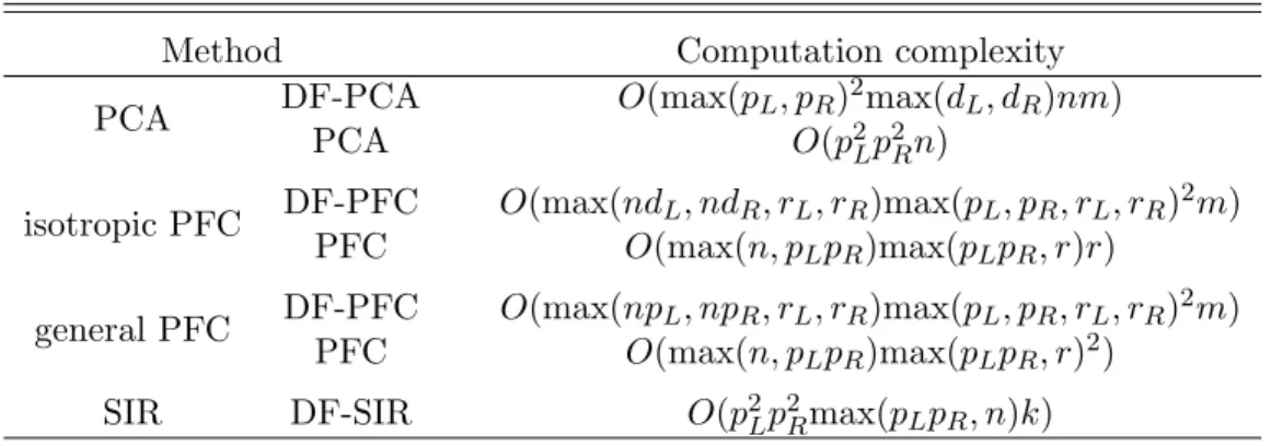
error is in general less expensive than that of conventional PFC and dimension folding SIR. We summarize the results for all models in Table 2.1.
Table 2.1: Comparison of computation complexity Method Computation complexity PCA DF-PCA O(max(pL, pR)
2max(d
L, dR)nm)
PCA O(p2Lp2Rn)
isotropic PFC DF-PFC O(max(ndL, ndR, rL, rR)max(pL, pR, rL, rR) 2m) PFC O(max(n, pLpR)max(pLpR, r)r)
general PFC DF-PFC O(max(npL, npR, rL, rR)max(pL, pR, rL, rR) 2m) PFC O(max(n, pLpR)max(pLpR, r)2)
SIR DF-SIR O(p2LpR2max(pLpR, n)k)
Remark 1. According to Proposition 2.5, ˆM is invertible when ˆMres is invertible. The existence of ˆMres−1 only requires that pL ≤ npR−1 and Rank(I −PFL) = pL. The
latter condition is generally satisfied since the nonzero eigenvalues of PFL are unlikely
to be exactly equal to one and they are unlikely to be all identical. Hence it is usually guaranteed that ˆM−1 and ˆΩ−1 exist ifpL≤npR−1 andpR≤npL−1 or, equivalently,
n >max(pL
pR,
pR
pL)−1.
Remark 2. The maximum matrix dimension required in Proposition 2.5 is npL×npL
ornpR×npR, from PFLor PFR. This dimension could be very large (>30000×30000) in
some cases (e.g. the EEG data) and exceed the storage limit in R software. In this case, one can apply an equivalent iteration algorithm that i) chooses moment estimators of Ω andM as initial values of ˆΩ and ˆM; ii) standardizes the predictors asZi = ˆM−
1 2XiΩˆ−
1 2;
iii) applies isotropic dimension folding PFC to the standardized data; iv) updates ˆΩ and ˆ
M according to (2.26) and (2.27), the MLEs of matrix normal distribution (Dutilleul 1999) described in the supplement file; v) repeats ii)-iv) using the updated parameter values until the likelihood function converges.
central dimension folding subspace based on random initial values, using the conven-tional PFC model to obtain initial values can guarantee consistency of the estimators when the fitted function f(Y) is misspecified. This is discussed in Sections 2.3 and 2.8. Corollary 2.1 provides five equivalent forms of the MLE of the central dimension folding subspace. We applied the original form SdR( ˆΩ,ΣˆfitR)⊗ SdL( ˆM ,ΣˆfitL) in our
simulation and data analysis.
Corollary 2.1. The MLE ofSY|◦X◦ under (2.7) with an general error isSdR( ˆΩ,ΣˆfitR)⊗
SdL( ˆM ,ΣˆfitL). It is equivalent to SdR( ˆΩres,ΣˆfitR)⊗ SdL( ˆMres,ΣˆfitL) = SdR( ˜Ω,ΣˆfitR)⊗
SdL( ˜M ,ΣˆfitL) =SdR( ˆΩ,Ω)˜ ⊗ SdL( ˆM ,M˜) =SdR( ˆΩres,Ω)˜ ⊗ SdL( ˆMres,M˜).
2.3
Robustness
In this section, we study the robustness of the estimator SdR( ˆΩ,ΣˆfitR)⊗ SdL( ˆM ,ΣˆfitL)
when f(Y) in model (2.7) is misspecified and the normality assumption is violated. 2.3.1 Misspecification of f(Y)
Under (2.7), we now assume that the true fitting functionf(Y) is misspecified by using the user-selected function h(Y) in place of f(Y). It can be shown that the estima-tor of the central dimension folding subspace is still consistent under certain condi-tions. To simplify the notation, let g = β2f(Y)β1T and l = κ2h(Y)κT1 be the mis-specified fitting components. Note that g and l are both centered. We take ρL =
var−
1 2
c (g)covc(g, l)var −12
c (l) to be thedL×dL column correlation matrix between the
el-ements ofg and l, where varc(g) = E(ggT) is the column variance of g, varc(l) = E(llT)
is the column variance of l, and covc(g, l) = E(glT) is the column covariance matrix
between g and l; let ρR = var −1
2
r (g)covr(g, l)var −1
2
r (l) be the dR×dR row correlation
matrix between the elements of g and l, where varr(g) = E(gTg) and varr(l) = E(lTl)
are row variance matrices of g and l, and covr(g, l) = E(gTl) is the row covariance
Proposition 2.6. SdR( ˆΩ,ΣˆfitR)⊗SdL( ˆM ,ΣˆfitL)is a
√
nconsistent estimator ofspan(Ω−1
Γ1)⊗span(M−1Γ2) if and only if ρL has rank dL and ρR has rank dR.
ThusSdR( ˆΩ,ΣˆfitR)⊗ SdL( ˆM ,ΣˆfitL) can still be a reasonable estimator whenf(Y) is
misspecified and the normality assumption is violated, as long as the row and columns correlations between the true fitting function and the selected fitting function have full ranks. This result is a generalization of Theorem 3.5 in Cook and Forzani (2008), and it is a mild condition. Nevertheless, in applications care should be taken when selecting f(Y) in order to obtain better estimates. Polynomial approximations can be simple and good choices.
2.3.2 Normality assumption
In applications, when the matrix-valued predictors do not satisfy the normality as-sumption, transformations such as log power are commonly used in literature (Gasser, B¨acher, and M¨ocks 1982) to achieve relative normality.
In addition, we show that the normality assumption is not essential for our model-based dimension folding methods. Suppose the random error εin model (2.2) follows a general distribution with mean zero and covariance matricesIPR andIPL. The unknown
parameters in this model can be estimated by minimizingPn
i=1||(Xi−µ−Γ2νiΓT1)||2F =
Pn
i=1tr[(Xi−µ−Γ2νiΓT1)T(Xi−µ−Γ2νiΓT1)]. Here the estimates span(ˆΓ1) and span(ˆΓ2) have the same expression as what we obtained under normality. Moreover, this objec-tive function is equivalent to the loss function (2.6) of the two-mode tensor PCA. The asymptotic normality and asymptotic efficiency of the projection matrix PΓˆ1⊗ˆΓ2 onto the estimated principal subspace span(ˆΓ1⊗Γˆ2) were developed by Hung et al. (2012). Hence without normality, one can still obtain√nconsistent estimators for the principal subspaces.
In terms of sufficient dimension reduction, the normality assumption can be re-laxed to the elliptically symmetric condition required by dimension folding SIR. Suppose vec(ε)∼ECpLpR(0,Ω⊗M, Q), where ECpLpR(0,Ω⊗M, Q) is an elliptical contoured
dis-tribution with mean zero, row and column covariance matrices Ω and M, and a density generator Q(.). Let ˜Y =sI(Y ∈Js), s= 1, ..., h, be the slice indicator function, where
J1, ..., Jharehnon-overlapping slices. Let ˜ζ = (Ω⊗M)−1E[vec(X)|Y˜], and letE⊗( ˜ζ) be
the Kronecker envelope of ˜ζ. According Li et al. (2010),E⊗( ˜ζ) is the dimension folding SIR subspace. It is defined as S◦ζ˜⊗ Sζ˜◦, the Kronecker product of the two smallest
subspaces S◦ζ˜ and Sζ˜◦, such that span( ˜ζ) ⊆ S◦ζ˜⊗ Sζ˜◦. The relationships between the dimension folding SIR subspace (Sf SIR), dimension folding PFC subspace (Sf P F C), and
central dimension folding subspace (SY|◦X◦) are shown below.
Proposition 2.7. Under (2.7), when the random error is elliptically contoured
dis-tributed asECpLpR(0,Ω⊗M, Q),Sf SIR⊆ Sf P F C ⊆ SY|◦X◦, whereSf P F C = span(Ω
−1Γ 1) ⊗span(M−1Γ2).
Thus, under the elliptically symmetric condition, the subspace span(Ω−1Γ1)⊗span(
M−1Γ2) given by dimension folding PFC is not guaranteed to be the true central di-mension folding subspace but a subspace of it. It contains the didi-mension folding SIR subspace at the population level and its sample estimate can be more accurate since the fitting function f(Y) is generally more efficient than a slicing function. Therefore, under this minimum condition, dimension folding PFC is still useful. Both algorithms in Section 2.2.2 provide√nconsistent estimators forSf P F C without normality, because
the algorithm for the isotropic error case in Section 2.2.2 is equivalent to a least square estimation and the consistent estimation of the algorithm for the general error case in Section 2.2.2 is given by Proposition 2.6, which does not rely on normality.
Similarly, Proposition 2.7 holds for dimension folding PCA in terms of Sν|◦X◦ and
ζ = E[vec(X)|ν]. Hence dimension folding PCA and PFC are beneficial under the minimum elliptically symmetric condition.
2.4
Prediction
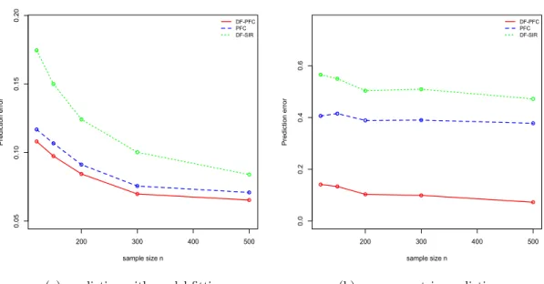
The ultimate purpose of dimension folding is to serve regression and classification. Di-mension folding SIR, SAVE, and DR proposed by Li et al. (2010) provide good pre-diction results in the classification case. Dimension folding PFC can further improve prediction accuracy for classification problems. In the regression case, where the re-sponse variable is continuous, the function of moment-based dimension folding methods is limited. Slicing could miss useful information on the response variable and the choice of slice number is a big issue. Dimension folding PFC can overcome this shortcoming and provide better prediction results.
We propose two prediction approaches. Based on our knowledge, there is no well-established method for predicting a univariate responses from a matrix-valued pre-dictor directly. Thus, we consider the prediction of Y from vec(X) instead. The first approach is to regress Y on vec(X) in two steps. By applying dimension fold-ing PCA or PFC, one can obtain the MLE of the central dimension foldfold-ing subspace
ˆ
SY|◦X◦ = span(ˆΓ1)⊗span(ˆΓ2) under an isotropic error, or ˆSY|◦X◦ = span( ˆΩ−1Γˆ1)⊗ span( ˆM−1Γˆ2) = SdR( ˆΩ,ΣˆfitR) ⊗ SdL( ˆM ,ΣˆfitL) under a general error. After
dimen-sion folding, one has a new predictor ˆΓT2XΓˆ1, or ˆΓT2Mˆ−1XΩˆ−1Γˆ1, with smaller row and column dimensions compared to the original predictor X. The second step is to fit a model, such as a general additive model (GAM), to estimate the mean function E[Y|vec(ˆΓT2XΓˆ1)] orE[Y|vec(ˆΓT2Mˆ−1XΩˆ−1Γˆ1)], and then perform prediction based on it.
The second method was motivated by a nonparametric prediction technique of Adragni and Cook (2009). Let f(X) and f(X|Y) be the density functions of X and X|Y. LetR(X) denote a sufficient folding assumed to have a density. Then E[Y|X = x] = E{Y f[R(x)|Y]}/E{f[R(x)|Y]}. This provides the key idea of this nonparamet-ric prediction approach because the estimated prediction function ˆE[Y|X =x] can be written as ˆE[Y|X =x] =Pn
i=1ωi(x)Yi, whereωi(x) = ˆf[ ˆR(x)|Yi]/
Pn
Once the density functionf(X|Y) is estimated, the predicted value ˆY can be easily obtained since it is the weighted average of the observed responses. This method is applicable to our proposed dimension folding models since the conditional distribution of X|Y is known through the model assumptions. According to (2.23) in Section 2.8, when the random errorε is isotropic we have
ˆ
f[ ˆR(x)|Yi] = ˆf[ ˆR(vec(x))|Yi]
∝exp{−(2ˆσ2)−1||(ˆΓ1⊗Γˆ2)T[vec(x)−vec( ˆXi)]||2}
= exp{−(2ˆσ2)−1||Rˆ(vec(x))−Rˆ(vec( ˆXi))||2},
(2.13)
where vec( ˆXi) = vec( ¯X)+(ˆΓ1⊗Γˆ2)( ˆβ1⊗βˆ2)vec(f(Yi)) is the predicted value of vec(x)|Yi
and the reduction ˆR(vec(x)) = (ˆΓ1 ⊗Γˆ2)Tvec(x). When ε has a general covariance structure, the estimated conditional density is
ˆ f[ ˆR(x)|Yi] = ˆf[ ˆR(vec(x))|Yi]∝exp{− 1 2||[(ˆΓ1⊗Γˆ2) T( ˆΩ⊗Mˆ)−1(ˆΓ 1⊗Γˆ2)]− 1 2 [ ˆR(vec(x))−Rˆ(vec( ˆXi))]||2}, (2.14)
where ˆR(vec(x)) = (ˆΓ1⊗Γˆ2)T( ˆΩ⊗Mˆ)−1vec(x).
Each method outperforms the other under certain conditions. The inverse regression prediction relies on the density function f[R(X)|Y] but does not make any parametric assumption on modeling Y|X, while forward regression prediction usually assumes a parametric model on Y|X or it depends on the estimation of Y|X. Thus, the inverse prediction method shows its advantages when the distribution of the random error ε in model (2.7) is known or can be well estimated. The forward prediction is beneficial when the assumption made on Y|X is reasonable.
In addition, the choice off(Y) can affect the prediction accuracy. Consider the mean squared error MSE = E[Y−Yˆ(X)]2for which the minimum prediction error is achieved when ˆY(X) is the conditional mean E(Y|X). According to Proposition 2.6, when the row and column correlations of the selected fitting function κ2h(Y)κ1 and the true function both have full ranks, which indicates that the two are correlated, the estimator
of the central dimension folding subspace is √n consistent. For the forward predic-tion method, we have ˆY(X) = ˆE(Y|Rˆ(X)) = ˆE(Y|ΓˆT2Mˆ−1XΩˆ−1Γˆ1). If one chooses
ˆ
E(Y|R(X)) to be a consistent estimator for E(Y|R(X)), such as the Nadaraya-Watson estimator, then under mild regularity conditions, ˆY(X)→E(Y|R(X)) = E(Y|X) when the selected fitting function is correlated to the true function. Thus the prediction error can reach its minimum asymptotically if the condition in Proposition 2.6 is satisfied. For the inverse prediction method, we have
ˆ E[Y|X =x] = 1 n n X i=1 ˆ f[ ˆR(x)|Yi]Yi , 1 n n X i=1 ˆ f[ ˆR(x)|Yi].
Assuming thatf(Y) is known, then it can be shown thatn1Pn
i=1fˆ[ ˆR(x)|Yi]→E{f[R(X)|Y]} and 1nPn
i=1fˆ[ ˆR(x)|Yi]Yi → E{Y f[R(X)|Y]} at
√
n rate. Then ˆE[Y|X = x] converges to E[Y|X =x] and the prediction error is asymptotically minimized. This result does not hold for misspecified f(Y) because the density function f[R(X)|Y] is misspecified in this case. Yet we can expect that the closer the approximation of the fitting function, the more likely we obtain good prediction.
2.5
Simulation studies
2.5.1 Evaluation of estimation accuracy
We assess the accuracy of our proposed dimension folding methods and compare it to that of conventional methods. We measure the difference between the estimated projection matrices and true projection matrices for the central dimension folding sub-space and denote it as “PCDF Error”; for conventional PCA and PFC, we evaluate the estimation error of the projection matrices of the central subspace and denote it as “PCS Error”. Specifically,
PCDF Error =kPSˆY|◦X◦−PSY|◦X◦k
2
PCS Error =kPSˆ
Y|vec(X)−PSY|◦X◦k
2
F. (2.16)
To evaluate the performance of the dimension folding PCA model (2.2), the data were generated as follows: LetdL=dR= 2 andpL=pR=p, with sample sizen= 100.
The components of Γ1and Γ2were generated fromN(0,1) and the componentsνibefore
centering were generated fromN(1,2),i= 1, ..., n. The vectorized isotropic errorεwas obtained from the multivariate normal with mean zero and covariance matrix 0.8IpLpR.
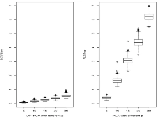
We chose p = 5,10,15,20 and 30, and ran each simulation 1000 times. The notations “DF-PCA”, “DF-PFC” and “DF-SIR” were used to denote dimension folding PCA, dimension folding PFC, and dimension folding SIR in figures and tables.
5 10 15 20 30 0 1 2 3 4 5 6 7
DF−PCA with different p
PCDF Error 5 10 15 20 30 0 1 2 3 4 5 6 7
PCA with different p
PCS Error
Figure 2.1: The comparison results of DF-PCA and PCA
noticeably more accurate than PCA. As the predictor’s dimension increases both meth-ods showed ascending estimation distance from the true projection space, but dimension folding PCA had the slower error increase in both the mean and standard deviation.
For dimension folding PFC, we did simulations for both isotropic and general error cases. When the general error structure was considered, we chose pL = pR = 3, dL =
dR= 2 and rL=rR= 4 . Conventional PFC and dimension folding SIR both required
n > pL×pR with a general error and we used small matrices pL×pR= 9 in this case.
The sample size was selected as n = 30,50,80,100 and 150. The components of Γ1 and Γ2 were generated from N(0,1). The elements of β1 and β2 were generated from
N(1,2) and absolute normal|N(2,2)|. The responsesYi,i= 1, ..., nwere obtained from
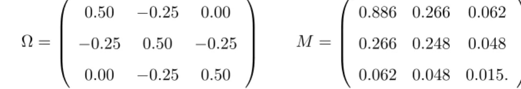
N(0,1), and f(Yi) = diag(Yi, Yi2, Yi3, Yi4). The covariance matrices were
Ω = 0.50 −0.25 0.00 −0.25 0.50 −0.25 0.00 −0.25 0.50 M = 0.886 0.266 0.062 0.266 0.248 0.048 0.062 0.048 0.015.
For the isotropic error case, we chose pL = pR = 10 and σ = 0.8, with sample size
n = 120,150,200,300,500. The other parameters were kept the same as those in the general error case. We ran the simulation 1000 times for each sample size.
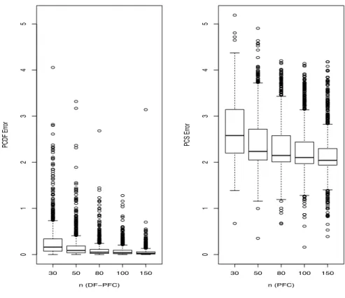
Figure 2.2 summarizes the results under the general error setting. It can be seen that the central dimension folding subspaces were estimated precisely based on the estimation procedures proposed in Section 2.2.2 except for some extreme outliers. Although the plots appear with dense outliers, the actual percentages of these outliers were less than 5% under 1000 repetitions. Some outliers like the one with estimation error close to 3 at n= 150 could be due to the algorithm getting caught in a local minimum. Conventional PFC had much higher estimation errors for all sample sizes.
30 50 80 100 150 012345 n (DFïPFC) PCDF Error 30 50 80 100 150 012345 n (PFC) PCS Error
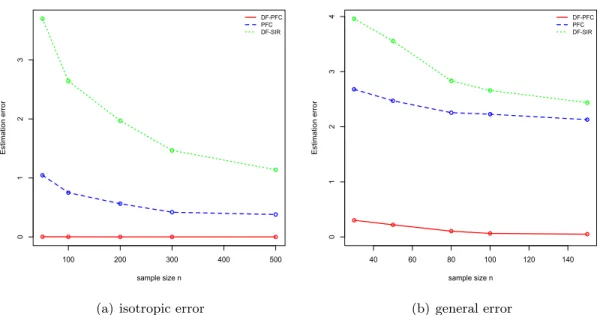
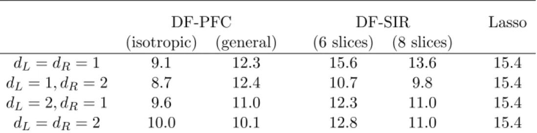
Figure 2.2: The comparison results of DF-PFC and PFC under general errors We further compared the model-based methods to dimension folding SIR. For the latter, 8 slices were selected for the response variable. Based on our simulation results, it was the best choice among 6, 8, 10 and 15 slices.
The mean estimation errors are shown in Figure 2.3, based on 1000 repetitions. It can be seen that dimension folding PFC provided the most accurate estimations for the central dimension folding subspace over all sample sizes. Although conventional PFC was less accurate than dimension folding PFC, it still beat dimension folding SIR to a large extent. Dimension folding SIR failed to obtain precise