Sparse Graphical Models
a dissertation
submitted to the faculty of the graduate school
of the university of minnesota
by
Lingzhou Xue
in partial fulfillment of the requirements
for the degree of
doctor of philosophy
Hui Zou, Adviser
First and foremost, I wish to take this opportunity to express my great appreciation to my advisor Professor Hui Zou. Over the last four years, I have been truly fortu-nate to have Professor Hui Zou as my advisor, mentor and friend. I am extremely grateful to Professor Hui Zou for influencing me with his enthusiasm, insights and professionalism, for supporting me with patience and encouragement in pursuing my interests and dreams, and for the numerous conversations about research, career and life. Thanks, Professor Hui Zou, for everything.
I am very grateful to Professor Charles Geyer, Professor Glen Meeden and Pro-fessor Fadil Santosa for serving on my thesis committee and providing me many insightful suggestions. My special thanks go to Professor Fadil Santosa for his en-couraging words and for generously introducing me to the Institute for Mathematics and its Applications and its 2012 Annual Program on Mathematics of Information.
I have been truly lucky to have met many excellent researchers and collaborators through my doctoral studies. I would like to thank Professor Runze Li, Professor Tianxi Cai, Professor Han Liu, Yu (David) Mao, Shiqian Ma, Teng Zhang and Qing Mai for their constant inspiration, stimulating discussions and close collaborations.
I wish to thank other faculty members in the School of Statistics for their support, availability and encouragement. I am thankful to all my friends for making my life at Minnesota a very enjoyable experience, and I will always cherish our friendship.
Last but not least, I want to thank my family for their love, support and encour-agement. I would like to dedicate this thesis to my parents and my girlfriend for their boundless love.
Dedicated to my parents Yiyu Xue, Yaohui Lin, and my girlfriend Qian Chen.
High-dimensional graphical models are important tools for characterizing complex interactions within a large-scale system. In this thesis, our emphasis is to utilize the increasingly popular regularization technique to learn sparse graphical models, and our focus is on two types of graphs: Ising model for binary data and nonpara-normal graphical model for continuous data. In the first part, we propose an effi-cient procedure for learning a sparse Ising model based on a non-concave penalized composite likelihood, which extends the methodology and theory of non-concave pe-nalized likelihood. An efficient solution path algorithm is devised by using a novel coordinate-minorization-ascent algorithm. Asymptotic oracle properties of our pro-posed estimator are established with NP-dimensionality. We demonstrate its finite sample performance via simulation studies and real applications to study the Human Immunodeficiency Virus type 1 protease structure. In the second part, we study the nonparanormal graphical model that is much more robust than the Gaussian graph-ical model while retains the good interpretability of the latter. In this thesis we show that the nonparanormal graphical model can be efficiently estimated by using a unified regularized rank estimation scheme which does not require estimating those unknown transformation functions in the nonparanormal graphical model. In partic-ular, we study the rank-based Graphical LASSO, the rank-based Dantzig selector and the rank-based CLIME. We establish their theoretical properties in the setting where the dimension is nearly exponentially large relative to the sample size. It is shown that the proposed rank-based estimators work as well as their oracle counterparts in both simulated and real data.
List of Tables vi
List of Figures vii
1 Introduction 1
2 Estimating Sparse Ising Models 4
2.1 Introduction . . . 4
2.2 Computing Algorithms . . . 8
2.2.1 The CMA algorithm . . . 9
2.2.2 Issues of local solution and the LLA-CMA algorithm . . . 11
2.3 Theoretical Properties . . . 15
2.4 Numerical Properties . . . 23
2.4.1 Monte-Carlo simulations . . . 23
2.4.2 Applications to the HIV drug resistance data . . . 27
3 Estimating Sparse Nonparanormal Graphical Models 31 3.1 Introduction . . . 31
3.2 Proposed Methodology . . . 37
3.2.1 The oracle procedures . . . 38
3.2.2 The proposed rank-based estimators . . . 41
3.2.3 Rank-based neighborhood LASSO? . . . 44
3.3 Theoretical Properties . . . 46
3.3.1 On the rank-based Graphical LASSO . . . 47
3.3.2 On the rank-based neighborhood Dantzig selector . . . 49
3.3.3 On the rank-based CLIME . . . 53
3.4 Numerical Properties . . . 56
3.4.1 Monte-Carlo simulations . . . 56
3.4.2 Applications to gene expression genomics . . . 62
4 Conclusion 64 4.1 Summary of Contributions . . . 64
4.2 Future Directions . . . 65
References 69 A Proof of Chapter 2 80 A.1 Proof of Theorem 2.1 . . . 81
A.2 Proof of Theorem 2.2 . . . 87
A.3 Proof of Corollary 2.1 . . . 93
A.4 Proof of Theorem 2.3 . . . 93
A.5 Proof of Corollary 2.2 . . . 95
B Proof of Chapter 3 96 B.1 Proof of Lemma 3.1 . . . 96 B.2 Proof of Theorem 3.1 . . . 99 B.3 Proof of Theorem 3.2 . . . 102 B.4 Proof of Theorem 3.3 . . . 106 B.5 Proof of Theorem 3.4 . . . 115 B.6 Proof of Theorem 3.5 . . . 116
2.1 Comparison of timing for different estimators in the simulation study. 25 2.2 Comparison of estimation/selection performance for different
estima-tors in the simulation study. . . 26 2.3 Comparison of selection performance for different estimators in the
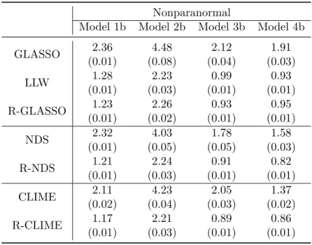
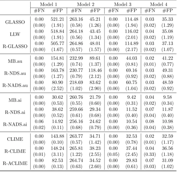
Stanford HIV drug resistance data. . . 28 3.1 Normality test for the isoprenoid gene expression data. . . 34 3.2 Summary of the sparsity in the simulated true precision matrices. . . 57 3.3 List of all estimators in the Monte Carlo simulation study. . . 58 3.4 Estimation performance in the Gaussian graphical model. . . 59 3.5 Estimation performance in the Nonparanormal graphical model. . . 59 3.6 Comparison of selection performance for different estimators in the
simulated normal data. . . 60 3.7 Comparison of selection performance for different estimators in the
simulated nonparanormal data. . . 61 3.8 Comparison of the bootstrap selection for different estimators in the
isoprenoid gene expression data. . . 62 4.1 Normality test for the small round blue-cell tumors microarray data. . 67 4.2 Normality test for the telephone call center data. . . 68
2.1 Plots of two synthetic Ising models in the simulation study. . . 25 2.2 Plots of stable edges for different estimators in the Stanford HIV drug
resistance data. . . 30 3.1 Illustration of the non-normality in the isoprenoid gene expression data. 34 4.1 Illustration of non-normality in the small round blue-cell tumors
mi-croarray data. . . 67 4.2 Illustration of non-normality in the telephone call center data. . . 68
Introduction
Nowadays, massive high-dimensional data are being routinely generated in various research fields, such as image processing, web mining, computational biology, climate studies, risk management and so on. How to succinctly characterizing complex inter-actions within a large-scale system is still an extremely challenging problem rooted in many real-world applications throughout science and engineering.
• One of our motivating examples is to study the associated viral mutations in the drug resistance of HIV-1-infected patients by investigating the inter-residue contacts between HIV-1 protease mutations and susceptibility to HIV antiretro-viral therapy drugs. The antiretro-viral mutation data are binary, and the Ising models from the statistical physics are usually used to study the underlying interactions of binary networks in practice. However, estimating the high-dimensional Ising model requires extremely intensive computation due to the intractable partition function. Thus, it is still a complicated task to discover the interaction patterns in the large scale binary network.
• The other motivating example is to analyze microarray gene expression measure-ments for recovering the isoprenoid genetic regulatory network in Arabidposis thaliana, which is one popular model organism in plant biology and genetics. The gene expression values are continuous data, and the common approach is
to study the underlying interactions (i.e. conditional dependencies) under the Gaussian graphical model. However, as evidenced in the normality test, the normal assumption usually appears to be inappropriate for the gene expression values with or without the log-transformation preprocessing. How to estimate the complex network effectively and efficiently from the high-dimensional non-normal data is still a difficult task.
In addition to these two examples, similar problems to construct large-scale binary or non-normal networks also arise in the real-world analysis of biological, geological, social or financial networks.
In this thesis, we emphasize the desirable parsimony in the estimation of graphical models, which offers an accurate predictive graph with a concise representation of complex interactions within a large-scale system. In particular, we utilize the well-developed regularization technique to learn sparse graphical models, and our focus is on two types of graphs: Ising model for binary data and nonparanormal graphical model for continuous data. In what follows, we outline the main results of this thesis. The details of Chapter 2 and Chapter 3 correspond to Xue et al. (2012) and Xue and Zou (2011) respectively.
In Chapter 2, we consider the problem of estimating a sparse Ising model for the binary data. To this end, we propose an efficient procedure for learning a sparse Ising model based on a non-concave penalized composite likelihood, which extends the methodology and theory of non-concave penalized likelihood. An efficient solution path algorithm is devised by using a novel coordinate-minorization-ascent algorithm. Asymptotic oracle properties of our proposed estimator are established with NP-dimensionality. Technical proofs are given in the Appendix A.
In Chapter 3, we consider the problem of estimating a sparse nonparanormal graphical model for the non-normal data. The nonparanormal graphical model is introduced as a robust alternative to the Gaussian graphical model, while it retains
the good interpretability of conditional independencies as in the latter model. We show that the nonparanormal graphical model can be efficiently estimated by using a unified regularized rank estimation scheme which does not require estimating these unknown transformation functions. In particular, we study the rate of convergence and the graphical model selection consistency of the rank-based Graphical LASSO, the rank-based Dantzig selector and the rank-based CLIME in the high-dimensional setting where the dimension is nearly exponentially large relative to the sample size. Simulated and real data demonstrate that the proposed rank-based estimators work as well as their oracle counterparts. Technical proofs are given in the Appendix B.
Estimating Sparse Ising Models
2.1
Introduction
The Ising model was first introduced in statistical physics (Ising, 1925) as a mathemat-ical model for describing magnetic interactions and the structures of ferromagnetic substances. Although rooted in physics, the Ising model has been successfully ex-ploited to simplify complex interactions for network exploration in various research fields such as social-economics (Stauffer, 2008), protein modeling (Irb¨ack et al., 1996), and statistical genetics (Majewski et al., 2001). Following the terminology in physics, consider an Ising model with K magnetic dipoles denoted by Xj, 1 ≤ j ≤ K. Each
Xj equals +1 or −1, corresponding to the up or down spin state of thej-th magnetic
dipole. The energy function is defined asE =−1 4(
P
i6=jβijXiXj), where the coupling
coefficientβij describes the physical interactions between dipolesXi andXj under the
external magnetic field,βii = 0 andβij =βji for any (i, j). According to Boltzmann’s
law, the joint distribution ofX = (X1,· · · , XK) should be
Pr(X1 =x1,· · · , XK =xK) = 1 Z(β)exp( X (i,j) βijxjxi 4 ), (2.1)
where Z(β) is the partition function.
In this chapter we focus on learning sparse Ising models, i.e., many coupling coefficients are zero. Our research is motivated by the HIV drug resistance study where understanding the inter-residue couplings (interactions) could potentially shed light on the mechanisms of drug resistance. A suitable statistical learning method is to fit a sparse Ising model to the binary data, in order to discover the inter-residue couplings. More details are given in Section 2.5. In the recent statistical literature penalized likelihood estimation has become a standard tool for sparse estimation. See a recent review paper by Fan and Lv (2010). In principle we can follow the penalized likelihood estimation paradigm to derive a sparse penalized estimator of the Ising model. Unfortunately, the penalized likelihood estimation method is very difficult to compute under the Ising model because the partition function Z(β) is computationally intractable when the number of dipoles is relatively large. On the other hand, the composite likelihood idea (Lindsay, 1988; Varin et al., 2011) offers a nice alternative. To elaborate, suppose we haveN independent identically distributed (iid) realizations ofX from the Ising model, denoted by{(x1n, ..., xKn), n= 1, ..., N}.
Let θj =P(Xi =xj|X(−j)), describing the conditional distribution of the jth dipole
given the remaining dipoles, whereX(−j) denotesX with thej-th element removed.
By (2.1), it is to easy see that for the n-th observation
θjn= exp(P k:k6=jβjkxjnxkn) exp(P k:k6=jβjkxjnxkn) + 1 .
Note thatθjndoes not involves the partition function. The conditional log-likelihood
of the j-th dipole given the remaining dipoles is given by
`(j) = 1 N N X n=1 log(θjn).
As in Lindsay (1988) a composite log-likelihood function can be defined as `c= K X j=1 `(j).
This kind of composite conditional likelihood was also called pseudo-likelihood in Besag (1974). Another popular type of composite likelihood is composite marginal likelihood (Varin, 2008). Maximum composite likelihood is especially useful when the full likelihood is intractable. Such an approach has important applications in many areas including spatial statistics, clustered and longitudinal data and time series models. A nice review on the recent developments in composite likelihood can be found in Varin et al. (2011).
To estimate a high-dimensional sparse Ising model, we consider the following penalized composite likelihood estimator
b β= arg max β {`c(β)− K X j=1 K X k=j+1 Pλ(|βjk|)} (2.2)
where Pλ(t) is a positive penalty function defined on [0,∞). In this work we focus
primarily on the LASSO penalty (Tibshirani, 1996) and Smoothly Clipped Absolute Deviation (SCAD) penalty (Fan and Li, 2001). The LASSO penalty is Pλ(t) = λt.
The SCAD penalty is defined by
Pλ0(t) =λ I(t≤λ) + (aλ−t)+ (a−1)λ I(t > λ) , t≥0; a >2.
Following Fan and Li (2001) we set a = 3.7. We should make it clear that when Pλ(t) is non-concave,βb should be understood as a good local maximizer of (2.2). See
discussions in Section 2.2.
(1) the number of unknown parameters is 12K(K −1) and hence the optimization problem is high-dimensional in nature; and (2) the penalty function is concave and non-differentiable at zero, although `c is a smooth concave function. We propose
to combine both strengthes of the coordinate-ascent and minorization-maximization principles, which results in two new algorithms, CMA and LLA-CMA, for computing a local solution of the non-concave penalized composite likelihood. See Section 2.2 for details. With the aid of the new algorithms, the SCAD penalized estimators are able to enjoy computational efficiency comparable to that of the LASSO penalized estimator.
Fan and Li (2001) advocated the oracle properties of the non-concave penalized likelihood estimator in the sense that it performs as well as the oracle estimator which is the hypothetical maximum likelihood estimator knowing the true submodel. Zhang (2010a) and Lv and Fan (2009) were among the first to study the concave penalized least-squares estimator with NP-dimensionality (i.e. pcan grow faster than any poly-nomial function of n). Fan and Lv (2011) studied the asymptotic properties of non-concave penalized likelihood for generalized linear models with NP-dimensionality. In this chapter we show that the oracle model selection theory remains to hold nicely for non-concave penalized composite likelihood methods with NP-dimensionality. Fur-thermore, we show that under certain regularity conditions the oracle estimator can be attained asymptotically via the LLA-CMA algorithm.
There is some related work in the literature. Ravikumar et al. (2010) viewed the Ising model as a binary Markov graph and used a neighborhood LASSO-penalized logistic regression algorithm to select the edges. Their idea is an extension of neigh-borhood selection by LASSO regression proposed by Meinshausen and B¨uhlmann (2006) for estimating Gaussian graphical models. H¨ofling and Tibshirani (2009) suggested using the LASSO-penalized pseudo-likelihood to estimate binary Markov graphs. However, they did not provide any theoretical result nor application. In this
chapter we compare the LASSO and the SCAD penalized composite likelihood esti-mators and show the latter has substantial advantages with respect to both numerical and theoretical properties.
The rest of this chapter is organized as follows. In Section 2.2, we introduce the CMA and LLA-CMA algorithms. The statistical theory is presented in Section 2.3. Monte Carlo simulation results are shown in Section 2.4. In Section 2.5 we present a real application of the proposed method to study the network structure of the amino-acid sequences of retroviral proteases using data from the Stanford HIV drug resistance database. Technical proofs are relegated to the Appendix A.
2.2
Computing Algorithms
In this section we discuss how to efficiently implement the penalized composite like-lihood estimators. As mentioned before, the computational challenges come from (1) penalizing the concave composite likelihood with a non-concave penalty which is not differentiable at zero; (2) the intrinsically high dimension of the unknown parame-ters. Zou and Li (2008) proposed the local linear approximation (LLA) algorithm to derive an iterative `1 optimization procedure for computing non-concave penalized
estimators. The basic idea behind LLA is the minorization-maximization principle (Lange et al., 2000; Hunter and Lange, 2004). Coordinate-ascent (or descent) algo-rithms (Tseng, 1988) have been successfully used for solving penalized estimators with LASSO-type penalties. See, e.g., Fu (1998), Daubechies et al. (2004), Genkin et al. (2007), Yuan and Lin (2006), Meier et al. (2008), Wu and Lange (2008) and Friedman et al. (2010). In this work we combine the strengthes of minorization-maximization and coordinatewise optimization to overcome the computational challenges.
2.2.1
The CMA algorithm
Letβe be the current estimate. The coordinate-ascent algorithm sequentially updates
˜
βij by solving the following univariate optimization problem
˜ βjk ⇐arg max βjk n `c(βjk;βj0k0 = ˜βj0k0,(j0, k0)6= (j, k))−Pλ(|βjk|) o . (2.3)
However, we do not have a closed-form solution for the maximizer of (2.3). The exact maximization has to be conducted by some numerical optimization routine, which may not be a good choice in the coordinate-ascent algorithm because the maximization routine needs to be repeated many times to reach convergence. On the other hand, one can find an update to increase rather than maximize the objective function in (2.3), maintaining the crucial ascent property of the coordinate-ascent algorithm. This idea is in line with the generalized E-M algorithm (Dempster et al., 1977) in which one seeks to increase the expected log likelihood in the M-step.
First, we observe that for any βij
∂2`c(β) ∂β2 jk =−1 N N X n=1 (θkn(1−θkn) +θjn(1−θjn))≥ − 1 2. (2.4)
Thus, by Taylor’s expansion we have
`c(βjk;βj0k0 = ˜βj0k0,(j0, k0)6= (j, k))≥Q(βjk) where Q(βjk) ≡ `c(βjk = ˜βjk;βj0k0 = ˜βj0k0,(j0, k0)6= (j, k)) +˜zjk(βjk −βejk)− 1 4(βjk − ˜ βjk)2 (2.5)
˜ zjk = ∂`c(β) ∂βjk β=βe = 1 N N X n=1 xknxjn(2−θkn(β)e −θjn(β)).e (2.6)
Next, Zou and Li (2008) showed that
Pλ(|βjk|)≤Pλ(|β˜jk|) +P
0
λ(|β˜jk|)·(|βjk| − |β˜jk|)≡L(|βjk|). (2.7)
Combining (2.5)–(2.7) we see thatQ(βjk)−L(|βjk|) is a minorization function of the
objective function in (2.3). We update ˜βjk by
˜
βjknew = arg max
βjk
{Q(βjk)−L(|βjk|)}, (2.8)
whose solution is given by
˜
βjknew =S( ˜βjk+ 2˜zjk,2Pλ0(|β˜jk|))
withS(r, t) = sgn(r)(|r|−t)+ being the soft-thresholding operator (Tibshirani, 1996).
The above arguments lead to the following Algorithm 1 which we call the coordinate-minorization-ascent (CMA) algorithm.
Algorithm 1 The CMA algorithm 1. Initialization of βe.
2. Cyclic coordinate-minorization-ascent: sequentially update ˜βij (1≤j < k ≤K)
via soft-thresholding ˜βjk ⇐S( ˜βjk+ 2˜zjk,2Pλ0(|β˜jk|)).
3. Repeat the above cycle till convergence.
Remark 3.1. It is easy to prove that Algorithm 1 has a nice ascent property which is a direct consequence of the minorization-maximizaton principle. Note that Algo-rithm 1 can be directly used to compute the LASSO-penalized composite likelihood
estimator. We simply modify the coordinate-wise updating formula as
˜
βjk ⇐S( ˜βjk+ 2˜zjk,2λ).
In practice we need to specify the λ value. BIC has been shown to perform very well for selecting the tuning parameter of the penalized likelihood estimator (Wang, Li and Tsai, 2007). The BIC score is defined as
ˆ λ= arg max λ {2`c(βb(λ))−log(n)· X (j,k) I( ˆβjk(λ)6= 0)}. (2.9)
The above BIC score is used to tune all methods considered in this work. We use SCAD1 to denote the SCAD solution computed by Algorithm 1 with the BIC tuned LASSO solution being the starting value.
For computational efficiency considerations, we implement Algorithm 1 by using the path-following idea and some other tricks including warm-starts and active-set-cycling (Friedman et al., 2010). We have implemented the algorithm in R language functions. The core cyclic coordinate-wise soft-thresholding operations were carried out in C.
2.2.2
Issues of local solution and the LLA-CMA algorithm
The objective function in (2.2) is generally non-concave if a non-concave penalty function is used. Using Algorithm 1 we find a local solution to (2.2) but there is no guarantee that it is the global solution. A similar case is Schelldorfer et al. (2011) where the objective function is the LASSO-penalized maximum likelihood of a high-dimensional linear mixed-effects model and the authors derived a coordinate-wise gradient descent algorithm to find a local solution.
Algo-rithm 1 or other coordinate-wise descent algoAlgo-rithm as in Schelldorfer et al. (2011) that the algorithm can only find a local solution, because in the current literature there is no algorithm that can guarantee to find the global solution of non-concave maximization (or non-convex minimization) problems, especially when the dimension is huge. Consider, for example, the E-M algorithm which is perhaps the most fa-mous algorithm in statistical literature. The E-M algorithm often offers an elegant way to fit some statistical models that are formulated as non-concave maximization problems. However, the E-M algorithm provides a local solution in general. A re-cent application of the E-M algorithm to high-dimensional modeling can be found in St¨adler et al. (2010) who considered a LASSO-penalized maximum likelihood estima-tor of a high-dimensional linear regression model with inhomogeneous errors that are modeled by a finite mixture of Gaussians. To handle the computational challenges in their problem, St¨adler et al. (2010) proposed a generalized E-M algorithm in which a coordinate descent loop is used in the M-step and showed that the obtained solution is a local solution.
Our numerical results show that in the penalized composite likelihood estimation problem the SCAD performs much better than the LASSO. To offer theoretical under-standing of their differences, it is important to show that the obtained local solution of the SCAD-penalized likelihood has better theoretical properties than the LASSO estimator. In Section 2.3 we establish the asymptotic properties of the LASSO es-timator and a local solution of (2.2) with the SCAD penalty. However, a general technical difficulty in non-concave maximization problems is to show that the com-puted local solution is the one local solution with proven theoretical properties. In St¨adler et al. (2010) and Schelldorfer et al. (2011), nice asymptotic properties are established for their proposed methods but it is not clear whether the computed local solutions could have those theoretical properties. The same issue exists in Fan and Lv (2011).
To circumvent the technical difficulty, we can consider combining the LLA idea (Zou and Li, 2008) and Algorithm 1 to solve (2.2) with a non-concave penalty. The LLA algorithm turns a non-concave penalization problem into a sequence of weighted LASSO penalization problems. Similar ideas of iterative LLA convex relaxation have been used in Candes et al. (2008), Zhang (2010b) and Bradic et al. (2011). Applying the LLA algorithm to (2.2), we need to iteratively solve
b β(m+1)= arg max β {`c(β)− K X j=1 K X k=j+1 wjk · |βjk|} (2.10) for m = 0,1,2, . . . where wjk = P 0 λ(|β˜ (m)
jk |). Note that Algorithm 1 can be used to
solve (2.10) by simply modifying the coordinate-wise updating formula as
˜
βjk ⇐S( ˜βjk+ 2˜zjk,2wjk).
Therefore, we have the following LLA-CMA algorithm for computing a local solution of (2.2).
Algorithm 2 The LLA-CMA algorithm 1. Initialize βe (0) and compute wjk =P 0 λ(|β˜ (0) jk |).
2. For m = 0,1,2,3, . . ., repeat the LLA iteration. (2.a) Use Algorithm 1 to solve βb
(m+1)
defined in (2.10). (2.b) Update the weights wjk byP
0
λ(|β˜
(m+1)
jk |).
In Section 2.3 we show that if the LASSO estimator is chosen as the initial solu-tion βe
(0)
then under certain regularity conditions the LLA-CMA algorithm finds the oracle estimator with an overwhelming probability, which is the maximum likelihood estimator over the true support set and will be formally introduced in Section 2.3.
In fact, after two LLA iterations, the LLA-CMA algorithm converges to the oracle estimator with probability tending to 1. These results suggest us to take the following steps to compute the SCAD solution by the LLA-CMA algorithm.
Proposed three-step procedure for computing a SCAD estimator
Step 1. Use Algorithm 1 to compute the LASSO solution path and find the LASSO estimator by BIC.
Step 2. Use the LLA-CMA algorithm to compute the two-step LLA-CMA solution path and find the two-step LLA-CMA solution by BIC.
Step 2a. Use the LASSO estimator as βe
(0)
in the LLA-CMA algorithm to compute the solution path. Choose the best λ by BIC and find the corresponding
e
β(1) as the one-step LLA-CMA estimator.
Step 2b. Use the one-step LLA-CMA estimator asβe
(0)
in the LLA-CMA algorithm to compute the solution path. Choose the best λ by BIC and the cor-responding βe
(1)
is referred as the two-step LLA-CMA solution in what follows and we denote it by SCAD2.
Step 3. For the chosen λ in Step 2b, use Algorithm 2 to compute the fully converged SCAD solution with SCAD2 being the starting value. Denote this SCAD solu-tion by SCAD2∗∗.
Note the fully converged LLA-CMA solution (i.e. SCAD2∗∗) is essentially com-puted by Algorithm 2 with the BIC tuned one-step LLA-CMA estimator being the starting value. Based on our experience, the fully converged SCAD2∗∗works slightly better than the two-step LLA-CMA solution (i.e. SCAD2) but these two solutions are generally very close. Both SCAD2 and SCAD2∗∗perform better than SCAD1, which is the solution by Algorithm 1. The tradeoff is that SCAD2 and SCAD2∗∗ require
almost another half computing time of that for SCAD1. Generally we recommend using SCAD2∗∗in the real-world applications. These numerical results are consistent with the numerical evidence provided by B¨uhlmann and Meier (2008) to advocate the two-step adaptive LASSO for the non-convex penalized regression problem.
2.3
Theoretical Properties
In this section we establish the statistical theory for the penalized composite con-ditional likelihood estimator using the SCAD and the LASSO penalty, respectively. Such results allow us to compare the SCAD and the LASSO estimators theoretically. In order to present the theory we need some necessary notation. For a matrix
A = (aij), we define the following matrix norms: the Frobenius norm kAkF =
q P
(i,j)a 2
ij, the entry-wise `∞ norm kAkmax= max(i,j)|aij| and the matrix`∞ norm
kAk∞ = maxi
P
j|aij|. Let β
∗
= {βjk∗ : j < k} denote the true coefficients. Define the true support set
A={(j, k) :βjk∗ 6= 0, j < k}
and its cardinality s = |A|. Define ρ(s, N) = min(j,k)∈A|βjk∗ | which represents the
weakness of the signal. Let H be the Hessian matrix of `c such that
H(j1k1),(j2k2) =−
∂2`c(β)
∂βj1k1∂βj2k2
for 1 ≤ j1 < k1 ≤ K and 1 ≤ j2 < k2 ≤ K. For simplicity we use H∗ = H(β∗).
We partition H and β according to A as
HAA HAAc HAcA HAcAc and β = (βTA,βTAc)T,
respectively. We let XA = (Xj : (j, k) or (k, j)∈ A for some k) and xAn= (xjn: (j, k) or (k, j)∈ A for some k). Finally, we define b=λmin(E[HAA∗ ]), B =λmax(E[XAXTA]) and φ=kE[HA∗cA](E[HAA∗ ])−1k∞.
Define the oracle estimator as
b βoracle = (βe hmle A ,0) where e
βhmleA = arg max
βA
`c((βA,0)).
If we knew the true submodel, then we would use the oracle estimator to estimate the Ising model.
Theorem 2.1 Consider the SCAD-penalized composite likelihood defined in (2.2). We have the following two conclusions.
(1) For any R < 3bB √ N s , we have Pr kβe hmle A −β ∗ Ak2 ≤ r s NR ≥1−τ1 (2.11) with τ1 = exp(−R2b 2 83) + 2s2exp(− N s2 b2 2) + 2s 2exp(−N s2 B2 8 ). (2) Pick a λ satisfying λ <min(ρ(s, N) 2a , (2φ+ 1)b2 3sB ).
With probability at least 1 −τ2, βb
oracle
is a local maximizer of the SCAD-penalized composite likelihood estimator where
τ2 = exp(−R2∗ b2 83) +K 2exp(− N λ2 32(2φ+ 1)2) + exp(− N λ 3B(2φ+ 1)s b2 83) +K 2sexp(−N b2 2s3 ) + 2s 2exp(−b2N 8s3 ) +4s2[exp(−N s2 b2 2) + exp(− N s2 B2 8 )] (2.12) and R∗ = min( 1 2 r N s ρ(s, N), b 3B √ N s ).
We also analyzed the theoretical properties of the LASSO estimator. If the LASSO can consistently select the true model, it must equal to the hypothetically oracle
LASSO estimator (βeA,0) where e βA = arg max βA {`c((βA,0))−λ X (j,k)∈A |βjk|}.
Theorem 2.2 Consider the LASSO-penalized composite likelihood estimator. (1) Choose λ such that λs < 83bB2, and then we have
Pr kβeA−β ∗ Ak2 ≤ 16λ√s b ≥1−τ10 with τ10 =e−N λ2/2 + 2s2[exp(−N b 2 2s2 ) + exp( −N B2 8s2 )].
(2) Assume the ir-representable condition that φ≤1−η <1. Choose λ such that
λs <min( b 2 162B η/3 4−η, 8b2 3B).
Then (βeA,0) is the LASSO-penalized composite likelihood estimator with
prob-ability at least 1−τ20, where
τ20 = e−N λ2/2+K2sexp(−N b 2η2 8s3 ) +K 2exp(− N λ2η2 32(4−η)2) +2s2[exp(− N b 2η2 2s3(2−η)2) + exp( −N b2 2s2 ) + exp( −N B2 8s2 )].
In Theorems 2.1 and 2.2 the three quantities b, B and φ do not need to be con-stants. We can obtain a more straightforward understanding of the properties of the penalized composite likelihood estimators by considering the asymptotic conse-quences of these probability bounds. To highlight the main point, we consider b, B
and φ are fixed constants and derive the following asymptotic results.
Corollary 2.1 Suppose that b,B and φ are fixed constants and further assume
N s3log(K) and ρ(s, N) r log(K) N .
(1) Pick the SCAD penalty parameterλscad satisfying
λscad<min(ρ(s, N) 2a , (2φ+ 1)b2 3sB ), λ scad r log(K) N .
With probability tending to 1, the oracle estimator is a local maximizer of the SCAD-penalized estimator and
kβb oracle A −β ∗ Ak2 =OP( r s N).
(2) Assume the ir-representable condition in Theorem 2.2. Pick the LASSO penalty parameter λlasso satisfying
min(√1 sρ(s, N), 1 s)λ lasso √1 N
then the LASSO estimator consistently selects the true model and
kβb lasso A −β ∗ Ak2 =OP(λlasso √ s).
Remark 3.2. For the LASSO-penalized least squares, it is now known that the model selection consistency critically depends on the ir-representable condition Meinshausen and B¨uhlmann (2006); Zou (2006); Zhao and Yu (2007). A similar condition is again needed in the LASSO-penalized composite likelihood. Furthermore, Corollary 2.1 shows that even when it is possible for the LASSO to achieve consistent selection, λlasso should be much greater than q1
N, which means that
λlasso√s
r
s N.
So the LASSO yields larger bias than the SCAD.
Remark 3.3. We have shown that asymptotically speaking the oracle estimator is in fact a local solution of the SCAD-penalized composite likelihood model. This property is stronger than the oracle properties defined in Fan and Li (2001). Our result is the first to show that the oracle model selection theory holds nicely for non-concave penalized composite conditional likelihood models with NP-dimensionality. The usual composite likelihood theory in the literature is only applied to the fixed-dimension setting. Our result fills a long-standing gap in the composite likelihood literature.
What we have shown so far is the existence of a SCAD-penalized estimator that is superior to the LASSO-penalized estimator. Moreover, we would like to show that the computed SCAD estimator is equal to the oracle estimator. As discussed earlier in Section 2.2, such a result is very difficult to prove due to the non-concavity of the penalized likelihood function. See also Fan and Lv (2011), St¨adler et al. (2010) and Schelldorfer et al. (2011).
If one can prove that the objective function has only one maximizer, then the computed solution and the theoretically proven solution must be the same. This idea has been used in Fan and Lv (2011) to study the non-concave penalized generalized
linear models and Bradic et al. (2012) to study the non-concave penalized Cox’s proportional hazards models. Their arguments are based on the observation that the SCAD penalty function has a finite maximum concavity (Zhang, 2010; Lv and Fan, 2009). Hence, if the smallest eigenvalue of the Hessian matrix of the negative log-likelihood is sufficiently large, the overall penalized likelihood function is concave and hence has a unique global maximizer. This argument requires the sample size is greater than the dimension, otherwise the Hessian matrix does not have full rank. To deal with the high-dimensional case, Fan and Lv (2011) further refined their arguments by considering a subspace denoted by Ss which is the union of all
s-dimensional coordinate subspaces. Under some regularity conditions, Fan and Lv (2011) showed that the oracle estimator is the unique global maximizer in Ss, which
was referred to as restricted global optimality. Then by assuming that the computed solution has exactly s nonzero elements, it can be concluded that the computed solution is in Ss and hence equals the oracle estimator. See Proposition 3.b of Fan
and Lv (2011). However, a fundamental problem with these arguments is that we have no idea whether the computed solution selects s nonzero coefficients, because s is unknown.
Here we take a different route to tackle the local solution issue. Instead of trying to prove the uniqueness of maximizer, we directly analyze the local solution by the LLA-CMA algorithm and discuss under which regularity conditions the LLA-CMA algorithm can actually find the oracle estimator.
Theorem 2.3 Consider the SCAD-penalized composite likelihood estimator in (2.2). Letβb
scad
be the local solution computed by Algorithm 2 (the LLA-CMA algorithm) with βe
(0)
being the initial value. Pick a regularization parameter λ satisfying
λ <min(ρ(s, N) 2a ,
(2φ+ 1)b2
Write τ0 = Pr(kβe
(0)
−β∗k∞> λ).
(1) The LLA-CMA algorithm finds the oracle estimator after one LLA iteration with probability at least 1−τ0 −τ3 where
τ3 = K2exp( −N λ2 32(2φ+ 1)2) + exp( −N λ 3B(2φ+ 1)s b2 83) +K 2 sexp(−N b 2 2s3 ) +2s2[exp(−N b 2 8s3 ) + exp(− N s2 b2 2) + exp(− N s2 B2 8 )].
(2) The LLA-CMA algorithm converges after two LLA iterations and βb
scad
equals the oracle estimator with probability at least 1−τ0−τ2, where τ2 is defined in
(2.12).
Theorem 2.3 can be used to drive the following asymptotic result.
Corollary 2.2 Suppose that b,B and φ are fixed constants and further assume
N s3log(K) and ρ(s, N) max( p log(K),16√s/b) √ N .
Consider the SCAD-penalized composite likelihood estimator with the SCAD penalty parameter λscad satisfying
λscad <min(ρ(s, N) 2a , (2φ+ 1)b2 3sB ), λ scad r log(K) N .
(1) If τ0 → 0, then with probability tending to one, the LLA-CMA algorithm
version) is equal to the oracle estimator. (2) Consider using the LASSO estimator as βe
(0)
. Assume the ir-representable con-dition in Theorem 2.2 and pick the LASSO penalty parameter λlasso satisfying
1 √ N λ lasso min(√1 sρ(s, N), 1 s), λ lasso< λ scad √ s b 16.
Then τ0 →0 and the conclusion in (1) holds.
Remark 3.4. Part (1) of Corollary 2.2 basically says that any estimator that con-verges toβ∗in probability at a rate faster thanλscadcan be used as the starting value in the LLA-CMA algorithm to find the oracle estimator with high probability. Note that such a condition is not very restrictive. Part (2) of Corollary 2.2 shows that the LASSO estimator satisfies that condition. We could also consider using other estima-tors as the starting value in the LLA-CMA algorithm. For example, we can use the neighborhood selection estimator as βe
(0)
. Following Ravikumar et al. (2010) we as-sume an ir-representable condition for each of theK neighborhood LASSO-penalized logistic regression and some other regularity conditions. Then it is not hard to show that the neighborhood selection estimator is also a qualified starting value. In this work, we would like to faithfully follow the composite likelihood idea and hence prefer to use the LASSO-penalized composite likelihood estimator as the starting value in the LLA-CMA algorithm.
2.4
Numerical Properties
2.4.1
Monte-Carlo simulations
In this section we use simulation to study the finite sample performance of the SCAD-penalized composite likelihood estimator. For comparison, we also include other two
methods: neighborhood selection by LASSO-penalized logistic regression (Ravikumar et al., 2010) and the LASSO-penalized composite likelihood estimator.
For each coupling coefficient βjk, the LASSO-penalized logistic method provides
two estimates: ˆβj7→k based on the model for the jth dipole and ˆβk7→j based on the
model for the kth dipole. Then we carry out two types of neighborhood selections: (i) aggregation by intersection (NSAI) based on ˆβNSAI
jk , and (ii) aggregation by union
(NSAU) based on ˆβNSAU
jk , where ˆ βNSAI jk = 0 if ˆβj7→kβˆk7→j = 0 ˆ βj7→k+ ˆβk7→j 2 otherwise and ˆ βNSAU jk = 0 if ˆβj7→k= 0 and ˆβk7→j = 0 ˆ βj7→k if ˆβj7→k6= 0 and ˆβk7→j = 0 ˆ βk7→j if ˆβj7→k= 0 and ˆβk7→j 6= 0 ˆ βj7→k+ ˆβk7→j 2 if ˆβj7→kβˆk7→j 6= 0 .
BIC has been shown to perform very well for selecting the tuning parameter of the penalized likelihood estimator (Wang et al., 2007; St¨adler et al., 2010; Schelldorfer et al., 2011). We used BIC to tune all competitors.
Two sparse Ising models were considered in our simulation. Their graphical struc-ture is displayed in Figure 1 where solid dots represent the dipoles and two dipoles are connected if and only if their coupling coefficient is non-zero. We generated the nonzero coupling coefficients as follows. If dipolesiandj are connected, we letβij be
tijsij where tij is a random variable following the uniform distribution on [1,2] and
(A) Model 1: 127 dipoles and 126 nonzero coupling coefficients.
(B) Model 2: 104 dipoles and 24 nonzero couplingcoefficients. Figure 2.1: Plots of two simulated Ising models.
we used Gibbs sampling to generate 100 independent datasets consisting 300 obser-vations. For comparison we use three measurements: the total number of discovered edges (NDE), the false discovery rate (FDR) and mean square errors (MSE).
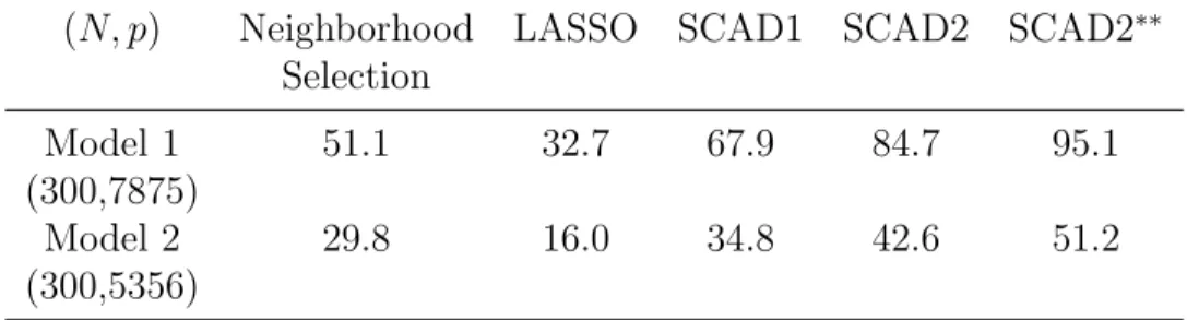
(N, p) Neighborhood LASSO SCAD1 SCAD2 SCAD2∗∗
Selection
Model 1 51.1 32.7 67.9 84.7 95.1
(300,7875)
Model 2 29.8 16.0 34.8 42.6 51.2
(300,5356)
Table 2.1: Total time (in seconds) for computing solutions at 100 penalization param-eters, averaged over 3 replications. Timing was carried out on a laptop with an Intel Core 1.60GHz processor. The timing of SCAD1, SCAD2 and SCAD2∗∗ includes the timing for computing the starting value.
In Table 2.1 we compare the run times of the three methods. Compared to the LASSO case, the run time for fitting the SCAD model is doubled or tripled, but it is still very manageable for the high-dimensional data.
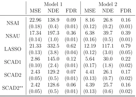
Based on the simulation results summarized in Table 2.2, we make the following interesting observations:
Model 1 Model 2
MSE NDE FDR MSE NDE FDR
NSAI 22.96 138.9 0.09 8.16 26.8 0.16 (0.18) (0.4) (0.01) (0.12) (0.2) (0.01) NSAU 17.34 197.3 0.36 6.38 39.7 0.39 (0.14) (1.0) (0.01) (0.16) (0.5) (0.01) LASSO 21.33 332.5 0.62 12.19 117.1 0.79 (0.13) (3.8) (0.04) (0.12) (3.0) (0.05) SCAD1 2.86 145.0 0.12 5.64 30.0 0.22 (0.10) (2.4) (0.01) (0.17) (1.8) (0.02) SCAD2 2.43 129.2 0.07 4.41 26.1 0.17 (0.05) (0.5) (0.01) (0.13) (0.7) (0.02) SCAD2∗∗ 2.42 128.6 0.06 4.39 25.7 0.16 (0.05) (0.5) (0.01) (0.13) (0.6) (0.02)
Table 2.2: Comparing different estimators using simulation models 1 and 2 with standard errors in the bracket.
• NSAU, while selecting larger models than NSAI, provides more accurate esti-mation. Neighborhood selection outperforms the LASSO-penalized composite likelihood estimator.
• Note that SCAD2∗∗ has the smallest MSE in both models. SCAD2∗∗ and SCAD2 gave almost identical results and their improvement over SCAD1 is statistically significant. All three SCAD solutions perform much better than the LASSO for fitting penalized composite likelihood in terms of estimation and selection.
• The SCAD solutions and NSAI have similar model selection performance, but the SCAD is substantial better in estimation. Using the relaxed LASSO can improve the estimation accuracy of neighborhood selection methods, but their improved MSEs are still significantly higher than those of SCAD2 and SCAD2∗∗.
2.4.2
Applications to the HIV drug resistance data
We illustrate our methods in a real example using a HIV antiretroviral therapy (ART) susceptibility dataset obtained from the Stanford HIV Drug Resistance Database (Rhee et al., 2004). The data for analysis consists of virus mutation information at 99 protease residues forN = 702 isolates from the plasma of HIV-1-infected patients. This dataset has been previously used in Rhee et al. (2006) and Wu et al. (2010).
A well recognized problem with current ART treatment such as PIs for treating HIV is that individuals who initially respond to therapy may develop resistance to it due to viral mutations. HIV-1 protease plays a key role in the late stage of viral replication and its ability to rapidly acquire a variety of mutations in response to various PIs confers the enzyme with high resistance to ARTs. A high cooperativity has been observed among drug-resistant mutations in HIV-1 protease (Ohtaka et al., 2003). The sequence data retrieved from treated patients is likely to include mutations that reflect cooperative effects originating from late functional constraints, rather than stochastic evolutionary noise (Atchley et al., 2000). However, the molecular mechanisms of drug resistance is yet to be elucidated. It is thus of great interest to study inter-residue couplings which might be relevant to protein structure or function and thus could potentially shed light on the mechanisms of drug resistance. We apply the proposed method to the protease sequence data to investigate such inter-residue contacts. Our analysis included K = 79 of the 99 residues that contain mutations.
We split the data into a training set with 500 data and a test set with 202 data. Model fitting and selection were done on the training set and the test data were used to compare the model errors. For a given estimate βb obtained from the training set,
its model error is gauged by the composite likelihood evaluated on the test set, i.e.,
ME(βb) = −`testc (βb) =− 1 202 202 X n=1 79 X j=1 log(θjn(βb)).
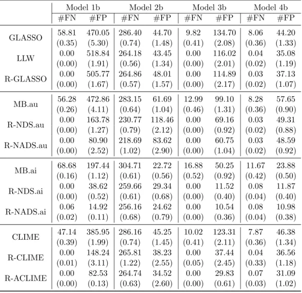
NSAI NSAU LASSO SCAD1 SCAD2 SCAD2∗∗
NDE 57 305 631 101 141 132
ME 26.38 36.34 18.35 18.30 16.76 16.74
Stability selection NSAI NSAU LASSO SCAD1 SCAD 2 SCAD2∗∗
NSE (πthr= 0.9) 15 63 160 17 20 20
E[V] ≤3.2 ≤48 ≤147.5 ≤4.3 ≤8.0 ≤7.2
Table 2.3: Application to HIVRT data. NSE is the number of “stable edges”. E[V] is the expected number of falsely selected edges. Its upper bounds were computed by Theorem 1 in Meinshausen and B¨uhlmann (2009).
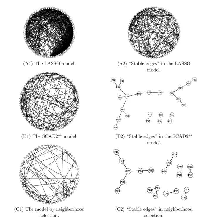
We report the analysis results in Table 2.3. There are total 3081 coupling coeffi-cients to be estimated. Graphical presentations of the selected models are shown in Figure 3.2. Note that SCAD2 and SCAD2∗∗ again gave almost identical results and performed better SCAD1. We also performed stability selection (Meinshausen and B¨uhlmann, 2010) on each method to find “stable edges”. A remarkable property of stability selection is that under some suitable conditions stability selection achieves finite sample control over the expected number of false discoveries in the set of “sta-ble edges”. We use the SCAD selector to explain the stability selection procedure. We took a random subsample of size 250 and fitted the SCAD model. The process was repeated 100 times. On average, SCAD1 selected 103.1 edges, SCAD2 selected 140.7 edges and SCAD2∗∗ chose 133.4 edges. For each coefficient βjk we computed
its frequency of being selected, denoted by ˆΠjk. The set of “stable edges” is
de-fined as {(k, j) : ˆΠkj > πthr}. In Table 3, we report the results using the threshold
πthr = 0.9, as suggested by Meinshausen and B¨uhlmann (2009). Stability selection
found 17 edges in the SCAD1. SCAD2 and SCAD2∗∗ selected the same 20 stable edges. By theorem 1 in Meinshausen and B¨uhlmann (2009), among these 17 stable edges selected by SCAD1, the expected number of false discoveries is no greater than 4.3, and among the 20 stable edges selected by SCAD2 or SCAD2∗∗, the expected
number of false discoveries is at most 7.2. Likewise, we did stability selection with the LASSO selector and neighborhood selection and the results are reported in Table 3 as well. Figure 3 shows the “stable edges” by stability selection. We see that the computed upper bounds are very useful for the SCAD selector and NSAI and not so informative for the LASSO selector and NSAU. Interestingly, both NSAI and SCAD suggest there are about 12 true discoveries by stability selection. In fact, we found that NSAI and SCAD have 11 “stable edges” in common, and NSAI and SCAD2 (or SCAD2∗∗) have 12 “stable edges” in common.
These results are consistent with some of the previous findings. For example, it has long been known that co-substitutions at residues 30 and 88 are most effective in reducing the susceptibility of nelfinavir (Liu et al., 2008). Among the top 30 most common drug resistance mutations (Rhee et al, 2004), 7 of those had a joint mutation at residues 54 and 82, the joint mutation at residues 88 and 30 was the second most common mutations among all. A co-mutation at residues 54, 82 and 90 was associated with high resistance to multiple drugs and an additional co-mutation at 46 was associated with an even higher level of resistance. It is interesting to note that using a larger set of isolates from treated HIV patients, Wu et al. (2003) reported (54, 82), (32, 47), (73, 90) as the three most highly correlated pairs. All these three pairs showed up as the stable edges in our analysis. Mutation at residue 71, often described as a compensatory or accessory mutation, has been reported as a critical mutation which appears to improve virus growth and contribute to resistance phenotype (Markowitz et al., 1995; Tisdale et al., 1995; Muzammil et al., 2003). Accessory mutations contribute to resistance only when present with a mutation in the substrate cleft or flap or at residue 90 (Wu et al., 2003). The stable edges connect this accessory mutation with residues 90 and 54 (a flap residue), as well as with another flap residue at 46 through residue 10.
(A1) The LASSO model. (A2) “Stable edges” in the LASSO model. P98 P47 P8 P16 P70 P60 P64 P61 P19 P6 P39 P18P73P75 P95 P91 P37 P34 P93 P11 P32 P72 P74 P62 P12 P10 P77 P90 P7 P41 P84 P96 P54 P68 P17 P53 P3 P38P65 P76 P43 P57 P66 P36 P45 P92 P33 P55 P83 P25 P4 P58 P15 P46 P14 P23 P30 P79 P86 P24 P13 P82 P2 P71 P85 P51 P48 P67 P26 P22 P21 P88 P69 P89 P52 P20 P50 P63 P35
(B1) The SCAD2∗∗ model.
P32 P30 P88 P47 P22 P11 P20 P35 P36 P37 P73 P93 P77 P62 P90 P50 P82 P46 P64 P33 P54 P63 P71 P10
(B2) “Stable edges” in the SCAD2∗∗ model. P35 P90 P10 P12 P43 P8 P66 P89 P53 P6 P41 P82 P15 P14 P4 P18 P73 P26 P70 P93 P77 P21 P64 P65 P45 P36 P48 P51 P92 P33 P16 P55 P84 P25 P88 P79 P58 P37 P63 P2 P61 P71 P22 P75 P19 P62 P34 P72 P67 P39 P47 P91 P54 P46 P76 P74 P95 P32 P11 P20 P30
(C1) The model by neighborhood selection. P46 P90 P71 P73 P10 P11 P22 P88 P36 P54 P30 P82 P20 P35 P47 P77 P93 P21 P26 P51 P32
(C2) “Stable edges” in neighborhood selection.
Figure 2.2: Shown in the left three panels (A1,B1,C1) are the selected models by BIC. The right three panels (A2,B2,C2) show the stability selection results using πthr =
0.9. SCAD2 and SCAD2∗∗ select the same stable edges. Neighborhood selection and SCAD1 have 11 common stable edges. Neighborhood selection and SCAD2 (or SCAD2∗∗) select 12 common stable edges.
Estimating Sparse Nonparanormal
Graphical Models
3.1
Introduction
Estimating covariance or precision matrices is of fundamental importance in multi-variate statistical methodologies and applications. In particular, when data follow a joint normal distribution, i.e. X = (X1,· · · , Xp) ∼ Np(µ,Σ), the precision matrix Θ=Σ−1 can be directly translated into a Gaussian graphical model. The Gaussian graphical model serves as a non-causal structured approach to explore the complex systems consisting of Gaussian random variables, and among many interesting ap-plications are gene expression genomics (Friedman, 2004; Wille et al., 2004), image processing (Li, 2009), and macroeconomics determinants study (Dobra et al., 2009). The precision matrix plays a critical role in the Gaussian graphical models because the zero entries inΘ= θij
1≤i,j≤p precisely capture the desired conditional
indepen-dencies, i.e. θij = 0 if and only if Xi ⊥⊥Xj| X \ {Xi, Xj}. See Lauritzen (1996) and
Edwards (2000) for more details.
The sparsity pursuit in precision matrices was initially considered by Demp-ster (1972) as the covariance selection problem. In the statistical literature, mul-tiple testing methods have been employed for network exploration in the Gaussian
graphical models (Edwards, 2000; Drton and Perlman, 2004). With rapid advances of the high-throughput technology (e.g. microarray, functional magnetic reasoning imaging), estimation of a sparse graphical model has become increasingly important in the high-dimensional setting. Some well-developed penalization techniques have been used for estimating sparse Gaussian graphical models. In a highly-cited pa-per, Meinshausen and B¨uhlmann (2006) proposed the neighborhood selection scheme which tries to discover the smallest index set neα for each variable Xα satisfying
Xα ⊥⊥X \ {Xα,Xneα}| Xneα. Meinshausen and B¨uhlmann (2006) further proposed
to use the LASSO (Tibshirani, 1996) to fit each neighborhood regression model. Af-terwards, one can summarize the zero patterns by aggregation via union or intersec-tion. Yuan (2010) instead considered the Dantzig selector (Candes and Tao, 2007) as an alternative to the LASSO penalized least squares in the neighborhood selec-tion scheme to estimate the precision matrix. Peng et al. (2009) proposed the joint neighborhood LASSO selection. Penalized likelihood methods have been studied for Gaussian graphical modeling. (Yuan and Lin, 2007; Banerjee et al., 2008; Friedman et al., 2008; Rothman et al., 2008). Friedman et al. (2008) developed a fast block-wise coordinate descent algorithm called Graphical LASSO for efficiently solving the LASSO penalized Gaussian graphical model. Witten et al. (2011) further developed a faster version of the Graphical LASSO. Rate of convergence under the Frobenius norm was established by Rothman et al. (2008). Ravikumar et al. (2008) obtained the convergence rate under the elementwise `∞ norm and the spectral norm. Lam
and Fan (2009) studied the non-convex penalized Gaussian graphical model where a non-convex penalty such as SCAD (Fan and Li, 2001) is used to replace the LASSO penalty in order to overcome the bias issue of the LASSO penalization. Zhou et al. (2011) proposed a hybrid method for estimating sparse Gaussian graphical models: they first infer a sparse Gaussian graphical model structure via thresholding neighbor-hood selection and then estimate the precision matrix of the submodel by maximum
likelihood. Cai et al. (2011) recently proposed a constrained `1 minimization
es-timator called CLIME for estimating sparse precision matrices and established its convergence rates under the elementwise `∞ norm and Frobenius norm.
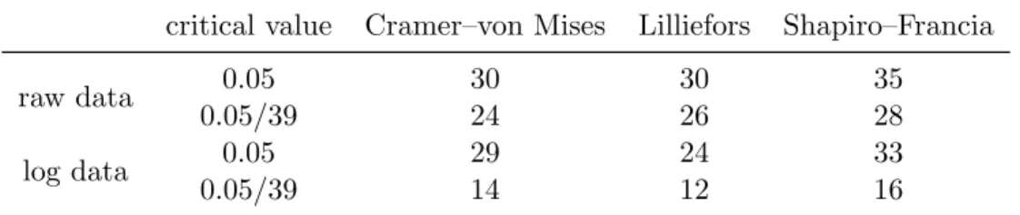
Although the normality assumption can be relaxed if we only focus on estimating a precision matrix, it plays an essential role in making the neat connection between a sparse precision matrix and a sparse Gaussian graphical model. Without normality, we ought to be very cautious when translating the output of a good sparse precision matrix estimation algorithm into an interpretable sparse Gaussian graphical model. However, the normality assumption often fails in reality. For example, the observed data are often skewed or have heavy tails. To illustrate the issue of non-normality in real applications, let us consider the gene expression data to construct isoprenoid genetic regulatory network in Arabidposis thaliana, which included 16 genes from the mevalonate (MVA) pathway in the cytosolic, 18 genes from the plastidial (MEP) pathway in the chloroplast, and also 5 encode proteins in the mitochondrial. The data, initially used by Wille et al. (2004), contained the gene expression measurements of 39 genes assayed on n = 118 Affymetrix GeneChip microarrays. For more details about the data, we refer readers to Wille et al. (2004) and Gilbert et al. (2009). This dataset was later re-analyzed by Li and Gui (2006); Drton and Perlman (2007) and Gilbert et al. (2009) in the context of Gaussian graphical modeling after taking the log-transformation of the expression data. However, the normality assumption may be inappropriate for this dataset even after the log-transformation. To show this, we conduct the normality test at the significance level of 0.05 as in Table Table 3.1, it is clear that at most 9 out of 39 genes would pass any of three normality tests, and even after log-transformation, at least 60% genes reject the null hypothesis of normality. Under Bonferroni correction there are still over 30% genes that fail to pass any normality test. Figure Figure 3.1 plots the histograms of two key isoprenoid genes MECPS in the MEP pathway and MK in the MVA pathway after the
log-Table 3.1: Testing for Normality of the gene expression data in the Arabidposis thaliana data. This table illustrate the number out of 39 genes rejecting the null hypothesis of normality at the significance level of 0.05.
critical value Cramer–von Mises Lilliefors Shapiro–Francia
raw data 0.05 30 30 35 0.05/39 24 26 28 log data 0.05 29 24 33 0.05/39 14 12 16 Histogram of log(MECPS) Expression Frequency 7.0 7.5 8.0 8.5 9.0 0 5 10 15 Histogram of log(MK) Expression Frequency 3 4 5 6 7 0 5 10 15 20
Figure 3.1: Illustration of the non-normality after the log-transformation preprocess-ing in the isoprenoid gene expression data.
transformation preprocessing, clearly showing the non-normality of the data after the log-transformation.
Using transformation to achieve normality is a classical idea in statistical mod-eling. The celebrated Box-Cox transformation is widely used in regression analysis. However, any parametric modeling of the transformation suffers from model mis-specification which could lead to misleading inference results. In this chapter we take a nonparametric transformation strategy to handle the non-normality issue. Let F(·) be the CDF of a continuous random variableX and Φ−1(·) be the inverse of the CDF
is easy to see that Z is standard normal regardless of F. Motivated by this simple probabilistic result, we consider modeling the data by the nonparanormal model:
The nonparanormal model: X = (X1,· · · , Xp) follows a
nonpara-normal distribution if there is a vector of unknown univariate monotone increasing transformations, denoted by f = (f1,· · · , fp), such that the
transformed random vector follows a multivariate normal distribution with mean 0 and covariance Σ:
f(X) = (f1(X1),· · · , fp(Xp))∼Np(0,Σ), (3.1)
where without loss of generality the diagonals of Σare all equal to 1.
Note that model (3.1) implies that fj(Xj) is a standard normal random variable.
Thus, fj must be Φ−1 ◦Fj where Fj is the CDF of Xj. Since the marginal
normal-ity can be always achieved by transformations, model (3.1) basically assumes that after transformation those marginally normal distributed variables also follow a joint normal distribution. Define Z = (Z1, . . . , Zp) = (f1(X1),· · ·, fp(Xp)). By the joint
normality assumption ofZ, we know thatθij = 0 if and only ifZi ⊥⊥Zj|Z\ {Zi, Zj}.
Interestingly, we have that
Zi ⊥⊥Zj| Z\ {Zi, Zj} ⇐⇒Xi ⊥⊥Xj| X \ {Xi, Xj}.
Therefore, a sparse precision matrixΘcan be directly translated into a sparse graph-ical model for presenting the original variables. In other words, the nonparanormal model nicely retains the good interpretability of the Gaussian model. We follow Liu et al. (2009) to call model (3.1) the nonparanormal model, but model (3.1) is in fact a semiparametric Gaussian copula model. The semiparametric Gaussian copula model is a nice combination of flexibility and interpretability. Semiparametric Gaussian
cop-ulas have generated a lot of interests in statistics, econometrics and finance (Klaassen and Wellner, 1997; Song, 2000; Tsukahara, 2005; Chen and Fan, 2006). Much of the existing theoretical work on the inference of semiparametric Gaussian copulas focuses on the classical asymptotic setting where the dimension is fixed and the sample size goes to infinity.
In this work we primarily focus on estimating Θwhich is then used to construct a nonparanormal graphical model. As for the nonparametric transformation function, by the expression fj = Φ−1◦Fj, we have a natural estimator for the transformation
function of the jth variable as ˆfj = Φ−1 ◦Fˆj+ where ˆF
+
j is a Winsorized empirical
CDF of the jth variables. Note that the Winsorization is used to avoid infinity value and to achieve better bias-variance tradeoff; see Liu et al. (2009) for detailed discus-sion. In this chapter we show that we can directly estimate Θ without estimating these nonparametric transformation functions at all. This statement seems to be a bit surprising because a natural estimation scheme is a two-stage procedure: first esti-matefj and then apply a well-developed sparse Gaussian graphical model estimation
method to the transformed data ˆzi =fˆ(xi),1≤i≤n. Liu et al. (2009) have actually
studied this “plug-in” estimation approach. They proposed a winsorized estimator of the nonparametric transformation function and used the Graphical LASSO in the second stage. They established convergence rate of the “plug-in” estimator when p is restricted to a polynomial order of n. However, the “plug-in” approach does not yield a satisfactory rate of convergence, for the rate of convergence can be established for the Gaussian graphical model even whenpgrows withnalmost exponentially fast (Ravikumar et al., 2008). As noted in Liu et al. (2009), it is very challenging to push the theory of the “plug-in” approach to handle exponentially large dimensions. The “plug-in” estimator has a much slower rate of convergence, largely due to the fact that it requires uniform convergence over p nonparametric functions in order to ensure a certain rate of convergence for estimating Θ, which was proved only for polynomial
large dimensions in Liu et al. (2009). One might ask if using a better estimator for the transformation functions could improve the rate of convergence such that pcould be allowed to be nearly exponentially large relative to n. This is a legitimate direction for research. We do not pursue this direction in this work. Instead, we show that we could use a rank-based estimation approach to achieve the exact same goal without estimating these transformation functions at all.
Our estimator is constructed in two steps. First, we propose a nonparametric rank-based sample estimate of Σand prove its rate of convergence under the matrix entry-wise `∞ norm. As the second step, we compute a sparse estimator Θfrom the
rank-based sample estimate of Σ. For that purpose, we consider several regularized rank estimators, including the rank-based Graphical LASSO, the rank-based neigh-borhood Dantzig selector and the rank-based CLIME. The complete methodological details are presented in Section 3.2. In Section 3.3 we establish theoretical properties of the proposed rank-based estimators regarding both precision matrix estimation and graphical model selection. Section 3.4 contains simulation results and the rank-based analysis of the isoprenoid genetic regulatory network. Section 3.5 contains the concluding remarks, and technical proofs are presented in the Appendix B.
3.2
Proposed Methodology
We first introduce some necessary notation. For a matrix A = (aij), we define its
entry-wise `1 norm as kAk1 =
P
(i,j)|aij|, and its entry-wise `∞ norm as kAkmax =
max(i,j)|aij|. For a vector v = (v1,· · · , vl), we define its `1 norm as kvk`1 =
P
j|vj|
and its`∞ norm askvk`∞ = maxj|vj|. To simplify notation, defineMA,B as the
sub-matrix of M with row indexes A and column indexes B, and define vA as the
sub-vector ofvwith indexesA. Let (k) be the index set{1, . . . , k−1, k+1, . . . , p}. Denote byΣ(k)=Σ(k),(k) the sub-matrix of Σwith both k-th row and column removed, and
denote by σ(k) = Σ(k),k the vector including all the covariances associated with the
k-th variable. In the same fashion, we can also define Θ(k), θ(k), and so on.
3.2.1
The oracle procedures
Suppose an oracle knows the underlying transformation vector, then the oracle could easily recover “oracle data” by applying these true transformations, i.e. zi =f(xi)
for 1≤i≤n. Before presenting our rank-based estimators, it is helpful to revisit the “oracle” procedures that are defined based on the “oracle data”.
• The oracle Graphical LASSO. Let Σˆo be the sample covariance matrix for the “oracle” data, and then the “oracle” log-profile-likelihood becomes
log det(Θ)−tr(ΣˆoΘ).
The “oracle” Graphical LASSO solves the following`1penalized likelihood
prob-lem: min Θ0−log det(Θ) + tr( ˆ ΣoΘ) +λX i6=j |θij|. (3.2)
• The oracle neighborhood LASSO selection. Under the nonparanormal model (3.1), for eachk = 1, . . . , p, the “oracle” variableZkgivenZ(k)is normally
distributed as NZT(k)Σ−(k1)σ(k),1−σT(k)Σ −1 (k)σ(k) ,
which can be equivalently written as
with
βk =Σ−(k1)σ(k) and εk∼N(0,1−σT(k)Σ
−1 (k)σ(k)).
Notice that βk and εk are closely related to the precision matrix Θ, i.e.
θkk = 1/Var(εk)
and
θ(k) =−βk/Var(εk).
Thus for the k-th variable,θ(k) andβkshare exactly the same sparsity pattern.
Following Meinshausen and B¨uhlmann (2006), the oracle neighborhood LASSO selection obtains the solution βˆok from the following LASSO penalized least squares problem, min β∈Rp−1 1 n n X i=1 (zik−zTi(k)β) 2+λkβk `1, (3.3)
and then the sparsity pattern of Θ can be estimated by integrating the neigh-borhood support set of βˆok= ( ˆβo
kj)j6=k, i.e. ˆnek ={j : ˆβkjo 6= 0} via intersection
or union.
We notice the fact that 1 n n X i=1 (zik−zTi(k)β) 2 =βTˆ Σ(ok)β−2βTσˆo(k)+ ˆσkko
Then (3.3) can be written in the following equivalent form
min
β∈Rp−1
βTΣˆo(k)β−2βTσˆo(k)+λkβk`1. (3.4)
• The oracle neighborhood Dantzig selector. Following Yuan (2010), the LASSO penalized least squares in (3.3) in the neighborhood approach can be replaced with the Dantzig selector as follows:
min β∈Rp−1 kβk`1 subject to k 1 n n X i=1 zi(k)(zTi(k)β−zik)k`∞ ≤λ. (3.5)
Then the sparsity pattern of Θ can be similarly estimated by integration via intersection or union. Furthermore, we notice that
1 n n X i=1 zi(k)(zTi(k)β−zik) = Σˆ o (k)β−σˆ o (k).
Then (3.5) can be written in the following equivalent form
min β∈Rp−1 kβk`1 subject to kΣˆ o (k)β−σˆ o (k)k`∞ ≤λ. (3.6)
• The oracle CLIME. Following Cai et al. (2011) we can estimate sparse pre-cision matrices by solving a constrained `1 minimization problem:
arg min
Θ kΘk1 subject to k
ˆ
ΣoΘ−Ikmax≤λ. (3.7)
Cai et al. (2011) compared the CLIME and the Graphical LASSO and show that the CLIME enjoys nice theoretical properties without assuming the irrep-resentable condition of Ravikumar et al. (2008) for the Graphical LASSO.
3.2.2
The proposed rank-based estimators
The existing theoretical results in the literature can be directly applied to these oracle estimators. However, the “oracle data” z1,z2, . . . ,zn are unavailable and thus the
above-mentioned “oracle” procedures are not genuine estimators. Naturally we wish to construct a genuine estimator that can mimic the oracle estimator. To this end, we can derive an alternative estimator of Σbased on the actual data x1,x2, . . . ,xn and
then feed this genuine covariance estimator to the Graphical LASSO, the neighbor-hood selection or CLIME. To implement this natural idea, we propose a rank-based estimation scheme. Note that Σ can be viewed as the correlation matrix as well, i.e. σij = corr(zi,zj). Let (x1i, x2i, . . . , xni) be the observed values of variable Xi. We
convert them to ranks denoted by ri = (r1i, r2i, . . . , rni). Spearman’s rank
correla-tion ˆrij is defined as Pearson’s correlation between ri and rj, i.e. ˆrij = corr(ri,rj).
Spearman’s rank correlation is a nonparametric measure of dependence between two variables. It is important to note that ri are the ranks of the “oracle” data.
There-fore, ˆrij is also identical to the Spearman’s rank correlation between the “oracle”
variables Zi, Zj. In other words, in the framework of rank-based estimation, we can
treat the observed data as the “oracle” data and avoid estimating p nonparametric transformation functions.
The nonparanormal model implies that (Zi, Zj) follows a bivariate normal
distri-bution with correlation parameter σij. Then a classical result due to Kendall (1948)
shows the relationship between σij and ˆrij is as follows
lim n→+∞E(ˆrij) = 6 πarcsin( 1 2σij), (3.8)
(1948) suggested using the adjusted Spearman’s rank correlation
ˆ
rsij = 2 sin(π
6ˆrij). (3.9)
Combining (3.8) and (3.9) we see that ˆrs
ij is an asymptotically unbiased estimator
![Table 2.3: Application to HIVRT data. NSE is the number of “stable edges”. E[V ] is the expected number of falsely selected edges](https://thumb-us.123doks.com/thumbv2/123dok_us/800730.2601186/37.918.182.792.161.324/table-application-hivrt-number-stable-expected-falsely-selected.webp)