Implementing Deep Learning Techniques in 5G IoT Networks for 3D Indoor Positioning: DELTA (DeEp Learning-Based Co-operaTive Architecture)

Article

Implementing Deep Learning Techniques in 5G IoT

Networks for 3D Indoor Positioning: DELTA (DeEp

Learning-Based Co-operaTive Architecture)

Brahim El Boudani1,* , Loizos Kanaris2, Akis Kokkinis2 , Michalis Kyriacou3, Christos Chrysoulas4 _{, Stavros Stavrou}3_{and Tasos Dagiuklas}1

1 _{Division of Computer Science and Informatics, London South Bank University, London SE1 0AA, UK;} [email protected]

2 _{Department of Electrical Engineering, Eindhoven University of Technology, 5612 AE Eindhoven,} The Netherlands; [email protected] (L.K.); [email protected] (A.K.) 3 _{Faculty of Pure and Applied Sciences, Open University of Cyprus, 2252 Nicosia, Cyprus;}

[email protected] (M.K.); [email protected] (S.S.)

4 _{School of Computing, Edinburgh Napier University, Edinburgh EH11 4DY, UK; [email protected]} * Correspondence: [email protected]

Received: 1 July 2020; Accepted: 22 September 2020; Published: 25 September 2020 Abstract: In the near future, the fifth-generation wireless technology is expected to be rolled out, offering low latency, high bandwidth and multiple antennas deployed in a single access point. This ecosystem will help further enhance various location-based scenarios such as assets tracking in smart factories, precise smart management of hydroponic indoor vertical farms and indoor way-finding in smart hospitals. Such a system will also integrate existing technologies like the Internet of Things (IoT), WiFi and other network infrastructures. In this respect, 5G precise indoor localization using heterogeneous IoT technologies (Zigbee, Raspberry Pi, Arduino, BLE, etc.) is a challenging research area. In this work, an experimental 5G testbed has been designed integrating C-RAN and IoT networks. This testbed is used to improve both vertical and horizontal localization (3D Localization) in a 5G IoT environment. To achieve this, we propose the DEep Learning-based co-operaTive Architecture (DELTA) machine learning model implemented on a 3D multi-layered fingerprint radiomap. The DELTA begins by estimating the 2D location. Then, the output is recursively used to predict the 3D location of a mobile station. This approach is going to benefit use cases such as 3D indoor navigation in multi-floor smart factories or in large complex buildings. Finally, we have observed that the proposed model has outperformed traditional algorithms such as Support Vector Machine (SVM) and K-Nearest Neighbor (KNN).

Keywords:5G IoT; indoor positioning; deep learning; tracking; localization; navigation; positioning accuracy; single access point positioning; Internet of Things

1. Introduction

In the era of 5G IoT [1], real-time positioning is becoming increasingly required by context-aware applications and location-based services. Typical scenarios include locating doctors and patients inside a hospital, advertising commercial products to mall visitors, monitoring gas and oil plants status, pinpointing dead crops in vertical farms, identifying victims’ location in Public Protection and Disaster Recovery (PPDR), etc. Moreover, several advanced applications can further provide cellular phone fraud detection, location-sensitive billing, as well as navigation from and to almost everywhere, through the utilization of heterogeneous wireless technologies, fusion of sensor and IoT data [2–5]. A recent report published by IEEE has estimated 50 billion [6] mobile devices will be connected to the Sensors2020,20, 5495; doi:10.3390/s20195495 www.mdpi.com/journal/sensors

cloud by the end of 2020. These devices will need constant access to data anywhere. Cisco has predicted that 26 billion [7] of these devices will be IoT or Wireless Sensor Network (WSN) devices. In this respect, technologies like Cloud Radio Access Network (C-RAN), Millimeter Wave (mm-Wave) communication, ultra dense communication [8], device-to-device (D2D) communication and Vehicle-to-everything (V2X) [9,10] and protocols like IEEE 802.11be (Extremely high Throughput WLAN) [11], IEEE 802.11az (Next Generation Positioning) [12] are not only introduced to increase the bandwidth of communication but also to offer the possibility of co-operative and precise localization. Additionally, with 5G paving the path for a seamless collaboration among heterogeneous wireless systems (cellular, WiFi, WSN, IoT, etc.), a great opportunity has risen in the area of indoor localization in urban areas under the framework of smart cities. Such high dense networks could be utilized to solve multi-agent positioning and offer agility and scalability for accurate positioning as a service. In this direction, we propose a DEep Learning-based with Co-operative Architecture (DELTA) algorithm to enhanced 3D indoor localization. The contributions of this paper can be summarized as follows:

• A realistic 3D indoor localization scenario for 5G IoT networks has been designed using an emulated 5G C-RAN and Zolertia IoT nodes.

• We present a novel approach to Received Signal Strength (RSS)-based fingerprint using 3D multi-layered radiomap to enhance the learning of network signal behaviour.

• A deep learning cooperative algorithm is implemented on the constructed multi-layered radiomap for an improved 3D localization indoor localization. The proposed method targets improving vertical and horizontal localization for use case scenarios such as indoor navigation or people tracking in multi-floor smart or large complex buildings. Based on the results of the emulated realistic radio-planning, we have shown how the DELTA outperformed KNN and SVM.

The remaining of this paper is organized as follows: Section2covers related research to this paper. Section3describes the problem related to indoor positioning in a 3D environment. Section4gives a detailed description of the underlying architecture of the DELTA model. Section5consists of a discussion and analysis of the performance results produced by our proposed approach compared with other traditional models. Lastly, Section6summarises a conclusion and spots possible future work. 2. Related Work

Indoor positioning techniques can be divided into two main categories: fingerprint and multilateration. In the latter, given a known propagation speed, the distance between a receiver and a group of transmitters is measured using techniques such as Direction of Arrival (DoA), Time of Arrival (TOA)/Time of Flight (TOF), Angle of Arrival (AoA), Time Difference of Arrival (TDOA) and Return Time of Flight (RTOF). These techniques are commonly used in Global Navigation Satellite Systems (GNSS) [13], such as Global Positioning System (GPS) and Galileo, but surprisingly they are also found in IoT indoor navigation solutions [14]. However, multilateration relies mainly on the travelling time or the direction of the signal rays. This makes indoor localization a complex task especially with many issues rising such as synchronization errors and multi-path fading [15–17].

In the fingerprint-based technique, a set of RSS measurements are taken and linked to specific Reference Points (RP) (also known as fingerprints or signatures). Localization using this approach works in two phases: offline and online. During the offline phase, a site survey is conducted with the purpose of linking the measured signal strength values to predefined RPs. The outcome of this measurements campaign is then stored in a radiomap database. During the online phase, a user equipment receives real-time signals and tries to match them with existing records stored in the radiomap database using a matching algorithm. In the context of IoT localization, the RSS signal is collected from wireless technologies such as Zigbee, LoRA, Wifi, Raspberry Pi, BLE, RFID. Since it does not require any specialised equipment or time synchronization to obtain the RSS signal, this technique is usually preferred to multilateration. For instance, authors in [18] have studied how robust localization for robots and IoT can be achieved using RSS fingerprint. Additionally, another interesting approach

has been introduced in [19] where the authors have focused on the use of IoT and Wifi-enabled devices to improve fingerprinting in an indoor environment. Recently, a new concept has been developed by Ali et al. [20] using raster maps instead of traditional offline scene analysis. Furthermore, a hybrid solution implemented on LoRa devices, which combines RSS fingerprinting with AoA methods is discussed in [14]. The proposed idea is very promising but it has inherited synchronization issues from multilateration. From these examples, it is undoubtedly clear that the RSS-based fingerprint method is widely used in the research community. This is due to improved localization and reduced computational complexity, as concluded by Amr et al. [19]. A detailed comparison of technologies and algorithms implementing the fingerprint technique for IoT indoor positioning has been carried out by [15,21–23].

In the fingerprint-based approach, deep learning techniques have been widely used to extract common patterns from a sparse radiomap database and to improve localization. In recent years, it has gained a huge popularity among the indoor localization researchers, in particular, due to its robustness and high accuracy [24]. Supervised and unsupervised deep learning algorithms have been recently implemented in 2D localization [25] and multi-floor localization [26]. Recently, Wafa et al. [27] studied the use of Convolutional Neural Networks (CNN) on IoT-Sensor System to determine the node location. In this simulation, the authors converted the 2D localization problem into a 3D image tensor identification problem. The 3D tensor has been constructed using a 2D matrix of RSS signals and 1D kurtosis. This concept has achieved 2 m average error accuracy but a similar system was also implemented in [28] and usually requires a large number of access points deployed in a small space to achieve this result. In [29], authors have implemented a Deep Belief Network (DBN) on an active RFID tag system for accurate location estimation. Their solutions consisted of a set of stacked Restricted Boltzmann Machine (RBM) layers called autoencoders trained using Contrastive Divergence with one-step iteration (CD-1). This algorithm has improved the 2D positioning. To achieve this, the authors have deployed a large number of RFID tags in a 12 m× 12 m indoor environment, which does not take into account the power consumption of the devices. Finally, Wang et al. [30] have suggested a hybrid deep learning solution combining a regression Deep Neural Network (DNN) with a Convolutional AutoEncode (CAE) using Visible Light Communication (VLC). To overcome the issue of fluctuated signal reading in the RSS-based fingerprint method, the authors have proposed an algorithm taking into account a set of consecutive signal readings and converting them to an RSS Temporal Image (RTI), instead of implementing the traditional RSS measurement processing technique. However, despite having been used in several works [31,32], VLC suffers from issues such as interference with other ambient lights, signal shadowing and usually requires the receiver to be in Line-Of-Sight (LOS), which can affect the accuracy of the location estimation. A detailed comparison of deep learning and other machine learning algorithms used in localization for IoT environment is covered in [33,34].

Until now, most of the existing IoT-based indoor localization solutions have mainly focused on either 2D localization or floor detection. However, in some special use cases scenarios such as indoor navigation for Unmanned Aerial Vehicle (UAV) or Automated Guided Vehicle (AGV) in a smart factory or big supermarket, precise 3D positioning is indispensable for daily operations. To address this issue, we suggest the DELTA to maximize the localization accuracy and minimize the distance error in a 3D indoor environment.

3. System Model and 3D Localization Problem

In this section, we introduce our proposed system model using Deep Neural Networks (DNN) and multi-layered radiomap to perform 3D Indoor Localization. To the best of our knowledge, this is a novel approach to implement deep learning on multi-layered radiomap for localization purposes. The main benefit of the proposed method is improved localization accuracy, and computational complexity minimization during online fingerprinting through the adoption of deep learning techniques, while at the same time utilizing the widely spreading WSN and/or IoT infrastructure making it an economical

solution. To realize these steps, we considered N to be the number of transmitters in the environment and x, y and z, the corresponding coordinates of each fingerprint entry on the constructed radiomap. The 3D multi-layered fingerprint database has been constructed by linking the RSS values received from the transmitters to a 3D location on the radiomap [35]. This can be mathematically expressed as:

M={(L1,S1),(L2,S2), . . . ,(Ln−1,Sn−1),(Ln,Sn)} (1) whereMis the ratio-map database,S∈ _RNXM_{is a vector of RSS signal values and L is a vector of} three values:L≡ {x,y,z}andLnrepresents the total number of the sample location ofxn,ynandzn associated with each signal vector sampleSncollected during the offline-phase.

In this respect, the estimation problem is defined by solving the 3D localization problem using a matrix of historical location points and their corresponding signal values. However, the challenge is to model the non-arbitrary relationships betweenNtransmitters members ofSsignal matrix to predict accurately the 3D location L using a deep learning algorithm. To achieve this, the 3D localization has been segmented to two sets of problems:

Problem 1. Given a matrix of S signal sent from N transmitters, predict the x and y coordinates of a 2D mobile station location. This can be written as:

λ1= f(S¯ij) (2) whereλ1 represents the xi and yi 2D location, which we would like to estimate, and f(Sij)represents the function that utilizes RSS values received by the transmitters to predict the location of the mobile station. Problem 2. Given a matrix of S signal sent from N transmitters to the mobile station and xi, yi, known from problem 1, estimate the zicoordinate. This can be mathematically expressed as:

λ2= f(S¯ij,λ1) (3) whereλ2is the zilocation,λ1is the output of problem 1 solution and Sijrepresents a matrix of signal values S as previously stated in problem 1.

4. DELTA 3D Localization for 5G WSN Network

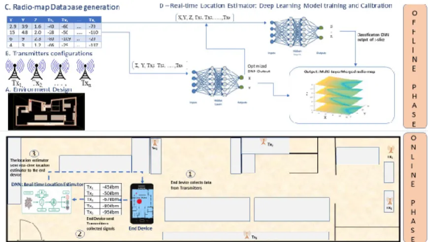
In this section, the DELTA System has been developed for 3D multi-layered indoor environment localization. Figure 1depicts the steps undertaken to realize a co-operative system for accurate 3D prediction.

4.1. Test Environment Description

In this subsection, we describe the test environment. The area of interest is a typical laboratory, with open spaces as well as private rooms defined by the following dimensions: 8 m width×16 m depth×2.75 m height. The lab environment was dynamic during this experiment.

4.1.1. Step I: The Physical Network Setup

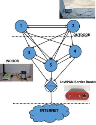
For the physical setup, an indoor test environment was deployed where a 5G network was emulated by a typical IoT network with Zolertia RE-Mote Revision B nodes connected to a LoWPAN Border Router, as illustrated in Figure2.

Figure 2.Network setup topology.

We randomly placed 5 Zolertia nodes, with their antennas at vertical polarization, as shown in Figure2. The nodes and the ray tracing propagation mechanisms have been configured as per Tables1and2.

Table 1.Wireless Sensor Network (WSN) and radio propagation parameters.

Parameter Value

Rx sensitivity (dBm) −120

Tx power (dBm) 3

antenna Type omni

Max refractions 12

Max reflections 12

Max diffractions 1

4.1.2. Step II: Connecting IoT to 5G C-RAN

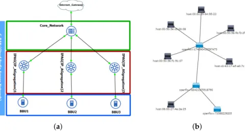
To simulate the 5G WSN environment, each Zolertia node was connected to an experimental 5G C-RAN. The setup was built using a GNS3 network simulator [36] and OpenDaylight Software Defined Controller [37]. These two can control the network setup behaviour at the network layer level. Figure3shows a setup built using a GNS3 network simulator and a Software Defined Controller OpenDaylight dashboard for the network topology. These two elements can control the network setup behaviour at the network layer level.

(a) (b)

Figure 3.5G C-RAN setup on GNS3 and WSN Network Connected to OpenDaylight SDN Controller. (a) 5G emulated C-RAN testbed on GNS3; (b) WSN and GNS3 emulated 5G C-RAN connected on OpenDaylight.

4.1.3. Step III: Simulating the Test Environment

Using a 3D deterministic simulator called TruNET Wireless [38], we constructed a multi-layered fingerprint radiomap dataset, in order to conduct the offline training phase, as illustrated in Figure1. During this procedure, in addition to the network setup configuration, the constitutive parameters of all environment object materials were also configured as per Table2, in order to retrieve realistic results [39]. The benefits of utilizing a deterministic simulation are to construct radiomaps instead of launching measurement campaigns as analysed in [40]. The summary of correlation results of this study is covered in Section5. The simulation environment for this study is shown in Figure4.

Table 2.Material constitutive parameters of the test environment.

Material El. Per. (F/m) L. Tangent

Concrete 3.9 0.23 Wood 2 0.025 Brick 5.5 0.03 Metal 1 1,000,000 Plasterboard 3 0.067 Glass 4.5 0.007

4.1.4. Physical Network Behaviour

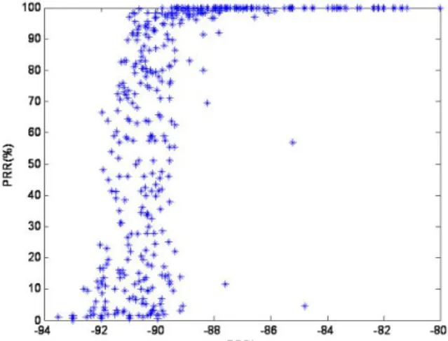
The signal propagation can be affected by various factors leading to the degradation of the signal quality especially in low power radio networks such as Wireless Sensor Networks. For a successful simulation, it is always crucial to observe the physical network behaviour during the offline measurement campaign. The effects of the physical layer and the various factors contributing to changes in the environment have been extensively studied in [41]. Using Link Quality Estimation (LQE) metrics such as Packet Reception Ratio (PRR) and Signal-to-Noise-Ratio (SNR), Baccour et al. [41] have studied the factors affecting a transmitter chip similar to that used in this experiment. It is very crucial to note that the simulated environment can be affected by various changes happening at the physical network. For the nodes used in this simulation, Figure5shows how the change in the Received Signal Strength Indicator (RSSI) can affect the PRR.

Figure 5.Packet Reception Ratio (PRR) vs. Received Signal Strength Indicator (RSSI) Signal CC2420 chip Baccour et al. [41].

Sometimes, measurement campaigns can be affected by various environmental noises, which may lead to unrealistic readings, either due to signal spikes or fluctuations. This noise can be either thermal noise or interference from other people’s equipment operating at the same frequency. To ensure signal samples obtained from TruNET Wireless are realistic, Figure6depicts the RSS coverage correlation analysis experiment conducted in [42]. The samples have been collected from Zolertia nodes over a week period at different instances with an interval of 15 min for each sample. The produced measurements for each RP have been averaged using the mean value. During this experiment, the IoT nodes have always been fixed and the environment was dynamic with people moving around.

Finally, it is clearly indicated that the simulated RSS values from the TruNET wireless simulator highly approximates the measured ones reaching a correlation level of more than 73%.

4.2. DELTA Architecture

Deep learning is a fundamental building block of the proposed architecture. It allows computational models consisting of multiple processing layers to learn the representation of data within multiple abstract levels [43]. One of the most important elements of deep learning is deep neural networks. Bengio et al. [44] refer to this as either deep feed forward networks or Multiple Layers Perceptron (MLP) since they have more than two hidden layers.

Our proposed architecture, as illustrated in Figure7, consists of two deep neural networks. The first is a regression modelδ1used to predict the 2D location of a mobile device. The second is a classification model referred to asδ2. Figure7illustrates the number of layers, neuron, input and

output parameters used for both models. Based on numerous trials and hyper-parameters tuning, we observed that three hidden layers were the best fit model for both networks.

Figure 6.RSS Values Measured vs. TruNET Kanaris et al. [42].

(δ1) (δ2)

Figure 7.Layers of DELTA Architecture Network. 4.3. DELTA Layers

4.3.1. Input Layers

Forδ1, the input is a transposed vector of RSS signals that can be expressed as follows: S =

[s1,s2, . . . ,sn]T. Forδ2, the input is slightly different toδ1. It consists of RSS signal inputSand the

output ofδ1. Each observation has a set of signals and predicted locations. This can be written as:

δ2_input=S∪(Lx,Ly) (4)

where S is the signal and Lx,Ly are the corresponding x and y locations. These two values are approximated usingδ1, as shown in Figure7.

4.3.2. Hidden Layers

Each element of this input gets multiplied by its specific weight vector~wand the product is added to a biasb. For the first hidden layer, this is expressed as follows:

h1=

n

∑

whereIi is an element from the input vector. EachIirepresents an input from a transmitter in the constructed fingerprint database. A summation of all these inputs is then fed to an activation unit A. In this case, the type of activation function used is a called Rectified Linear Unit (ReLu).

A1=max(0,h1) (6)

whereA1is an activation unit for the first hidden layer. The output of this hidden layer is the number of hidden neurons specified in the first hidden layer. Similarly, Equation (7) for hidden layer 2 is expressed as follows: h2= n

∑

This result is then fed into a further activation unitA2:

A2=max(0,h2) (8)

The hidden layer three receives the output of Equation (8) and makes similar calculations toh2:

h3=

n

∑

w3_ia2_i +b3_i (9)

Finally, the results returned in Equation (9) are fed into the activation unitA3.

A3=max(0,h3) (10)

4.3.3. Output Layers

Forδ1model, since the desired output is a real-valued number, a linear function has been applied using the following equation:

g(y= j|ai) = n

∑

w4_ia3_i +ei (11)

Forδ2model, the output is multiple class labels, therefore the Softmax function equation below has been used:

θ(ai) =

exp(a3 i)

∑jexp(a3j)

(12) To get the best final approximation,δ1supportsδ2. Algorithm1explains how both networks

cooperate to make a final localization.

Algorithm 1:DELTA Algorithm for 3D Localization

Input :RSS .Get Signal Vector

Output :3D Location

Require:Signal UpperThresholdη;

Require:Signal LowerThresholdµ;

forRSSiin RSSdo r← RSSi−µ

µ−η .Normalize signal

2D←δ1(r) .Apply first model prediction

1D←δ2(r,δ1) .Apply second model prediction

3D←2D∪1D .mergeδ1andδ2results

endfor

4.4. Prepossessing

4.4.1. Fingerprints Radiomap Database

As previously mentioned, we began by constructing the radiomap database using eight features. Table3gives a detailed explanation of each variable.

Table 3.The features used to construct the fingerprints database.

Variable Min. Value Max. Value Type

X 0 8 coordinates Y 0 16 coordinates Z 0.25 1.75 coordinates AP1 −120 dBm −28 dBm RSS value AP2 −100 dBm −30 dBm RSS value AP3 −100 dBm −40 dBm RSS value AP4 −90 dBm −50 dBm RSS value AP5 −100 dBm −60 dBm RSS value

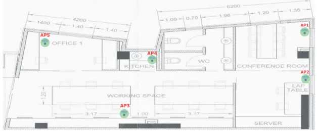
The constructed radiomap consists of 2880 3D References Points (RPs) associated with RSS values from five different WSN Access Points(APs). Each AP is placed at least three meters away. The position of these APs is shown on the lab floor-plan illustrated in Figure8.

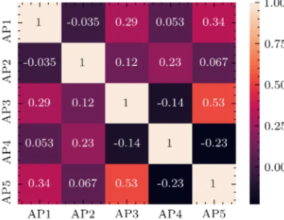
To ensure that there is no redundancy in the information collected, a Pearson correlation test has been conducted between each AP and the result is shown in Figure9. There is clearly no high negative or positive correlation between the APs used in this experiment.

In addition to this, Figure 10 shows each layer on the radiomap database constructed is significantly different from the other layer. The Figure shows the signal at 0.25, 0.75 and 1.75 m for Access Point 1.

Figure 8.Access points position on the setup environment floor-plan. 4.4.2. One-hot Encoding

One-hot encoding is one of the most common techniques for converting a token into a vector [45]. The conversion is achieved by associating each unique integer with every unique value from the column z. This turns every unique value into a binary vector having the size of the unique values. As a result, every column will have zero except for where the unique value has occurred. In our case, we have used the steps followed in Algorithm2to one-hot encode our target variable:

Algorithm 2:One hot Encoding

Input :Column Z .get Z columns

Output :Result Matrix of N binary vectors unique values from Z DictionaryD=[];

ResultsR={[],[],[],[]}; fori in Z.lengthdo

if i6∈D: .If value not in dictionary add it

key=D[i] D[i]=Z[i] endfor returnD

Map D into results R columns as binary vector {[Z1],[Z2], . . . ,[Zn]}

Figure 9.WSN access points correlation matrix.

4.4.3. Min–Max Normalization

Min–Max normalization has been implemented to make sure the learning of signal representation data is faster for DELTA architecture models to converge quickly. This concept works by fitting the original data into a new scale between 0 and 1. After this numeric transformation, the highest value becomes close to 1 and the lowest value is close to 0 as stated in [46]. The formula used to achieve this, is the following:

RSSi−min(RSS)

min(RSS)−max(RSS) (13)

where min(RSS) represents the values minimum threshold signal specified during the training signal, i.e., −120 dBm and max(RSS) represents the maximum value measured, i.e., −30 dBm. Each signal measurement we want to convert is denoted byRSSiwhereiis theithrow in N Transmitter. For other scenarios, it is advisable to use the receiver sensitivity level as the minimum value and the strongest measured signal during the offline-phase as the maximum value.

4.5. Hyper-Parameters Fine-Tuning 4.5.1. Loss Functions

• Using Euclidean Distance as loss function forδ1 model, the purpose is to train the model to minimize the Mean Euclidean Distance (MED) error between the actual and the predicted location.

D(Lact,Lpred) = 1 M m

∑

(xact_j −x_jpred)2_{+ (y}act j −y

pred

j )2 (14)

Lacthere denotes the actual location andLpreddenotes the predicted location.

• For the δ2 model, Categorical Cross-entropy is implemented as a loss function. This can be written as: H(Lact,Lpred) =− M

∑

∑

(z_ijAct·log(z_ijpred) (15)

whereLactdenotes the actual location andLpreddenotes the predicted location. Whilezijdenotes the ith observation in thejth z output class or level.

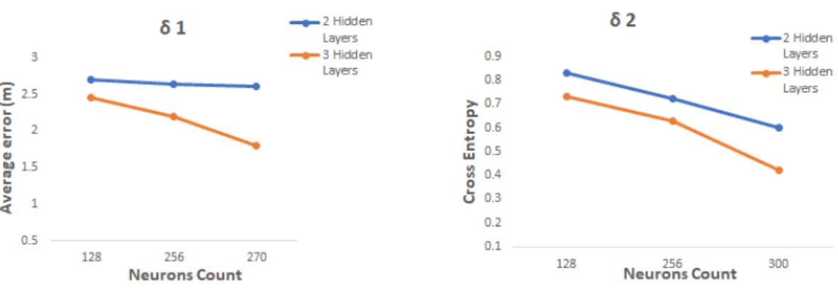
4.5.2. Hidden Layers and Neurons Size Determination

The number of hidden layers and neurons count used in the DELTA has been determined using the loss function specified the previous subsection. Figure11shows the performance of each network for each neuron count and layers number selected. As demonstrated in this figure, the categorical cross entropy loss is minimized after a third hidden layer has been added and the neurons count has been set to 300. Similarly, the average error was decreased in delta one after the parameters were changed to 300 neurons and three hidden layers.

Figure 11.The number of hidden layers and neurons vs. each loss function. 4.5.3. Batch Normalization

A batch is the number of samples propagated through the neural network model before the parameters are updated. To train each neural network faster, we have supported each layer with a batch normalization. This sort of normalization is applied to input samples of the same batch size. This fine-tuning technique has been proven to speed up the training and learning process by 12 times faster than the normal architecture as described by authors in [47]. The formula for the batch normalization implemented on each Deep Neural Network of DELTA system is:

Ti=

(Ti−µ(T)

p

σ2(T) +e

(16)

whereTis training batch,µ(T)is its mean,σ2(T)is its variance andeis a small constant number

added to support the variance. For this to work in Keras deep learning library [45], a layer of batch normalization with explicit parameters has to be added at the beginning of each hidden layer. 4.5.4. Regularization

To avoid overfitting, a regularization technique has been implemented to switch off certain neurons for some layers. This technique is called dropout. Details for this technique are provided by Nitish et al. in [48]. The dropout rate used in DELTA is 0.20 as suggested by [48]. After experimentation, we have concluded that for better results are achieved when implementing batch normalization before dropout.

4.6. Optimization

Optimization is the process of training a network using mini-batches and iterations to get the optimum configuration for its parameter. One of the widely used stochastic optimization algorithms in deep learning is ADAptive Momentum (ADAM). The algorithm can be viewed as a combination of RMSprop and Momentum [49]. It works by correcting the bias b and the weight w after each iteration. To get the best results from ADAM’s parameters, we specified a learning rateα=0.001,β1= 0.9 for the momentum control,β2= 0.99 for squared weight in RMSprop section ande=10−8as specified

by the authors in [49]. To implement this in Keras, ADAM parameters have to be specified before the model is compiled.

4.7. Scoring

Using 900 hidden neurons and three hidden layers, we have constructed modelδ1to predict x and y locations. This has yielded 279,302 parameters to be trained. Our cost function is the euclidean distance difference between each predicted observation and the original location. To minimize it, hyper-parameters have been fine-tuned such as the batch sizes and the number of times an

algorithm will iterate through an entire training dataset. One iteration is referred to as epochs. The aforementioned methodology resulted in an average positioning error of 1.6 m average (less than 2 m error overall) in both training and validation phases. Figure12shows how theδ1model mean Euclidean distance error in meters decreases over the number of epochs chosen, in this case 3000 epochs. However, by the end of epoch 3000, the model has converged and stopped improving its accuracy.

Figure 12.δ1Model mean Euclidean distance error in meter (m) vs. the number of Epochs.

Similarly, after an iterative tweaking of the architecture parameters, using 810 number of neurons and three hidden layers, we have constructed model delta 2 where z layer is the target variable. A total number of 235,592 parameters were trained in this model. The cost function is the multi-categorical cross entropy, which is used widely for classification scoring. Figure13shows how the categorical cross-entropy has been minimized after 2500 epochs.

Figure 13.δ2Categorical cross-entropy vs. the number of Epochs.

5. Performance Evaluation Results

In this section, we explore, evaluate and critically analyse the simulation results against famous industry methods such as SVM and KNN. However, before going through the results analysis, it is worth mentioning that KNN and SVM modelling tasks have been carried out using Scikit-learn [50], a widely used Python library toolset for machine learning and statistics. More specifically, SVM models have developed using an SVM class from the Scikit-learn library and KNN models have been built using a classifier class called KNeighborsClassifier [51]. The DELTA models have been constructed using Keras API [52], a deep learning library also available in Python. During the evaluation phase,

the three algorithms were implemented using python software on the same machine with Intel [email protected] CPU and 16 GB of RAM. In terms of time complexity, KNN has finished after 230 ms while SVM has taken 450 ms. The proposed DNN has used 160 ms to execute, making it more efficient than KNN and SVM.

5.1. Results Analysis 5.1.1.δ1s. KNN and SVM

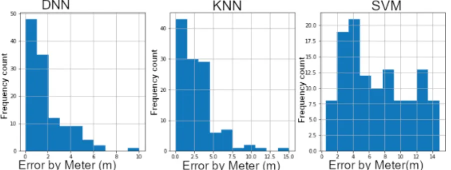
Using 180 random samples [39], we have bench-marked and assessed DNN modelδ1against KNN and Support Vector Regression (SVR) models. The samples have been obtained for each z layer making a total of 540 RPs. The SVR has been trained using a linear kernel, a degree of one and an epsilon value of one using 80% training and 20% validation data sets. Similarly, a KNN model has been trained with a K value set to three. The results in Figure14show the error distribution in meters for all three models. SVR has scored a rather worse error distribution where the peak of its distribution ranges between 4 and 6 m error. KNN has done slightly better compared to SVR. However, a large proportion of the distribution error falls between 3 and 5 m, which makes it the second worse performing after SVR. DNNδ1has performed better. The peak of its distribution error samples falls between zero and two meters with a mean error of 1.6 m. A detailed result is provided in Table4.

Figure 14.δ1vs. K-Nearest Neighbor (KNN) vs. Support Vector Regression (SVR).

Table 4.Frequency Count of Distance error (m) for each model.

DNN KNN SVM

Less Than 2 m 79 51 9

Between 2 m and 7 m 39 64 60

More than 7 m 2 5 51

5.1.2.δ2s. KNN and SVM

Using the aforementioned samples, the z layer (z coordinate) has been estimated. The results are depicted in Figure15 illustrating a visual comparison of each classifier in a bar-chart using misclassification count as a measure. Each model has been given an equal number of three classes 0.25, 1.25 and 1.75 m. At first glance, Figure15shows that Support Vector Classifier (SVC) has performed very badly in terms of classification of observations. The model has failed to accurately classify during the online phase. More than 66%—circa 120 samples—have been wrongly classified. With a total of 40 misclassified samples, K-Nearest Neighbor (KNN) has performed better than SVC but still does not differentiate between certain classes properly. Our proposedδ2model of DNN, has made excellent classification compared to both later models. As an effect, 100% of the 0.25 m layer has been accurately classified while more than 95% of the other two classes, 1.25 and 1.75 m, have also been properly predicted. The total number of misclassified samples is 20 bringing the classification accuracy rate to 89%. This shows how the proposed 3-D multi-layered model has outperformed the traditional models.

Table5gives a detailed count of each model and its misclassification count. The worse performing model is highlighted in red and the best performing model is highlighted in blue.

Figure 15.Model comparison:δ2vs. KNN vs. SVC. Table 5.Misclassification count for each model.

Model 0.25 m 0.75 m 1.75 m

DNN 10 10 0

KNN 20 11 9

SVC 60 57 3

6. Conclusions

In this work, we have proposed a novel approach for 3D Indoor Localization using DNN cooperative network algorithms implemented on 3D multi-layer radiomaps. To emulate a 5G infrastructure IoT indoor scenario, an IoT network is interconnected to an experimental 5G C-RAN. Using only an offline fingerprint database, we have also demonstrated how the proposed model has outperformed traditional industry models such as KNN. We have accurately implemented this model to the indoor environment. If the steps shown in Figures1and7are properly followed, a reliable and fast 3D localization can be achieved. This concept can also be further developed to cover more complex indoor positioning scenarios, involving radio data from a heterogeneous network (HetNEt) such as 5G microinfrastructure (Microcells, femtocell, picocells, etc.). Finally, the proposed DELTA model works very well with RSS based IoT and Wireless Sensor Networks. Thus, our future work will be improving the model by including information fused from other networks such as WiFi and Bluetooth Low Energy (BLE) and experimenting with more vertical layers. Another research direction could be adding floor level detection for buildings with multiple floors.

Author Contributions:All authors contributed equally to this work. All authors have read and agreed to the published version of the manuscript.

Funding:This work is supported by the HORIZON2020 H2020-MSCA-RISE-2016 European Framework Program, the SONNET project Consortium, Sigint Solutions Ltd., and London South Bank University. Self-Organization toward reduced cost and energy per bit for future Emerging radio Technologies with contract number 734545 Program.

Abbreviations

The following abbreviations are used in this manuscript: 3/2D 3/2 Dimensions

5G 5th Generation AoA Angle of Arrival ADAM ADAptive Momentum AP Access Points

BLE Bluetooth Low Energy C-RAN Cloud-Radio Access Network CAE Convolutional AutoEnconde

CD-1 Contrastive Divergence with one-step iteration CNN Convolutional Neural Networks

D2D device-to-device DBN Deep Belief Network

DELTA DEep Learning cooperaTive Architecture DNN Deep Neural Network

DoA Direction of arrival

GNSS Global Navigation Satellite System GPS Global Positioning System HetNet Heterogeneous Network IoT Internet of Things KNN K-Nearest Neighbor LOS Line-Of-Sight

MED Mean Euclidean Distance

MDPI Multidisciplinary Digital Publishing Institute MLP Multiple Layers Perceptron

mm-Wave Millimeter Wave

PPDR Public Protection and Disaster Recovery PRR Packet Reception Ratio

RP Reference Point

RSS Received Signal Strength

RSSI Received Signal Strength Indicator RTI RSS Temporal Image

RTOF Return Time of Flight SNR Signal-to-Noise-Ratio SVC Support Vector Classification SVM Support Vector Machine SVR Support Vector Regression TDOA Time Difference of Arrival TOA Time of Arrival

ToF Time of Flight V2X Vehicle-to-Everything VLC Visible Light communication WSN Wireless Sensors Networks References

1. Li, S.; Da Xu, L.; Zhao, S. 5G Internet of Things: A survey. J. Ind. Inf. Integr.2018,10, 1–9. [CrossRef] 2. Chen, M. Towards smart city: M2M communications with software agent intelligence. Multimed. Tools Appl.

2013,67, 167–178. [CrossRef]

3. Zhang, D.; Yang, L.; Chen, M.; Zhao, S.; Guo, M.; Zhang, Y. Real-Time Locating Systems Using Active RFID for Internet of Things.Syst. J. IEEE2014,10, 1–10. [CrossRef]

4. Ji, H.; Xie, L.; Wang, C.; Yin, Y.; Lu, S. CrowdSensing: A crowd-sourcing based indoor navigation using RFID-based delay tolerant network. J. Netw. Comput. Appl.2015,52, 79–89. [CrossRef]

5. Macagnano, D.; Destino, G.; Abreu, G. Indoor positioning: A key enabling technology for IoT applications. In Proceedings of the 2014 IEEE World Forum on Internet of Things (WF-IoT), Seoul, Korea, 6–8 March 2014; pp. 117–118. [CrossRef]

6. Yang, C.; Li, J.Interference Mitigation and Energy Management in 5G Heterogeneous Cellular Networks; IGI Global: Hershey, PA, USA, 2016.

7. Cisco Visual Networking Index: Global Mobile Data Traffic Forecast Update, 2017–2022. Available online:https://davidellis.ca/wp-content/uploads/2019/12/cisco-vni-mobile-data-traffic-feb-2019.pdf

(accessed on 28 July 2020).

8. Liu, Y.; Shi, X.; He, S.; Shi, Z. Prospective positioning architecture and technologies in 5G networks.

IEEE Netw.2017,31, 115–121. [CrossRef]

9. Wymeersch, H.; Seco-Granados, G.; Destino, G.; Dardari, D.; Tufvesson, F. 5G mmWave positioning for vehicular networks. IEEE Wirel. Commun.2017,24, 80–86. [CrossRef]

10. Bartoletti, S.; Conti, A.; Dardari, D.; Giorgetti, A. 5G Localization and Context-Awareness. Available online: https://www.5gitaly.eu/2018/wp-content/uploads/2019/01/5G-Italy-White-eBook-5G-Localization.pdf(accessed on 28 July 2020).

11. López-Pérez, D.; Garcia-Rodriguez, A.; Galati-Giordano, L.; Kasslin, M.; Doppler, K. IEEE 802.11 be Extremely High Throughput: The Next Generation of Wi-Fi Technology Beyond 802.11 ax.

IEEE Commun. Mag.2019,57, 113–119. [CrossRef]

12. Leonardo, L.; Yuhei, N.; Kurosaki, M.; Ochi, H. High Precision Localization Protocol with Diversity for 802.11 az. IEICE Tech. Rep. IEICE Tech. Rep.2017,117, 69–74.

13. Jaulin, L. 5-Instantaneous Localization. In Mobile Robotics; Jaulin, L., Ed.; Elsevier: Amsterdam, The Netherlands, 2015; pp. 171–196. [CrossRef]

14. Baik, K.J.; Lee, S.; Jang, B.J. Hybrid RSSI-AoA Positioning System with Single Time-Modulated Array Receiver for LoRa IoT. In Proceedings of the 2018 48th European Microwave Conference (EuMC), Madrid, Spain, 23–27 September 2018; pp. 1133–1136.

15. Zafari, F.; Gkelias, A.; Leung, K.K. A survey of indoor localization systems and technologies.IEEE Commun. Surv. Tutor.2019. [CrossRef]

16. McElroy, C.; Neirynck, D.; McLaughlin, M. Comparison of wireless clock synchronization algorithms for indoor location systems. In Proceedings of the 2014 IEEE International Conference on Communications Workshops (ICC), Sydney, Australia, 10–14 June 2014; pp. 157–162.

17. Boukerche, A.; Villas, L.A.; Guidoni, D.L.; Maia, G.; Cunha, F.D.; Ueyama, J.; Loureiro, A.A. A new solution for the time-space localization problem in wireless sensor network using uav. In Proceedings of the third ACM International Symposium on Design and Analysis of Intelligent Vehicular Networks and Applications, Barcelona, Spain, 3–8 November 2013; pp. 153–160.

18. Bae, Y. Robust Localization for Robot and IoT Using RSSI.Energies2019,12, 2212. [CrossRef]

19. Hilal, A.; Khalil, M.; Salman, A.; El-Tawab, S. Exploring the Use of IoT and WiFi-enabled Devices to Improve Fingerprinting in Indoor Localization. In Proceedings of the 2019 IEEE Global Conference on Internet of Things (GCIoT), Dubai, UAE, 4–7 December 2019; pp. 1–6.

20. Ali, M.U.; Hur, S.; Park, Y. Wi-Fi-based effortless indoor positioning system using IoT sensors. Sensors2019,

19, 1496. [CrossRef]

21. Njima, W.; Ahriz, I.; Zayani, R.; Terre, M.; Bouallegue, R. Comparison of similarity approaches for indoor localization. In Proceedings of the 2017 IEEE 13th International Conference on Wireless and Mobile Computing, Networking and Communications (WiMob), Rome, Italy, 9–11 October 2017; pp. 349–354. 22. Ding, G.; Zhang, J.; Tan, Z. Overview of received signal strength based fingerprinting localization in

indoor wireless LAN environments. In Proceedings of the 2013 5th IEEE International Symposium on Microwave, Antenna, Propagation and EMC Technologies for Wireless Communications, Chengdu, China, 29–31 October 2013; pp. 160–164.

23. Abualsaud, K.; Elfouly, T.M.; Khattab, T.; Yaacoub, E.; Ismail, L.S.; Ahmed, M.H.; Guizani, M. A survey on mobile crowd-sensing and its applications in the IoT era.IEEE Access2018,7, 3855–3881. [CrossRef] 24. Li, D.; Lei, Y.; Li, X.; Zhang, H. Deep Learning for Fingerprint Localization in Indoor and Outdoor

25. Passafiume, M.; Maddio, S.; Collodi, G.; Cidronali, A. An enhanced algorithm for 2D indoor localization on single anchor RSSI-based positioning systems. In Proceedings of the 2017 European Radar Conference (EURAD), Nuremberg, Germany, 11–13 October 2017; pp. 287–290.

26. Kim, K.S.; Lee, S.; Huang, K. A scalable deep neural network architecture for multi-building and multi-floor indoor localization based on Wi-Fi fingerprinting. Big Data Anal.2018,3, 4. [CrossRef]

27. Njima, W.; Ahriz, I.; Zayani, R.; Terre, M.; Bouallegue, R. Deep CNN for Indoor Localization in IoT-Sensor Systems. Sensors2019,19, 3127. [CrossRef]

28. Shao, W.; Luo, H.; Zhao, F.; Ma, Y.; Zhao, Z.; Crivello, A. Indoor positioning based on fingerprint-image and deep learning. IEEE Access2018,6, 74699–74712. [CrossRef]

29. Jiang, H.; Peng, C.; Sun, J. Deep Belief Network for Fingerprinting-Based RFID Indoor Localization. In Proceedings of the ICC 2019-2019 IEEE International Conference on Communications (ICC), Shanghai, China, 20–24 May 2019; pp. 1–5.

30. Wang, Z.; Zhang, X.; Wang, W.; Shi, L.; Huang, C.; Wang, J.; Zhang, Y. Deep Convolutional Auto-Encoder based Indoor Light Positioning Using RSS Temporal Image. In Proceedings of the 2019 IEEE International Symposium on Broadband Multimedia Systems and Broadcasting (BMSB), Jeju, Korea, 5–7 June 2019; pp. 1–5.

31. Tran, H.; Ha, C. Fingerprint-Based Indoor Positioning System Using Visible Light Communication—A Novel Method for Multipath Reflections. Electronics2019,8, 63. [CrossRef]

32. Kanaris, L.; Kokkinis, A.; Liotta, A.; Stavrou, S. Combining smart lighting and radio fingerprinting for improved indoor localization. In Proceedings of the 2017 IEEE 14th International Conference on Networking, Sensing and Control (ICNSC), Calabria, Italy, 16–18 May 2017; pp. 447–452.

33. Janssen, T.; Berkvens, R.; Weyn, M. Comparing Machine Learning Algorithms for RSS-Based Localization in LPWAN. In International Conference on P2P, Parallel, Grid, Cloud and Internet Computing; Springer: Berlin/Heidelberg, Germany, 2019; pp. 726–735.

34. Sinha, R.S.; Hwang, S.H. Comparison of CNN applications for RSSI-based fingerprint indoor localization.

Electronics2019,8, 989. [CrossRef]

35. Kaemarungsi, K. Efficient design of indoor positioning systems based on location fingerprinting. In Proceedings of the 2005 International Conference on Wireless Networks, Communications and Mobile Computing, Maui, HI, USA, 13–16 June 2005; Volume 1, pp. 181–186.

36. GNS3. Getting Started with GNS3|GNS3 Documentation. Available online:https://docs.gns3.com/docs/

(accessed on 28 July 2020).

37. OpenDaylight. Documentation Guide—OpenDaylight Documentation Magnesium Documentation. 2020. Available online:https://docs.opendaylight.org/en/stable-magnesium/documentation.html(accessed on 28 July 2020).

38. Fractal Networx Limited. TruNET Wireless. 2017. Available online:www.fractalnetworx.com(accessed on 28 July 2020).

39. Kanaris, L.; Kokkinis, A.; Fortino, G.; Liotta, A.; Stavrou, S. Sample Size Determination Algorithm for fingerprint-based indoor localization systems. Comput. Netw.2016,101, 169–177. [CrossRef]

40. Kanaris, L.; Kokkinis, A.; Liotta, A.; Stavrou, S. Quality of Fingerprint Radiomaps for Positioning Systems. In Proceedings of the 2017 24th International Conference on Telecommunications (ICT) (ICT 2017), Limassol, Cyprus, 3–5 May 2017.

41. Baccour, N.; Koubâa, A.; Mottola, L.; Zúñiga, M.A.; Youssef, H.; Boano, C.A.; Alves, M. Radio link quality estimation in wireless sensor networks: A survey. ACM Trans. Sens. Netw. (TOSN)2012,8, 1–33. [CrossRef] 42. Kanaris, L.; Sergiou, C.; Kokkinis, A.; Pafitis, A.; Antoniou, N.; Stavrou, S. On the Realistic Radio and

Network Planning of IoT Sensor Networks. Sensors2019,19, 3264. [CrossRef]

43. LeCun, Y.; Bengio, Y.; Hinton, G. Deep learning. Nature2015,521, 436. [CrossRef] [PubMed]

44. Goodfellow, I.; Bengio, Y.; Courville, A.Deep Learning; MIT Press: Cambridge, MA, USA; London, UK, 2016. 45. Chollet, F.Deep Learning with Python, 1st ed.; Manning Publications Co.: Greenwich, CT, USA, 2017. 46. Wye, K.F.P.; Kanagaraj, E.; Zakaria, S.M.M.S.; Kamarudin, L.M.; Zakaria, A.; Kamarudin, K.; Ahmad, N.

RSSI-based Localization Zoning using K-Mean Clustering. InIOP Conference Series: Materials Science and Engineering; IOP Publishing: Bristol, UK, 2019.

47. Ioffe, S.; Szegedy, C. Batch normalization: Accelerating deep network training by reducing internal covariate shift.arXiv2015, arXiv:1502.03167.

48. Srivastava, N.; Hinton, G.; Krizhevsky, A.; Sutskever, I.; Salakhutdinov, R. Dropout: A simple way to prevent neural networks from overfitting. J. Mach. Learn. Res.2014,15, 1929–1958.

49. Kingma, D.P.; Ba, J. Adam: A method for stochastic optimization.arXiv2014, arXiv:1412.6980.

50. Scikit-learn. 1.4. Support Vector Machines—Scikit-Learn 0.23.2 Documentation. Available online:https: //scikit-learn.org/stable/modules/svm.html(accessed on 8 December 2019).

51. Scikit-learn. Sklearn.Neighbors.KNeighborsClassifier—Scikit-Learn 0.23.2 Documentation. Available online:

https://scikit-learn.org/stable/modules/generated/sklearn.neighbors.KNeighborsClassifier.html

(accessed on 8 December 2019).

52. Keras. Keras API Reference. Available online:https://keras.io/api/(accessed on 8 December 2019).

c

2020 by the authors. Licensee MDPI, Basel, Switzerland. This article is an open access article distributed under the terms and conditions of the Creative Commons Attribution (CC BY) license (http://creativecommons.org/licenses/by/4.0/).