Classification of Breast Cancer Patients Using Somatic Mutation Profiles and Machine Learning Approaches

Theses & Dissertations Graduate Studies Fall 12-18-2015

Classification of Breast Cancer Patients Using Somatic Mutation

Classification of Breast Cancer Patients Using Somatic Mutation

Profiles and Machine Learning Approaches

Profiles and Machine Learning Approaches

University of Nebraska Medical Center

Follow this and additional works at: https://digitalcommons.unmc.edu/etd

Part of the Bioinformatics Commons, and the Systems Biology Commons

Recommended Citation Recommended Citation

Vural, Suleyman, "Classification of Breast Cancer Patients Using Somatic Mutation Profiles and Machine Learning Approaches" (2015). Theses & Dissertations. 50.

https://digitalcommons.unmc.edu/etd/50

This Dissertation is brought to you for free and open access by the Graduate Studies at DigitalCommons@UNMC. It has been accepted for inclusion in Theses & Dissertations by an authorized administrator of

CLASSIFICATION OF BREAST CANCER PATIENTS USING

SOMATIC MUTATION PROFILES AND MACHINE LEARNING

APPROACHES

by

Suleyman Vural

A DISSERTATION

Biomedical Informatics Graduate Program

Under the Supervision of Dr. Chittibabu Guda

University of Nebraska Medical Center Omaha, Nebraska

December, 2015

Supervisory Committee: Dr. James Eudy Dr. San Ming Wang Dr. Sanjukta Bhowmick Presented to the Faculty of

the University of Nebraska Graduate College in Partial Fulfillment of the Requirements

CLASSIFICATION OF BREAST CANCER PATIENTS USING SOMATIC MUTATION PROFILES AND MACHINE LEARNING APPROACHES

Suleyman Vural, Ph.D.

University of Nebraska Medical Center, 2015

Advisor: Chittibabu Guda, Ph.D.

The high degree of heterogeneity observed in breast cancers makes it very difficult to

classify cancer patients into distinct clinical subgroups and consequently limits the

ability to devise effective therapeutic strategies. In this study, we explore the use of gene

mutation profiles to classify, characterize and predict the subgroups of breast cancers.

We analyzed the whole exome sequencing data from 358 ethnically similar

breast cancer patients in The Cancer Genome Atlas (TCGA) project. Identified somatic

and non-synonymous single nucleotide variants were assigned a quantitative score (

C-score) that represents the extent of negative impact on the function of the gene. Using

these scores with a non-negative matrix factorization method, we clustered the patients

into three subgroups. By comparing the clinical stage of patients among the three

subgroups, we identified an early-stage-enriched and a late-stage-enriched subgroup.

Comparison of the C-scores (mutation scores) of these subgroups identified 358 genes

that carry significantly higher rates of mutations in the late-stage-enriched subgroup.

Functional characterization of these genes revealed important functional gene families

that carry a heavy mutational load in the late-state-enriched subgroup. Finally, using the

identified subgroups, we also developed a supervised classification model to predict the

help devise an effective treatment plan.

This study demonstrates that gene mutation profiles can be effectively used with

machine-learning methods to identify clinically distinguishable subgroups of cancer

patients. Genes and gene families that carry a heavy mutational load in

late-stage-enriched cancer patients compared to early-stage-late-stage-enriched subgroup were also identified

from functional analysis of genes. The classification model developed in this method

could provide a reasonable prediction of the stage of cancer patients solely based on

their mutation profiles. This study represents the first use of only somatic mutation

profile data to identify and predict breast cancer subgroups and this generic methodology

ACKNOWLEDGEMENTS

I wish to express my deepest gratitude and immeasurable appreciation to the following

people. Indeed, this work would not be possible without your help and support.

I would like to thank my advisor Dr. Chittibabu (Babu) Guda for all the helpful advice, continuous support, and guidance throughout my Ph.D. journey from

Albany to Omaha. I am grateful to my supervisory committee, Dr. James Eudy, Dr. San Ming Wang, and Dr. Sanjukta Bhowmick for their valuable guidance and suggestions. I am indebted to Dr. Xiaosheng Wang for his priceless help on my project. I would like to thank my dear friends in the Guda lab at UNMC for all the enjoyable

moments and stress relieving discussions. Those were truly invaluable and

unforgettable.

I would like to express my gratitude to the Turkish community in Omaha;

their help meant a lot to me. I greatly appreciate all the fruitful discussions we had,

which taught me priceless life lessons.

My heartfelt thanks to my brother and sister, Enis and Zeyneb Vural, for their kind wishes and prayers. A very special thanks to my wife Sevinç Efendi Vural, for all the endless, unconditional support and encouragement. Also, I would like to thank my son Mehmet Selim Vural, your existence is the greatest source of joy in my life. Last but not the least; I would like to extend my deepest thanks to my

beloved parents, Mehmet and Müyesser Vural, to whom I owe my life. I cannot thank you enough for all the sacrifices you have made for me, and for your endless

TABLE OF CONTENTS

Machine Learning and Data Mining ... 8

Review of Variation Scoring Methods ... 10

Chapter 3: LITERATURE REVIEW ... 13

Breast Cancer Staging ... 13

Current Breast Cancer Classification ... 14

Histopathological Classification ... 14

ER, PR and HER2 ... 16

Molecular Classification of Breast Cancers ... 16

Other Hybrid Classification Methods ... 19

Chapter 4: MATERIALS AND METHODS ... 21

Datasets ... 21

Data Representation ... 21

Clustering ... 24

Clustering Quality Assessment Methods: Consensus Matrix ... 26

Clustering Quality Assessment Methods: Silhouette Score ... 26

Feature Selection and Optimization Of Clustering ... 27

Characterization Of Clusters ... 30

Development of Supervised Classification Model ... 31

Permutation Test ... 34

Chapter 5: RESULTS AND DISCUSSION ... 35

Exome Data Analysis and Variant Calling ... 35

Classification of Breast Cancers Based On Somatic Mutations ... 36

Characterization of Discovered Clusters ... 47

Network Analysis of Differentially Mutated Genes ... 60

Class Prediction of Breast Cancers Based On Somatic Mutations ... 62

Chapter 6: CONCLUSIONS ... 65

Future Directions ... 66

APPENDIX ... 67

Building The Main Data Structure ... 67

Running NMF Algorithm ... 69

Filter and Sort Data by Variance ... 71

Order Data ... 73

LIST OF FIGURES

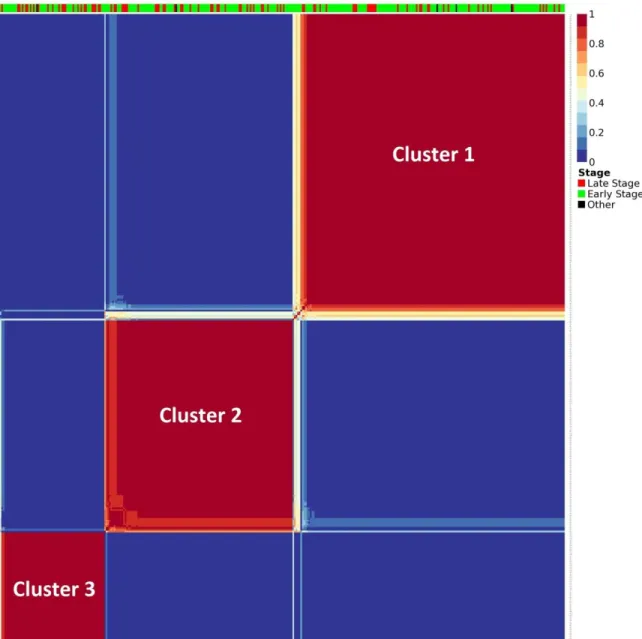
Figure 1: Histological classification of breast cancer subtypes based on architectural features and growth patterns ... 15 Figure 2: Molecular classification of breast cancer ... 19 Figure 3: Distribution of total mutational scores for the top 10 variant genes. ... 23 Figure 4: C-scores of 358 significantly mutated genes in late-stage-enriched cluster ... 38 Figure 5: Input matrix with C-scores of the top 50 variant genes. Columns represent patients (358) and rows represent genes. ... 39 Figure 6: Coefficient matrix (H), 3x358 in size, used for assigning samples to clusters. Columns represent patients and rows represent metagenes. ... 40 Figure 7: Basis matrix (W), 854x3 in size, clustering the genes. ... 41 Figure 8: Consensus matrix, 358x358 in size and illustrating the stability of the

clustering. In ideal case, all the entries are expected to be either 0 or 1, making solid colored blocks. The bar on top indicates the clinical stage of each patient. ... 43 Figure 9: Optimal clustering achieved for number of clusters (k) selected as 2 using 910 top variant genes. Even though this case achieved the highest silhouette score, the low number of clusters makes the results biologically unexplainable. ... 45 Figure 10: Optimal clustering achieved for number of clusters (k) selected as 3 using 854 top variant genes. This case is determined to use for further analysis in the project. ... 45 Figure 11: Optimal clustering achieved for number of clusters (k) selected as 4 using 700 top variant genes. The deteriorating clustering quality is visible in consensus matrix’s heatmap plot and its silhouette score. ... 46 Figure 12: Optimal clustering achieved for number of clusters (k) selected as 5 using 930 top variant genes. The deteriorating clustering quality is visible in consensus matrix’s heatmap plot and its silhouette score. ... 46 Figure 13: Interaction network analysis of the top 25 genes showing the highest mutation load in the late-stage-enriched cluster compared to the early-stage-enriched cluster of patients. ... 61 Figure 14: ROC curves showing the relationship between TPR (sensitivity) and FPR (1-specificity) for each class. ... 64

LIST OF TABLES

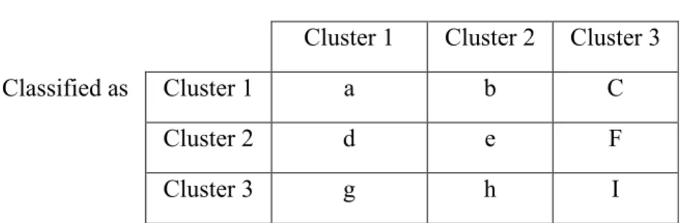
Table 1: Pseudo code for iteratively applying all potential values for k and number of features to keep ... 29 Table 2: Confusion matrix showing the number of patients predicted to be in a class and actual number of patients in that class. As an example value “a” shows the number of patients correctly predicted to be in Cluster 1. And value “b” shows the number of pa . 33 Table 3: Shows the definition of basic measures, which are used to calculate

performance measures. ... 33 Table 4: Shows the equations to be used to calculate performance measures. ... 33 Table 5: The distribution of patients to clusters according to their ER, PR and HER2 status with Fisher’s Exact test p-values ... 48 Table 6: The distribution of patients to clusters according to their age and TNBC status with Fisher’s Exact test p-values. Even though TNBC distribution resulted a significant p-value, it is not used in the project due to comparison of mutation levels of patients contradicts to biological expectation. ... 48 Table 7: The distribution of patients to clusters according to their BC stage with Fisher’s Exact test p-values. This distribution is selected to be further analyzed in the project. .. 49 Table 8: Definition early and late stage breast cancer in the project ... 49 Table 9: Distribution of patients in the clusters discovered. P-value= 0.02048 ... 50 Table 10: Significant genes that show higher mutation rates in late-stage- enriched cluster (cluster 3). ... 56 Table 11: GSEA classification of 358 genes that have significantly higher mean mutation scores in cluster 3 compared to cluster 1. Note that some of the genes in our gene list are not found in any GSEA gene family. ... 58 Table 12: Distribution of genes to functionally distinct gene families by GSEA. ... 59 Table 13: 10-fold cross-validation performance results of five classifiers. ... 63

LIST OF ABBREVIATIONS

APC Adenomatous Polyposis Coli

AUC Area Under the Curve

BC Breast Cancer

BWA Burrows-Wheeler Aligner

BWT Burrows Wheeler Transform

CADD Combined Annotation Dependent Depletion

CNV Copy Number Variation

dbSNP Single Nucleotide Polymorphism Database

DNA Deoxyribonucleic acid

DCIS Ductal Carcinoma In Situ

EM Expectation Maximization

ER Estrogen Receptor

EMT Epithelial-Mesenchymal Transition

FN False Negative

FP False Positive

GERP Genomic Evolutionary Rate Profiling

GSEA Gene Set Enrichment Analysis

HER2 Human Epidermal Growth Factor Receptor 2

IHC Immunohistochemical

IPA Ingenuity Pathway Analysis

IDC infiltrating ductal carcinoma

ICGC International Cancer Genome Consortium

INDEL Insertion / Deletion

KNN K-Nearest Neighbor

LDA Linear Discriminant Analysis

LCIS Lobular Carcinoma In Situ

ML Machine Learning

MAF Minor Allele Frequency

miRNA micro RNA

NCBI National Center for Biotechnology Information

NGS Next-Generation Sequencing

PR Progesterone Receptors

PCA Principal Component Analysis

PPV Positive Predictive Value

RF Random Forest

RNA Ribonucleic Acid

ROC Receiver Operating Characteristic

SVM Support Vector Machine

SIFT Sorts Intolerant From Tolerant

TCGA The Cancer Genome Atlas

TNBC Triple Negative Breast Cancer

TN True Negative

TNR True Negative Rate

TP True Positive

TPR True Positive Rate

UV Ultraviolet

VEP Variant Effect Predictor

WES Whole exome sequencing

Chapter 1

INTRODUCTION

Cancer is the leading cause of death worldwide accounting for 8.2 million deaths in 2012

(International Agency for Research on Cancer, 2014). According to the World Health

Organization’s latest world cancer statistics, breast cancer leads the cancers by being the most common reason for female mortality (522,000 deaths in 2012) (International

Agency for Research on Cancer, 2013). One in four cancers in women is estimated to be

a breast cancer. Moreover, since 2008, breast cancer incidents have increased by more

than 20% (International Agency for Research on Cancer, 2013).

Breast cancer is a genetically and clinically complex and heterogeneous disease,

comprised of multiple factors that are associated with distinctive histological and

biological features, clinical presentations and behaviors, and responses to therapy. Hence,

the effectiveness of a specific treatment greatly varies among patients. This multifaceted

heterogeneity poses a significant classification challenge in the identification of distinct

subtypes.

Breast cancer classification is routinely used for tailoring treatment decisions by

oncologists, and it is performed according to different schemes based on different criteria.

Major classification methods are based on histopathological analysis, grade and stage of

tumor, and analysis of gene expression signatures.

With recent advancements in next-generation sequencing (NGS) methods, the

current clinical treatment practices for breast cancer classification may benefit from the

classification may be achieved. As the genome sequencing costs are getting cheaper

using NGS technology, mutational profiles of tumor samples can be compared against

those of the normal samples from the same patients to identify somatic mutations that are

specific to a particular patient. Such information from hundreds and thousands of patients

could be effective used by computational methods to cluster them into clinically

distinguishable subgroups and eventually use this information for effective treatment of

cancer patients.

In this work we develop a novel breast cancer classification method using

machine learning methods and NGS data from whole exome sequencing of several

Chapter 2

BACKGROUND

Cancer occurs as a result of the accumulation of point mutations in critical genes,

especially those that repair damaged DNA and control cell growth and division, which

allows cells to grow and divide uncontrollably to form a tumor. Point mutations may

occur spontaneously during DNA replication or caused by mutagens that can be physical,

in the form of radiation from UV rays, X-rays or extreme heat, or chemicals such as

molecules that can change the base pairs or disrupt the structure of DNA.

There are a number of cellular processes that affect the expression level of genes

such as DNA methylation patterns in the genome, histone modifications, transcriptional

regulators some of which are transcriptional factors and miRNAs. However, majority of

these factors display a consequential effect to mutations in the DNA, while the somatic

mutations in a critical set of genes (referred to as driver genes) are considered as the

causative factors for cancers. Due to this causative effect, studying the mutational profiles

of tumor DNA is particularly attractive in the current era of personal genomics. With the

advances made in the field of genome sequencing and computational biology, it is now

possible and also cost effective to sequence only about 1.5% of the total human genome

corresponding to the protein coding regions (referred to as Exome) and yet get

information about 85% of the mutations with large effects on disease-related traits (Choi

et al., 2009).

This section will provide the background information about the basic concepts

that are used throughout the dissertation. We will explain the next-generation sequencing

variant discovery process, followed by explanation about machine learning; and a review

of available scoring methods that quantify the mutations’ impact on the gene function.

Next-Generation Sequencing (NGS)

Since NGS technology was first discovered, DNA sequencing has brought a total

revolution to our current understanding of molecular biology. Since then these

technologies have provided tremendous amounts of data, which are full of biological

insights waiting to be unraveled. Nucleotide sequencing is the name of the process for

determining the order of nucleotides in a given DNA or RNA molecule.

Sequencing has had a rapidly advancing history since its first development by

Edward Sanger in 1975. His technique relies on the chain-termination method referred to

as Sanger sequencing (Sanger, Nicklen, & Coulson, 1977). Sanger sequencing was

established as the first generation sequencing technology and is accepted as the gold

standard. The Human Genome Project was completed using this technology with a cost

of $3 billion and taking a total of 13 years.

With a demand for cheaper and faster sequencing in the early 2000s, the

sequencing field has witnessed rapid improvement with the development of

second-generation sequencing, commonly known as next-second-generation sequencing (NGS)

platforms. These platforms can produce high-throughput sequencing, processing millions

of DNA or RNA fragments from a sample, thus enabling sequencing of a complete

genome in a single day. Modern Sanger sequencing is typically performed by automated

capillary sequencing, while the high-throughput NGS technologies are all based on

majority of the NGS sequencing market and are the source of the sequencing data used in

this dissertation (Zimmerman, 2014), (DeLuca, 2013).

The most notable drawbacks of NGS when compared to earlier sequencing

techniques are higher startup costs and the cost of analyzing the generated data, which

constitutes a majority of the effort. On the other hand, NGS is not limited to analyzing

predefined regions of a genome and is not vulnerable to the inconsistent nature of

microarrays.

NGS methods can target an entire genome or only selected regions of a genome,

e.g. only coding regions of a genome which is called exome, hence named as either

whole genome sequencing (WGS) or whole exome sequencing (WES), respectively. To

summarize the overall sequencing process, small fragments of DNA or RNA are

sequenced and then either aligned to a reference genome (provided that a reference

genome exists) or fed into a de novo assembly process to build relatively contiguous

regions of the genome for further analysis.

Exome sequencing is the high-throughput sequencing of every exon in the human

genome which represents about 1% to 2% of the whole genome (depending on definition

of exome) that corresponds to about 180,000 exons from the coding region, yet contains

information on 85% of the disease-causing mutations (Choi et al., 2009). When compared

to WGS, WES has much lower costs, which makes it possible to perform a standardized

experimental procedure for patients suffering from many diseases, and then help to

discover the causative factors of the disease. However, this ability is balanced by the

calling the true variants, annotating the effects of the changes, filtering the false positive

calls, identifying plausible variants and experimental validation of results.

Variant Discovery

After the sequence reads are aligned to a reference genome, the next step is variant

discovery to identify variable sites in a tumor genome. This procedure can suffer from

high error rates that are due to several factors, including base calling step in sequencers,

alignment errors or insufficient depth of coverage. Variant discovery, often referred to as

variant calling, involves the execution of a number of computational steps in a sequential

order. The whole set of computational steps is called a variant calling pipeline, which

typically contains an aligner and a variant caller with a number of intermediate data

processing steps. As the name suggests, the aligner maps reads to a reference genome and

variant caller identifies variant sites and assigns a genotype to the subject(s).

Sequence alignment is a string matching problem and most efficient methods are

based on Burrows-Wheeler Transform (BWT), which uses data compression to gain

speed and memory efficiency. Among few other aligners, (MOSAIK (Lee et al., 2014),

and CUSHAW3 (Liu, Popp, & Schmidt, 2014)) BWT based aligners including

Burrows-Wheeler Aligner (BWA) BWA mem (H. Li, 2013), BWA sampe (H. Li & Durbin, 2009)

and Bowtie2 (Langmead & Salzberg, 2012) are the most commonly used algorithms.

According to a recent publication, making performance comparison of currently in use

aligners, BWT based aligners achieve similar results, due to their similar algorithms and

out performing other aligners (Cornish & Guda, 2015).

Unlike aligners, there are many variant callers using a variety of algorithms.

section. Main genomic variations that variant callers aim to identify include: single

nucleotide variations (SNVs), and small insertion and deletions (INDELs). Based on the

information from SNVs and INDELs, the consequent effects on transcription such as

splice junctions and splice variants, and on translation such as synonymous and

non-synonymous mutations, loss or gain of stop codons, frame shifts, etc., can be identified.

Even with well-mapped, aligned and calibrated reads resolving simple single nucleotide

variations require sensitive and specific methods and is a challenging task.

SNVs are categorized based on several criteria. Firstly, variations are

distinguished by the way they are inherited. If a variation is identified in germline cells

i.e. sperm or egg cells, it is called as germline variation, and this variation may be

inherited from a parent to an offspring. Alternatively, the genomic variations found in

somatic cells are named as somatic mutations. Somatic mutations are not inherited from a

parent, rather they are acquired by an individual during his/her life time and not passed

on to progeny. Secondly, variations that cause a change in the translated amino acid are

called non-synonymous variations, and those that do not change the amino translated

acid, are called synonymous variations. Lastly, genomic variations with less than 0.05

minor allele frequency (MAF) are considered rare variants that are associated with

diseases and hence are called as mutations.

In this work, we focus on the somatic non-synonymous mutations that occur in

Machine Learning and Data Mining

Machine learning (ML) and data mining are research areas in computer science, where

these names often used interchangeably. ML has gained high attention in recent years due

to the availability of high-throughput data from biological experiments with parallel

advances in the computing power to process and analyze the data using sophisticated

computational tools.

Machine learning is defined as a computational method, aimed to build models,

identify patterns and other regularities in data, and using the experience received from

past information or previous runs available to the learner to improve its performance. The

origin of machine learning dates back to 1957, when the perception model invented based

on the human brain neurons. On the other hand, data mining is a much younger field, first appeared in early 1990s in the database community, which is closely related to and using

techniques from machine learning. Data mining aims to extract useful information from a

data set and transform it into a desirable structure for further use. Machine learning is

widely used in our daily life, example applications include filtering spam emails, weather

forecasting and streaming media suggestions based on earlier seen videos, etc.

Some major problems studied in machine learning and data mining that are used

in this work include:

Classification: The task of assigning a class for a sample. The number of classes is often small and increasing the number of classes increases the complexity of the task, but it

even can be unbound in cases such as text classification or speech recognition

Clustering: Partitioning the samples into homogeneous groups, in such a way that samples in a group are more similar in a specified measure to each other than to those in

the other groups.

Feature selection: The process of selecting a subset of relevant features to use in model building.

Machine learning algorithms can be separated in two distinct groups, namely

supervised, and unsupervised learning methods.

Supervised learning algorithms use labeled data (where each instance of the data

has a known class) to build models and use these models to predict labels of new unseen

data points. In case of continuous labels (such as temperature value in weather

forecasting) the machine learning task is named as regression and for nominal labels

(such as prediction of it will rain or not) the task is called as classification. A simple

classification example would be the prediction of whether or not it will rain today, using

historical values of temperature, humidity and wind speed, which constitute features, and

the labels are “rain” or “no rain”. In this work, we used supervised machine learning

techniques with an aim to make class prediction for breast cancer patients using mutation

profiles. There are many supervised machine learning algorithms available including:

decision trees, artificial neural networks, and support vector machines (Wagner, 2014).

Unsupervised machine learning approaches address the problem of discovering

structure in unlabeled datasets, i.e., the instances of data lack class labels. This problem is

commonly referred as cluster analysis or clustering. As a simple example, unsupervised

clustering of genes based on expression levels to identify co-regulated pathways can be

terms of genomic mutation profiles. Hierarchical clustering and k-means clustering are

the most widely used unsupervised machine learning techniques; however in the

particular case of this dissertation those methods are not sufficient to overcome

sparseness issue. For a detailed explanation of this issue, please refer to the methods

section.

Review of Variation Scoring Methods

The main significance of this work, as mentioned earlier, is to solely use somatic

mutations for breast cancer classification purpose. To achieve this goal, first we need to

convert the text-based somatic mutation data into a meaningful score, which can be used

for further computation in machine-learning. Quantifying the effect of genomic mutations

by itself is a complicated task and there are several methods available for this task. Here,

we present a brief survey of the widely used recent methods. For a detailed review, please

refer to Ritchie and Flicek, 2014 (Ritchie & Flicek, 2014).

Modern sequencing methods yield an extensive list of sequence variations, which

makes manual investigation infeasible; therefore, we need algorithms that can predict the

effect of the discovered genomic variations. These methods can be categorized according

to the underlying algorithm strategy. Firstly, there are several methods using annotations

based on overlap with and proximity to functional elements. These tools consider

annotations of regulatory elements, including regions of open chromatin, regions marked

by histone modification and sequences bound by specific transcription factors. Secondly,

biologically informed rule-based annotation methods use the knowledge of relatively

better understood functions of particular nucleotide sequences and make allele-specific

analysis which include the Ensembl Variant Effect Predictor (VEP) (McLaren et al.,

2010), ANNOVAR (K. Wang, Li, & Hakonarson, 2010), and SnpEff (Cingolani et al.,

2012). Thirdly, we can group methods using annotations based on sequence motifs and

constraints estimated from multiple sequence alignments. These methods evaluate the

variations using their genomic position and employ the fact that if a variation is

discovered in the proximity of a frequently appearing motif or evolutionary conserved

region, then it is expected to impart a higher impact on protein function. Examples

include the widely used the Genomic Evolutionary Rate Profiling (GERP) (Cooper et al.,

2005) and Sorts Intolerant From Tolerant (SIFT) (Ng & Henikoff, 2001) algorithms.

Finally, integrative approaches, using supervised learning algorithms, employ an

alternative approach by attempting to learn informative annotations or combinations of

annotations, by comparing known functional variants with variants for which there is no

direct evidence of functional consequences. The main idea here is to use a ‘training set’

of variants that are labeled as ‘damaging’ or ‘benign’ to identify features or combination of features, which can be used to discriminate between two classes and make accurate

predictions for unseen variants. This approach has been adopted by several tools such as

PolyPhen (Adzhubei et al., 2010) and MutationTaster (Schwarz, Rödelsperger, Schuelke,

& Seelow, 2010).

In this work, we used a more recent method named as Combined Annotation

Dependent Depletion (CADD) (Kircher et al., 2014), which incorporates both genic and

regulatory annotations, as described in the last category above. In contrast to other tools

in its category, CADD uses a training set of variants that have become fixed in the human

that are not observed in human populations. Hence, CADD uses a much larger training

set and avoids sampling (ascertainment) biases associated with existing databases of

Chapter 3

LITERATURE REVIEW

Breast Cancer Staging

The most basic and widely used approach in evaluating treatment options for breast

cancer patients involves determining the clinical stage. The stage of breast cancer

explains the extent of the cancer in the body and determined based on mainly three

measures including tumor size, lymph node status and incidence of metastatic growth.

Stage I tumors are measured up to two centimeters and no lymph node involvement have

been observed. These tumors often called in-situ carcinomas and regarded as a better

prognosis group. Stage II tumors are considered to be between two to five centimeters, or

have spread to the lymph nodes under the arm on the same side as the initiating breast.

Like Stage I tumors, Stage II tumors are also generally effectively treatable. Stage III

tumors are more than two inches in diameter and lymph nodes are heavily involved, or

cancer has spread to other lymph nodes or tissues near the initiating breast. And lastly,

Stage IV tumors are noted with a metastasis that has been identified on underarm,

internal mammary lymph nodes or other organs of the body ("Breast cancer stages",

retrieved from http://www.cancercenter.com/breast-cancer/stages/,”, “Breast Cancer

Stages", retrieved from http://www.nationalbreastcancer.org/breast-cancer-stages,”,

“Breast Cancer Staging and Stages", retrieved from http://ww5.komen.org/BreastCancer/StagingofBreastCancer.html,”).

Current Breast Cancer Classification

The classification of breast cancer currently involves the evaluation of histological

criteria based on morphology and immunohistochemical (IHC) analyses. The traditional

parameters such as histological type, tumor size, histological grade and axillary

lymph-node involvement have been shown to correlate with clinical outcome and provide the

basis for prognostic evaluation (Elston, Ellis, & Pinder, 1999). In addition, IHC markers

such as the expression of hormone receptors (estrogen (ER) and progesterone receptors

(PR)) and the overexpression and/or amplification of the human epidermal growth factor receptor 2 (HER2) provide additional therapeutic predictive value and have important

role in the treatment decision (Harris et al., 2007). As a more modern approach,

microarray-based expression analysis of a select gene panel provides a comprehensive

molecular taxonomic classification to breast cancer tumors. This approach has emerged

as a standard to identify clinically distinguishable molecular subtypes for use in the

current clinical practice.

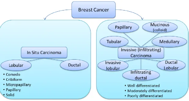
Histopathological Classification

From histopathological perspective, breast cancer can be broadly categorized into in situ

carcinoma and invasive (infiltrating) carcinoma. Breast carcinoma in situ is further

categorized into two types as ductal carcinoma in situ (DCIS) and lobular carcinoma in

situ (LCIS), based on growth patterns and cytological features. DCIS is seen significantly

more common than LCIS and includes a heterogeneous group of tumors. Moreover,

DCIS tumors have traditionally been categorized into five well recognized subtypes

based on their architectural features namely Comedo, Cribiform, Micropapillary,

group of tumors and is sub-classified into several histological subtypes namely

infiltrating ductal, invasive lobular, ductal/lobular, mucinous (colloid), tubular, medullary

and papillary carcinomas. From these subtypes the most common is infiltrating ductal

carcinoma (IDC), which covers 70-80% of all invasive carcinomas (C. I. Li, Uribe, &

Daling, 2005). Further, IDC is also sub-classified according to tumor grade, which is

assessed by evaluating the nuclear pleomorphism, glandular/tubule formation and

proliferative activity (mitotic index). Three main IDC sub-classes by grade are namely

well-differentiated (grade 1), moderately differentiated (grade 2) or poorly differentiated

(grade 3) (Lester & Bose, 2009). This classification is done based on three main criteria

namely, nuclear pleomorphism, glandular/tubule formation and mitotic rate.

Figure 1: Histological classification of breast cancer subtypes based on architectural features and growth patterns. (Malhotra, Zhao, Band, & Band, 2010)

ER, PR and HER2

In conjunction with histopathological classification, characterization of breast cancers

based on the expression of strong biomarkers such as ER, PR, and HER2 has a key role

in guiding therapeutic decisions. About 75-80% of all breast cancers are hormone

receptor positive, and standardized IHC assays are used to determine the selection of

patients for hormone-based therapies. In addition, HER2, an oncogene, is the only

predictive marker checked routinely for clinical purpose. Even though there is an inverse

association between hormone receptors and HER2, 10-15% of all breast cancers are both

hormone receptor and HER2 positive, which are considered to be selected for anti-HER2

based therapies such as the humanized monoclonal HER2 antibody, trastuzumab, which

targets the extracellular domain of the HER2 receptor (Konecny et al., 2003). Lastly, the

10-15% of breast cancer patients are recognized by being both hormone receptor

(ER&PR) negative and HER2 negative, which are known as triple negative breast

cancers (TNBCs). Unfortunately, this type of the breast cancer has the worst prognosis

and currently there is not an effective treatment option for TNBCs (Dawson, Provenzano,

& Caldas, 2009).

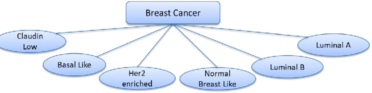
Molecular Classification of Breast Cancers

As a more recent technology, gene expression analysis based on microarray studies gave

researchers an opportunity to begin moving towards comprehensive molecular profiling

of breast cancer tumors. These studies have led to the discovery of clinically relevant

molecular breast cancer subtypes and provided additional insights about the heterogeneity

of the disease (Hu et al., 2006; Perou, Sørlie, & Eisen, 2000; Sørlie & Perou, 2001).

identification of five distinct breast cancer subtypes (Figure 2) namely Luminal A,

Luminal B, HER2 overexpressing, Basal-like and Normal breast tissue-like. Importantly,

this molecular classification has successfully discovered sub-classes of ER-positive

and/or PR-positive breast cancers as Luminal A and Luminal B. This is a significant

achievement because even though clinical assessment of IHC utilizes ER, PR, and HER2

status, these markers could not let the separation of these two distinct subtypes, which

have very different clinical outcomes (Sørlie & Perou, 2001; Sørlie & Tibshirani, 2003).

The differences in gene expression patterns in these subtypes reflect the basic

alterations in the cell biology of the tumor and are associated with significant variation in

clinical outcome such as overall survival and disease free survival (Sørlie & Tibshirani,

2003). Particularly, Luminal A subtype patients are found to have relatively better

prognosis while basal-like subtype patients having the worst prognosis.

Following the identification of these intrinsic subtypes, further classification of

breast cancers has been proposed. For example, a study conducted on ER-negative

tumors has revealed that basal breast cancers are actually a heterogeneous group with at

least four main subtypes, and an immune response gene expression module has been

discovered, which points to a good prognosis subtype in ER-negative breast cancer

(Teschendorff, Miremadi, Pinder, Ellis, & Caldas, 2007). Likewise, a different study has

found a new breast cancer intrinsic subtype recognized as Claudin-low or

mesenchymal-like (Prat et al., 2010). A characteristic of this subtype is to show an intermediate

prognosis between basal and luminal subtypes and to be enriched with cells showing

potential (Bruna et al., 2012; Hennessy & Gonzalez-Angulo, 2009; Lehmann et al., 2011;

Lim et al., 2009).

At first, the high cost of gene expression analysis of an abundant number of genes

was the obvious obstacle in adoption of the method for clinical purposes. To overcome

this, researchers narrowed down the gene list by finding distinct gene signatures for

breast cancer subtypes. In one study, investigators have successfully discovered 50 gene

signatures, named as PAM50 (Parker et al., 2009; Tibshirani, Hastie, Narasimhan, &

Chu, 2002), which can effectively differentiate the molecular subtypes using quantitative

real time PCR (qRT-PCR) and is accepted as a replacement for full microarray analysis

with the purpose of molecular classification of breast cancers. Moreover, it is

demonstrated that using the PAM50 gene set for molecular classification had

significantly improved the prediction accuracy for risk of relapse on ER-positive/node

negative patients compared to the model that utilizes only clinical variables such as tumor

size, axillary lymph-node status and histologic grade.

Besides the identification of intrinsic subtypes, gene expression profiling has also

been employed in discovery of distinct prognostic signatures by several groups (Paik,

Shak, Tang, & Kim, 2004; Veer, Dai, & Vijver, 2002; Vijver & He, 2002). Mammaprint,

which is a microarray-based assay of the Amsterdam 70-gene breast cancer signature,

and OncotypeDX, which is a PCR-based assay of a panel of 21 genes, have been

Figure 2: Molecular classification of breast cancer (Malhotra et al., 2010)

Other Hybrid Classification Methods

More recently, thanks to the ease of accessing breast cancer data through projects such as

TCGA and organizations like International Cancer Genome Consortium (ICGC), several

methods proposing integration of multiple approaches for breast cancer clustering have

been published. In 2012, Curtis et al. demonstrated a method combining genome and

transcriptome assessments of 2,000 breast cancer patients. By examining the impact of

somatic copy number aberrations on the transcriptome, they suggested a novel molecular

stratification of breast cancer and revealed novel subgroups (Curtis et al., 2012).

Likewise, in 2014, Ali et al. classified breasts cancer into 10 subtypes based on the

integration of genomic (copy number variation) and transcriptomic (gene expression)

data (Ali et al., 2014). Also in another study, researchers have shown a computational

method that combines gene expression and DNA methylation data to implement machine

learning aided breast cancer patient classification (List et al., 2014). Lastly, in a recent

publication, researchers have proposed a network-based stratification of tumor mutations

interaction networks and applied non-negative matrix factorization to form four subtypes

Chapter 4

MATERIALS AND METHODS

Datasets

In development of this project, we downloaded the sequence variation data in variant call

format (vcf) for the TCGA breast cancer whole exome sequencing data. Since the data in

TCGA comes from a diverse group of patients, to eliminate the population heterogeneity

effect, we retrieved a subset of breast cancer patients (n=358) by selecting only white, not

Hispanic or Latino patients whose clinical and whole exome sequence data are available.

The sequencing data presented in TCGA is processed using several variant callers

including, VarScan2 (Koboldt et al., 2012), SomaticSniper (Larson et al., 2012) Samtools

(H. Li, Ruan, & Durbin, 2008) . Based on our previous experience with variant callers

and supporting literature (Q. Wang et al., 2013), we used the variants discovered by

VarScan2. We obtained an average of 17,640 point variations per patient, generated by

VarScan2, a highly sensitive tool to detection of somatic mutations in exome sequencing

data from normal-tumor pairs.

Data Representation

In this study we used CADD, a method that integrates functional annotations,

conservation, and gene-model information into a single score called C-score. As

mentioned in the original publication, (Kircher et al., 2014) C-scores correlate with

allelic diversity, annotations of functionality, pathogenicity, disease severity,

experimentally measured regulatory effects, and complex trait associations. This score is

denotes more deleterious effects; however since our clustering (NMF) algorithm requires

all data entries to be positive, we transformed all the scores by adding the minimum score

to the original scores.

Our method uses an extensive data structure (mutation score matrix) to keep track

of all the deleteriousness scores (C-scores) of somatic mutations used for machine

learning. The mutation score matrix represents a table that contains the genes in rows and

the patients in columns, yielding a matrix of size 18,117 rows by 358 columns, with at

least one mutation in each row. And each cell contains the sum of all C-scores of

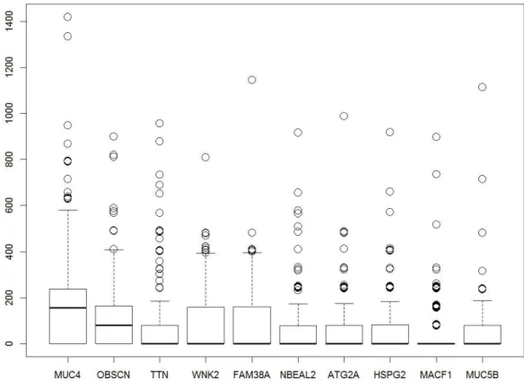
mutations found in a gene for a patient. C-scores in the mutation score matrix ranges

from 0 to 1417.14 and distribution of scores for top 10 variant genes can be seen in

Figure 3. (The Python codes developed to build the data structure and apply

preprocessing steps are provided in the Appendix.) Comparison against the COSMIC

database shows that nine out of these 10 genes (with the exception of FAM38A gene)

have evidence of abundant accumulation of somatic mutations in large population screens

Figure 3: Distribution of total mutational scores for the top 10 variant genes.

Somatic mutation profiles of BC patients exhibit a very sparse data form, unlike

other data types such as gene expression or methylation in which nearly all genes or

markers are assigned a quantitative value in all the patients. Even clinically identical patients may share no more than a single mutation (Bell et al., 2011; Lawrence et al.,

2013; TCGA, 2012). Therefore, this problem introduces too many zero valued entries to

the main data structure (96%). On the other hand, from machine learning perspective,

having a limited number of patients (a far less number of patients than the number of

effected genes in the cohort) introduces a dimensionality challenge commonly known as

the “curse of dimensionality” in machine learning. Generally machine learning algorithms desire to use a dataset, which has number of cases at least 10 times the

number of features, hence giving a minimum 10:1 sample-to-feature ratio. However, in

this study we are faced with a challenge as we observed the sample-to-feature ratio of

1:50 (358/18117) in the main data structure.

In order to overcome the aforementioned challenges, generally there are two

popular approaches, namely; feature extraction and feature selection. Feature extraction

transforms the current existing features into a lower dimensional space and widely used

example methods include principal component analysis (PCA) and linear discriminant

analysis (LDA), while feature selection selects a subset of features without applying any

transformation. These methods increase the sample-to-feature ratio and decrease the

sparseness hence making the clustering both feasible and more effective. In this

dissertation we used both feature selection and feature extraction in succession, as further

explained in below.

Clustering

We implemented an 𝑚 × 𝑛 mutation score matrix to keep track of the sum of the variant scores in all genes, where m is the number of genes (18,117) and n is the number of

samples (358 patients). The value in entry (i, j) indicates the mutation score of gene i in

sample j, which is the sum of all C-scores of mutations found in the gene i for the sample

j.

We used NMF method for clustering, which aims to find a small number of

metagenes, each defined as a positive linear combination of all the genes so that the

method can approximate the mutation load of the samples as positive linear combinations

of these metagenes. Mathematically, this corresponds to factoring a given non-negative

entries, 𝐴 ≈ 𝑊𝐻 using a positive integer number 𝑘 < 𝑚𝑖𝑛{𝑚, 𝑛}. Matrix W, called as a basis matrix and has size 𝑚 × 𝑘, with each of the k columns defining a metagene; and entry 𝑤_𝑖𝑗 represents the coefficient of gene 𝑖 in metagene 𝑗. Matrix H is named as coefficient matrix and has size 𝑘𝑥𝑛, with each of the m columns representing the metagene expression pattern of the corresponding sample; and entry ℎ_𝑖𝑗 represents the mutation load of metagene 𝑖 in sample 𝑗. There are multiple solutions to this problem and in this study we adopt a method by Brunet et al. (Brunet, Tamayo, Golub, & Mesirov,

2004) that was shown to perform better. The solution to form factors W and H can be

obtained as explained in the following. The method starts by randomly initializing the

matrices W and H and iteratively updates W and H to minimize a divergence function. W

and H are updated by using the coupled divergence equations shown in Equation 1.

𝑊_𝑖𝑎 ← 𝑊_𝑖𝑎∑ 𝐻𝑢 𝑎𝑢𝐴𝑖𝑢⁄(𝑊𝐻)𝑖𝑢

∑ 𝐻𝑣 𝑎𝑣 , 𝐻𝑎𝑢 ← 𝐻𝑎𝑢

∑ 𝑊𝑖 𝑖𝑎𝐴𝑖𝑢⁄(𝑊𝐻)𝑖𝑢

∑ 𝑊𝑘 𝑘𝑎

Equation 1: Coupled divergence equations to update the W and H matrices

As a result of factorization, we use coefficient matrix H to group our samples into

given number (𝑘) of clusters. Algorithm assigns each sample according to the highest scored metagene in patients designated column in matrix H; meaning that sample 𝑗 will be assigned to the cluster 𝑖 if ℎ_𝑖𝑗 is the highest entry in column 𝑗.

To specify the optimal number of clusters (rank of clustering) and features (genes)

to use in clustering, we used consensus matrix and average silhouette width of consensus

Since the NMF algorithm starts with a random initial class assignment of samples,

repeated runs over the same sample set with constant input parameters may not result in

the same sample assigned to the same class between the runs; however, if we observe

only a little variation in these associations between runs, then we can conclude with

confidence that a strong clustering was performed for this set of parameters (number of

clusters and features). This idea forms the basis for our clustering performance

evaluations.

Clustering Quality Assessment Methods: Consensus Matrix

Consensus matrix is a concept proposed by Brunet et al. (Brunet et al., 2004) providing

visual insights about the performance of clustering. The concept can be explained as

follows. In each run, sample to class assignments can be represented by a connectivity

matrix 𝐶 of size 𝑚𝑥𝑚 by entering 𝑐_𝑖𝑗 = 1 if samples 𝑖 and 𝑗 are assigned to the same cluster and 𝑐_𝑖𝑗 = 0 otherwise. Then the consensus matrix, 𝐶̅, can be calculated by averaging the connectivity matrix 𝐶 for many clustering runs. (We selected to use 100) The value in 𝐶̅_𝑖𝑗 ranges from 0 to 1 and reflects the probability of samples 𝑖 and 𝑗 assigned to the same cluster. In the case of a stable clustering then we expect to see most

of the values in 𝐶̅ to be close to 0 or 1.

Clustering Quality Assessment Methods: Silhouette Score

In addition to the consensus matrix, we used average silhouette width of consensus

matrix (silhouette(consensus)), introduced by Rousseeuw (Rousseeuw, 1987), to

quantitatively measure the stability of the clustering runs with different parameters.

average dissimilarity/distance of sample 𝑖 with all other data within its cluster, the value of 𝑎(𝑖) will then indicate how well the sample 𝑖 fits into its assigned cluster by having a smaller value showing better assignment. Then we can define 𝑏(𝑖) by the lowest average dissimilarity of sample 𝑖 to any other cluster that 𝑖 is not a member. In other words 𝑏(𝑖) indicates the average dissimilarity of sample 𝑖 to its closest neighboring cluster or its next best fit cluster. Then the silhouette score of a sample can be calculated as in Equation 2

below. The value of 𝑠(𝑖) can range from -1 to 1, and being close to 1 means that the sample is perfectly clustered. And average of 𝑠(𝑖) over all the samples, named as average silhouette width, shows how well the data has been clustered.

𝑠(𝑖) = { 1 −𝑎(𝑖)_𝑏(𝑖), if 𝑎(𝑖) < 𝑏(𝑖) 0, if 𝑎(𝑖) = 𝑏(𝑖) 𝑏(𝑖) 𝑎(𝑖)− 1, if 𝑎(𝑖) > 𝑏(𝑖)

{𝑎(𝑖),𝑏(𝑖)}

Equation 2: Equation shows how the silhouette score of sample can be computed

Lastly, among several implementations of NMF in various programming

languages, we selected to use an R implementation of NMF, published by Gaujoux and

Seoighe (Gaujoux & Seoighe, 2010), because of its efficient and flexible parallel

processing design and ease of applicability to our study. (The R script preparing the data

and running NMF algorithm is provided in the Appendix.)

Feature Selection and Optimization of Clustering

As also mentioned earlier feature selection constitutes an essential step in any machine

learning algorithms. We separately performed feature selection for supervised

Due to the higher number of features (tens of thousands genes) being much more

than the number of samples (hundreds of samples), we first used feature selection to

select only the informative features for clustering; thus to reduce the feature size. We

ranked the features in decreasing order of their variance values (Equation 3) and selected

top n features for clustering.

𝑆2 ₌∑(𝑋 − 𝑋̅)2

𝑛 − 1

Equation 3: Variance formula

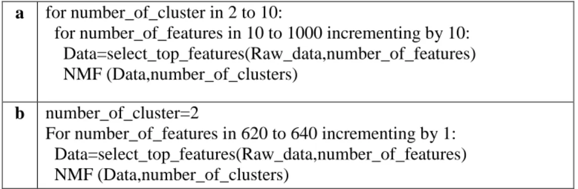
To find the most accurate clustering case, we iteratively run the clustering

algorithm over a range of biologically reasonable parameters which is form 2 to 5 clusters

and for selected top 10 to 1000 variant genes. Since running the algorithm for each

number of cluster and for each 1000 genes would be computationally intensive and not

necessary, in finding the correct number of genes we firstly run the algorithm for genes

that increase 10 each time (10 genes, 20 genes etc.). And in the second step; we run the

algorithm with all the genes in the range around the point we received the highest

consensus silhouette score. As an real case example; we receive the highest silhouette

score for 850 genes with 3 clusters, in the second step we run the algorithm for all the

genes from 840 to 860 genes and found that 856 is actually producing the best clustering.

For better and easier understanding, we present this algorithm in the pseudo code below

in Table. 1. In finding of Later we used the consensus matrix’s silhouette score to

a for number_of_cluster in 2 to 10:

for number_of_features in 10 to 1000 incrementing by 10: Data=select_top_features(Raw_data,number_of_features) NMF (Data,number_of_clusters)

b number_of_cluster=2

For number_of_features in 620 to 640 incrementing by 1: Data=select_top_features(Raw_data,number_of_features) NMF (Data,number_of_clusters)

Table 1: Pseudo code for iteratively applying all potential values for k and number of features to keep

Characterization of Clusters

To characterize the clusters we discovered, we correlated the samples in the clusters with

their clinical features. For simplicity, we defined stage I and II as early stage and stage III

and IV as late stage. The Fisher’s exact test was used to assess the stage tendency of

clusters.

We compared the mutation score of genes between clusters using the Wilcoxon

rank-sum test, and adjusted the multiple testing with the false discovery rate (FDR). The

FDR was estimated using the Benjamini-Hochberg procedure (Benjamini & Hochberg,

1995). We used the R language and environment (RDevelopment, 2012) to run all the

statistical tests. In addition, we performed functional analysis of the differentially

mutated genes between the clusters using the Ingenuity Pathway Analysis (“IPA;

Ingenuity Systems Inc.; Redwood, CA, USA,” n.d.) and the Gene Set Enrichment Analysis (GSEA) tools (Subramanian, Tamayo, Mootha, Mukherjee, & Ebert, 2005).

Development of Supervised Classification Model

For running feature selection, classification model generation using ML algorithms and

performance measurements, we used the Waikato Environment for Knowledge Analysis

(WEKA) (Hall et al., 2009) framework, which is an open-source, Java-based framework.

For feature selection, we used the Information gain attribute evaluator (Mitchell,

1997), and Ranker algorithms implemented in Weka for evaluation and searching of the

features. We used five diverse and most popular ML algorithms; namely RF (Breiman,

2001), Naïve Bayes (Rish, 2001), C4.5 (named as J48 in Weka) (Salzberg, 1994), SVM

(Platt, 1998), and KNN (Stevens, Cover, & Hart, 1967) to build classification models.

For performance measurements, we used 10-fold validation. In 10-fold

cross-validation, patients are randomly partitioned into ten equal sized parts keeping the class

ratio const1ant in each part; nine parts are used for training the classifiers and remaining

part is used for testing. This procedure is repeated ten times, resulting each part is tested

against the models built using other nine parts. The average of performance

measurements of all ten iterations is considered as an unbiased estimate of the whole

classification model. We report the performance of the classifiers using standard

classification evaluation metrics, including: accuracy, sensitivity (true positive rate, TPR,

also called recall), specificity (true negative rate, TNR), false positive rate, false negative

rate, precision (Positive Predictive Value, PPV) and F measure (also called F1 score). In

Table 2, we show confusion matrix, also called contingency table, which is used to

calculate performance measures, and Table 3 values making true positives (TP), false

positives (FP), true negative (TN), and false negatives (FN), are shown And the equations

ROC curves, which graphically present the performance of classifiers for each class and

calculate the area under the curve (AUC) as a numeric evaluation of ROC curves. Also,

we would like to note that even though most of these measures initially defined for binary

classification (having only two classes); they are applicable to multiclass classification by

(Sensitivity) TPR: TP/(TP+FN) (Specificity)TNR: TN/(TN+FP) FPR: FP/(FP+TN) or 1- FNR: FN/(FN+TP) (Precision) PPV: TP/(TP+FP) F measure: 2*(PPV*TPR)/(PPV+TPR)

Table 4: Shows the equations to be used to calculate performance measures. Actual label

Cluster 1 Cluster 2 Cluster 3

Classified as Cluster 1 a b C

Cluster 2 d e F

Cluster 3 g h I

Table 2: Confusion matrix showing the number of patients predicted to be in a class and actual number of patients in that class. As an example value “a” shows the number of patients correctly predicted to be in Cluster 1. And value “b” shows the number of pa Cluster 1 Cluster 2 Cluster 3 TP: a e i FP: b+c e+f h+i

TN: e+f+h+i d+g+f+i d+e+g+h

FN: d+g e+h f+i

Table 3: Shows the definition of basic measures, which are used to calculate performance measures.

Permutation Test

Finally, to validate the strength of the achieved prediction accuracy, we run a permutation

test. For this test we generated 10,000 datasets by randomly shuffling patient labels in our

dataset, while keeping the number of patients in each class constant. We run 10-fold

cross-validation with RF classification algorithm together with feature selection step on

these datasets, in the same way used for the real data in the study. We calculated a

p-value by the number of times this validation produced a better accuracy on randomly

shuffled dataset divided by 10,000 as seen in Equation 4.

𝑃𝑒𝑟𝑚𝑢𝑡𝑎𝑡𝑖𝑜𝑛 𝑡𝑒𝑠𝑡 𝑃 − 𝑣𝑎𝑙𝑢𝑒 =#(𝐴𝑐𝑐𝑢𝑟𝑎𝑐𝑦𝑟𝑎𝑛𝑑𝑜𝑚> 𝐴𝑐𝑐𝑢𝑟𝑎𝑐𝑦𝑜𝑟𝑖𝑔𝑖𝑛𝑎𝑙)

10000

Chapter 5

RESULTS AND DISCUSSION

Exome Data Analysis and Variant Calling

We have obtained an average of 17,640 point variations per patient generated by

VarScan2 (Koboldt et al., 2012) and applied a set of filters to select only those that are

likely to exhibit an impact on the function and/or the structure of the gene or protein.

Since the generation of next-generation sequencing (NGS) data and variant calling

involves several error prone steps, filtration of the variant data constitutes a major step in

variant analysis. Firstly, we focus only on the somatic (non-inherited) and

nonsynonymous (cause a change in the translated amino acid) point mutations because of

their perceived impact on disease initiation and progression. Secondly, even though

exome sequencing targets only the coding regions of DNA, the exome capture kits often

amplify off-target non-coding regions such as intergenic, untranslated and intron regions.

Hence, we filter out all the variations outside of the coding region. We analyze the

remaining variations by their impact on the function or structure of the resulting protein.

Finally, we check the population frequency of remaining variations in Single Nucleotide

Polymorphism Database (dbSNP) (Sherry et al., 2001), which is a public achieve for

genetic variation developed and hosted by National Center for Biotechnology

Information (NCBI). In this step, we filter out the variations that are commonly found in

population and hence are not necessarily associated with a disease. Generally, variations

with less than 0.05 minor allele frequency (MAF) are considered as phenotype-causing

Classification of Breast Cancers Based On Somatic Mutations

As a prior step before clustering, we applied feature selection by ranking the features

(genes) in decreasing order of their variance value and selected top n features for

clustering. We optimized the size of n to be 854 genes in our clustering method and

determined the number of clusters k as explained in “Feature selection and optimization

of clustering” section to be 3. Later using the NMF clustering algorithm on our dataset, we stably clustered the samples into 3 groups using the top 854 genes, which have the

highest variance values of mutation scores across all the samples. The three groups

Cluster 1, 2, and 3 involve 169, 121 and 68 patients, respectively. Refer to Materials and

Methods section for more details about the NMF method and to Optimization results

section for detailed information on results of the optimization steps.

Unsupervised clustering is the task of grouping a set of samples that have no label

information, which results in grouping samples in such a way that samples in the same

group are more similar in a specified measure to each other than to those in the other

groups. There are several methods trying to achieve this goal such as k-means clustering,

hierarchical clustering and expectation maximization (EM) algorithms. However, these

methods perform poorly or can not come to a solution when applied to sparse data, as is

the case in our study. Therefore, we selected to use NMF because of its proven superior

performance when tested on applications that use biological data. (Kim, Seo, Joung, &

Kim, 2011; Lawrence et al., 2013; Zheng, Zhang, Ng, Shiu, & Huang, 2011). NMF was

introduced in its modern formulation by Lee and Seung (Lee & Seung, 2001) as a method

As a factorization method, NMF algorithm takes our mutation score matrix as the

input and decomposes it to two smaller matrices (basis matrix W and coefficient matrix

H). The output coefficient matrix (matrix H) is used to make sample cluster assignments.

Refer to methods for more details.

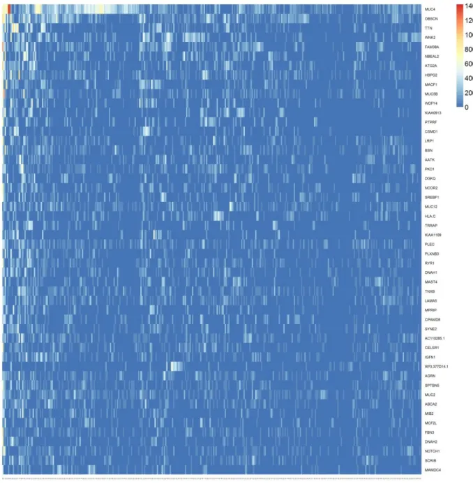
In Figure 4 we show a representation of the input data in the mutation score

matrix with statistically significant genes sorted by their variance in decreasing order;

since the data is extremely sparse the heat map consists of mostly blue cells. In order to

make the heat map more readable to human eye, we show the input data in Figure 5

focusing only the top 50 variant genes. As it can be seen, data still represents a very

sparse form (most of the cells are colored blue meaning a score of zero) that makes most

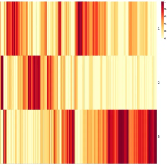
clustering approaches inapplicable. Figures 6 and 7 are the output matrices from

decomposition of the mutation score matrix, which we input to NMF algorithm. Note that

multiplication of the two output matrices will approximately yield the input data. In

Figure 7, we see the basis matrix (W), which is not used in the scope of this study;

however it could serve for clustering purpose of the genes. Figure 6 displays the

coefficient matrix (H), where the rows represent the metagenes that are a compact

representation of all the genes, and columns represent the patients. We use this matrix to

make sample to cluster associations by assigning the samples to the clusters where we

observe the highest metagene value, i.e., the dark red color (see methods section for