Variable selection using Random Forests
Robin Genuer, Jean-Michel Poggi, Christine Tuleau-Malot
To cite this version:
Robin Genuer, Jean-Michel Poggi, Christine Tuleau-Malot. Variable selection using Random
Forests. Pattern Recognition Letters, Elsevier, 2010, 31 (14), pp.2225-2236.
<
hal-00755489
>
HAL Id: hal-00755489
https://hal.archives-ouvertes.fr/hal-00755489
Submitted on 21 Nov 2012
HAL
is a multi-disciplinary open access
archive for the deposit and dissemination of
sci-entific research documents, whether they are
pub-lished or not.
The documents may come from
teaching and research institutions in France or
abroad, or from public or private research centers.
L’archive ouverte pluridisciplinaire
HAL
, est
destin´
ee au d´
epˆ
ot et `
a la diffusion de documents
scientifiques de niveau recherche, publi´
es ou non,
´
emanant des ´
etablissements d’enseignement et de
recherche fran¸
cais ou ´
etrangers, des laboratoires
publics ou priv´
es.
Variable Selection using Random Forests
Robin Genuera, Jean-Michel Poggi∗,a,b, Christine Tuleau-Malotc
aLaboratoire de Math´ematiques, Universit´e Paris-Sud 11, B ˆat. 425, 91405 Orsay, France bUniversit´e Paris 5 Descartes, France
cLaboratoire Jean-Alexandre Dieudonn´e, Universit´e Nice Sophia-Antipolis, Parc Valrose, 06108 Nice Cedex 02, France.
Abstract
This paper proposes, focusing on random forests, the increasingly used statistical method for classification and regression problems introduced by Leo Breiman in 2001, to investigate two classical issues of variable selection. The first one is to find important variables for interpretation and the second one is more restrictive and try to design a good prediction model. The main contribution is twofold: to provide some insights about the behavior of the variable importance index based on random forests and to propose a strategy involving a ranking of explanatory variables using the random forests score of importance and a stepwise ascending variable introduction strategy.
Key words: Random Forests, Regression, Classification, Variable Importance, Variable Selection, High Dimensional Data 2010 MSC: 62G09, 62H30, 62G08
1. Introduction
This paper is primarily interested in random forests for vari-able selection. Mainly methodological the main contribution is twofold: to provide some insights about the behavior of the variable importance index based on random forests and to use it to propose a two-steps algorithm for two classical problems of variable selection starting from variable importance ranking. The first problem is to find important variables for interpretation and the second one is more restrictive and try to design a good prediction model. The general strategy involves a ranking of explanatory variables using the random forests score of impor-tance and a stepwise ascending variable introduction strategy. Let us mention that we propose an heuristic strategy which does not depend on specific model hypotheses but based on data-driven thresholds to take decisions.
Before entering into details, let us shortly present in the sequel of this introduction the three main topics addressed in this paper: random forests, variable importance and variable selection.
Random forests
Random forests (RF henceforth) is a popular and very ef-ficient algorithm, based on model aggregation ideas, for both classification and regression problems, introduced by Breiman (2001). It belongs to the family of ensemble methods, appear-ing in machine learnappear-ing at the end of nineties (see for exam-ple Dietterich (1999) and Dietterich (2000)). Let us briefly
∗Corresponding author. Tel.: (33) 1 69 15 57 44; Fax: (33) 1 69 15 72 34.
Email addresses:[email protected](Robin Genuer),
[email protected](Jean-Michel Poggi),
[email protected](Christine Tuleau-Malot)
recall the statistical framework by considering a learning set
L = {(X1,Y1), . . . ,(Xn,Yn)}made of n i.i.d. observations of a
random vector (X,Y). Vector X =(X1, ...,Xp) contains
predic-tors or explanatory variables, say X ∈ Rp, and Y ∈ Y where
Yis either a class label or a numerical response. For
classifi-cation problems, a classifier t is a mapping t :Rp → Ywhile
for regression problems, we suppose that Y = s(X)+ε with
E[ε|X]= 0 and s the so-called regression function. For more
background on statistical learning, see e.g. Hastie et al. (2001). Random forests is a model building strategy providing estima-tors of either the Bayes classifier, which is the mapping
min-imizing the classification error P(Y ,t(X)), or the regression
function.
The principle of random forests is to combine many binary decision trees built using several bootstrap samples coming from the learning sample L and choosing randomly at each node a subset of explanatory variables X. More precisely, with respect to the well-known CART model building strategy (see Breiman et al. (1984)) performing a growing step followed by a
pruning one, two differences can be noted. First, at each node,
a given number (denoted by mtry) of input variables are ran-domly chosen and the best split is calculated only within this subset. Second, no pruning step is performed so all the trees of the forest are maximal trees.
In addition to CART, bagging, another well-known related tree-based method, is to be mentioned (see Breiman (1996)).
Indeed random forests with mtry = p reduce simply to
un-pruned bagging. The associated R1 packages are respectively
randomForest(intensively used in the sequel of the paper),
rpartandipredfor CART and bagging respectively (cited
1see http://www.r-project.org/
here for the sake of completeness).
RF algorithm becomes more and more popular and appears
to be very powerful in a lot of different applications (see for
ex-ample D´ıaz-Uriarte et al. (2006) for gene expression data anal-ysis) even if it is not clearly elucidated from a mathematical point of view (see the recent paper by Biau et al. (2008) about purely random forests and B¨uhlmann et al. (2002) about bag-ging). Nevertheless, Breiman (2001) sketches an explanation of the good performance of random forests related to the good quality of each tree (at least from the bias point of view) to-gether with the small correlation among the trees of the forest, where the correlation between trees is defined as the ordinary correlation of predictions on so-called out-of-bag (OOB hence-forth) samples. The OOB sample which is the set of observa-tions which are not used for building the current tree, is used to estimate the prediction error and then to evaluate variable importance.
The R package about random forests is based on the seminal contribution of Breiman et al. (2005) and is described in Liaw
et al. (2002). In this paper, we focus on therandomForest
pro-cedure. The two main parameters are mtry, the number of input variables randomly chosen at each split and ntree, the number of trees in the forest. Some details about numerical and sensi-tivity experiments can be found in Genuer et al. (2008)).
In addition, let us mention we will concentrate on the prediction performance of RF focusing on out-of-bag (OOB) error (see Breiman (2001)). We use this kind of prediction error estimate for three reasons: the main is that we are mainly interested in comparing models instead of assessing models, the second is that it gives fair estimation compared to the usual alternative test set error even if it is considered as a little bit optimistic and the last one, is that it is a default output of the randomForestprocedure, so it is used by almost all users.
Variable importance
The quantification of the variable importance (VI henceforth) is an important issue in many applied problems complement-ing variable selection by interpretation issues. In the linear re-gression framework it is examined for example by Gr¨omping (2007), making a distinction between various variance decom-position based indicators: ”dispersion importance”, ”level im-portance” or ”theoretical imim-portance” quantifying explained variance or changes in the response for a given change of each regressor. Various ways to define and compute using R such indicators are available (see Gr¨omping (2006)).
In the random forests framework, the most widely used score of importance of a given variable is the increasing in mean of the error of a tree (MSE for regression and misclassification rate for classification) in the forest when the observed values of this variable are randomly permuted in the OOB samples (let us mention that it could be slightly negative). Often, such random forests VI is called permutation importance indices in opposition to total decrease of node impurity measures already introduced in the seminal book about CART by Breiman et al. (1984).
Even if only little investigation is available about RF variable importance, some interesting facts are collected
for classification problems when this index is based on the average loss of entropy criterion, like the Gini entropy used for growing classification trees. Let us cite two remarks. The first one is that the RF Gini importance is not fair in favor of predictor variables with many categories (see Strobl et al. (2007)) while the RF permutation importance is a more reliable indicator. So we restrict our attention to this last one. The second one is that it seems that permutation importance overestimates the variable importance of highly correlated variables and a conditional variant is proposed by Strobl et
al. (2008). Let us mention that, in this paper, we do not
diagnose such a critical phenomenon for variable selection. The recent paper by Archer et al. (2008), focusing more specifically on the VI topic is also of interest. We address two crucial questions about the variable importance behavior: the importance of a group of variables and its behavior in presence of highly correlated variables. This is the first goal of this paper.
Variable selection
Many variable selection procedures are based on the cooper-ation of variable importance for ranking and model estimcooper-ation to generate, evaluate and compare a family of models. Follow-ing Kohavi et al. (1997) and Guyon et al. (2003)), it is usual to distinguish three types of variable selection methods: ”fil-ter” for which the score of variable importance does not de-pend on a given model design method; ”wrapper” which in-clude the prediction performance in the score calculation; and finally ”embedded” which intricate more closely variable selec-tion and model estimaselec-tion.
Let us briefly mention some of them, in the classification case, which are potentially competing tools, of course the wrapper methods based on VI coming from CART, and from random forests. Then some examples of embedded methods: Poggi et al. (2006) propose a method based on CART scores and using stepwise ascending procedure with elimination step; Guyon et al. (2002) and Rakotomanonjy (2003), propose meth-ods based on SVM scores and using descending elimination. More recently, Ben Ishak et al. (2008) propose a stepwise variant while Park et al. (2007) propose a ”LARS” type strategy (see Efron et al. (2004)) for classification problems. Finally let us mention a mixed approach, see Fan et al. (2008) in regression, ascending in order to avoid to select redundant
variables or, for the case n << p, descending first using a
screening procedure to reach a classical situation n ∼ p, and
then ascending using LASSO or SCAD, see Fan et al. (2001). We propose in this paper, a two-steps procedure, the second one depends on the objective (interpretation or prediction) while the first one is common. The key point is that it is entirely based on random forests, so fully non parametric and then free from the usual linar framework.
A typical situation
Let us close this section by introducing a typical situation which can be useful to capture the main ideas of this paper.
Let us consider a high dimensional (n << p) classification
problem for which the predictor variables are associated to a pixel in an image or a 3D location in the brain like in fMRI
brain activity classification problems. In such situations, of course it is clear that there is a lot of useless variables and that there exist a lot a highly correlated groups of predictors corresponding to brain regions. We emphasize that two distinct objectives about variable selection can be identified: (1) to find important variables highly related to the response variable for interpretation purpose; (2) to find a small number of variables
sufficient for a good prediction of the response variable. Key
tools combine variable importance thresholding, variable ranking and stepwise introduction of variables. Turning back to our typical example, an example of the first kind of problem is the determination of entire regions in the brain or a full parcel in an image while an instance of the second one is to exhibit a
sufficient subset of the most discriminant variables within the
previously highlighted groups. Outline
The paper is organized as follows. After this introduction, Section 2 proposes to study the behavior of the RF variable im-portance, especially in the presence of groups of highly corre-lated explanatory variables. Section 3 investigates the two clas-sical issues of variable selection using the permutation based random forests score of importance. Section 4 examines some experimental results, by focusing mainly on high dimensional classification datasets and, in order to illustrate the general
value of the strategy it is applied to a standard (n>>p)
regres-sion dataset. Finally Section 5 opens discusregres-sion about future work.
2. Variable importance
The quantification of the variable importance (abbreviated VI) is a crucial issue not only for ranking the variables before a stepwise estimation model but also to interpret data and under-stand underlying phenomenons in many applied problems.
In this section, we examine the RF variable importance
be-havior according to three different issues. The first one deals
with the sensitivity to the sample size n and the number of vari-ables p. The second examines the sensitivity to method pa-rameters mtry and ntree. The third one deals with the variable importance in presence of groups of highly correlated variables. As a result, a good choice of parameters of RF can help to better discriminate between important and useless variables. In addition, it can increase the stability of VI scores.
To illustrate this discussion, let us examine a simulated
dataset for the case n<< p, introduced by Weston et al. (2003)
and called “toys data” in the sequel. It is an equiprobable
two-class problem, Y ∈ {−1,1}, with 6 true variables, the others
be-ing some noise. This example is interestbe-ing since it constructs two near independent groups of 3 significant variables (highly, moderately and weakly correlated with response Y) and an ad-ditional group of noise variables, uncorrelated with Y. A for-ward reference to the plots on the left side of Figure 1 allow to see the variable importance picture and to note that the im-portance of the variables 1 to 3 is much higher than the one of variables 4 to 6. More precisely, the model is defined through
the conditional distribution of the Xifor Y=y:
• for 70% of data, Xi ∼ yN(i,1) for i = 1,2,3 and Xi ∼
yN(0,1) for i=4,5,6.
• for the 30% left, Xi
∼ yN(0,1) for i = 1,2,3 and Xi
∼
yN(i−3,1) for i=4,5,6.
• the other variables are noise, Xi
∼ N(0,1) for i=7, . . . ,p.
After simulation, the obtained variables are finally standard-ized.
Let us consider the toys data and compute the variable im-portance.
Remark 2.1. Let us mention that variable importance is
com-puted conditionally to a given realization even for simulated datasets. This choice which is criticizable if the objective is to reach a good estimation of an underlying constant, is consistent with the idea of staying as close as possible to the experimental situation dealing with a given dataset. In addition, the number of permutations of the observed values in the OOB sample, used to compute the score of importance is set to the default value 1. 2.1. Sensitivity to n and p
Figure 1 illustrates the behavior of variable importance for several values of n and p. Parameters ntree and mtry are set
to their default values (ntree = 500 and mtry = √p for the
classification case). Boxplots are based on 50 runs of the RF al-gorithm and for visibility, we plot the variable importance only for a few variables.
1 2 3 4 5 6 0 0.05 0.1 0.15 0.2 importance variable n=500 p=6 1 2 3 4 5 6 7 8 910 12 14 16 0 0.02 0.04 0.06 0.08 0.1 0.12 n=500 p=200 1 2 3 4 5 6 7 8 910 12 14 16 0 0.02 0.04 0.06 0.08 0.1 0.12 n=500 p=500 1 2 3 4 5 6 0 0.05 0.1 0.15 0.2 importance variable n=100 p=6 1 2 3 4 5 6 7 8 910 12 14 16 0 0.02 0.04 0.06 n=100 p=200 1 2 3 4 5 6 7 8 910 12 14 16 0 0.02 0.04 0.06 n=100 p=500
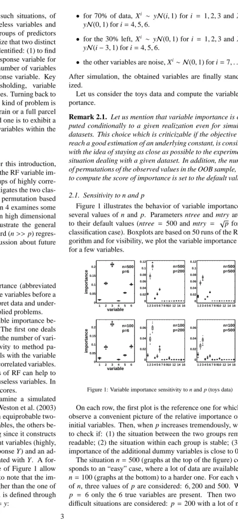
Figure 1: Variable importance sensitivity to n and p (toys data)
On each row, the first plot is the reference one for which we observe a convenient picture of the relative importance of the initial variables. Then, when p increases tremendously, we try to check if: (1) the situation between the two groups remains readable; (2) the situation within each group is stable; (3) the importance of the additional dummy variables is close to 0.
The situation n=500 (graphs at the top of the figure)
corre-sponds to an “easy” case, where a lot of data are available and
n=100 (graphs at the bottom) to a harder one. For each value
of n, three values of p are considered: 6,200 and 500. When
p = 6 only the 6 true variables are present. Then two very
difficult situations are considered: p =200 with a lot of noisy
variables and p=500 is even harder. Graphs are truncated after the 16th variable for readability (importance of noisy variables left are of the same order of magnitude as the last plotted).
Let us comment on graphs on the first row (n=500). When
p = 6 we obtain concentrated boxplots and the order is clear,
variables 2 and 6 having nearly the same importance. When
p increases, the order of magnitude of importance decreases
(note that the y-axis scale is different for p=6 and for p,6).
The order within the two groups of variables (1−3 and 4−6)
remains the same, while the overall order is modified (variable 6 is now less important than variable 2). In addition, variable importance is more unstable for huge values of p. But what is remarkable is that all noisy variables have a zero VI. So one can easily recover variables of interest.
In the second row (n = 100), we note a greater instability
since the number of observations is only moderate, but the
vari-able ranking remains quite the same. What differs is that in
the difficult situations (p=200,500) importance of some noisy
variables increases, and for example variable 4 cannot be high-lighted from noise (even variable 5 in the bottom right graph). This is due to the decreasing behavior of VI with p growing,
coming from the fact that when p = 500 the algorithm
ran-domly choose only 22 variables at each split (with the mtry default value). The probability of choosing one of the 6 true variables is really small and the less a variable is chosen, the less it can be considered as important. We will see the benefits of increasing mtry in the next paragraph.
In addition, let us remark that the variability of VI is large for true variables with respect to useless ones. This remark can be used to build some kind of test for VI (see Strobl et al. (2007)) but of course ranking is better suited for variable selection.
We now study how this VI index behaves when changing val-ues of the main method parameters.
2.2. Sensitivity to mtry and ntree
The choice of mtry and ntree can be important for the VI
computation. Let us fix n =100 and p =200. In Figure 2 we
plot variable importance obtained using three values of mtry (14 the default, 100 and 200) and two values of ntree (500 the default, and 2000). 1 2 3 4 5 6 7 8 910 12 14 16 0 0.05 0.1 0.15 0.2 importance variable ntree=500 mtry=14 1 2 3 4 5 6 7 8 910 12 14 16 0 0.05 0.1 0.15 0.2 ntree=500 mtry=100 1 2 3 4 5 6 7 8 910 12 14 16 0 0.05 0.1 0.15 0.2 ntree=500 mtry=200 1 2 3 4 5 6 7 8 910 12 14 16 0 0.05 0.1 0.15 0.2 importance variable ntree=2000 mtry=14 1 2 3 4 5 6 7 8 910 12 14 16 0 0.05 0.1 0.15 0.2 ntree=2000 mtry=100 1 2 3 4 5 6 7 8 910 12 14 16 0 0.05 0.1 0.15 0.2 ntree=2000 mtry=200
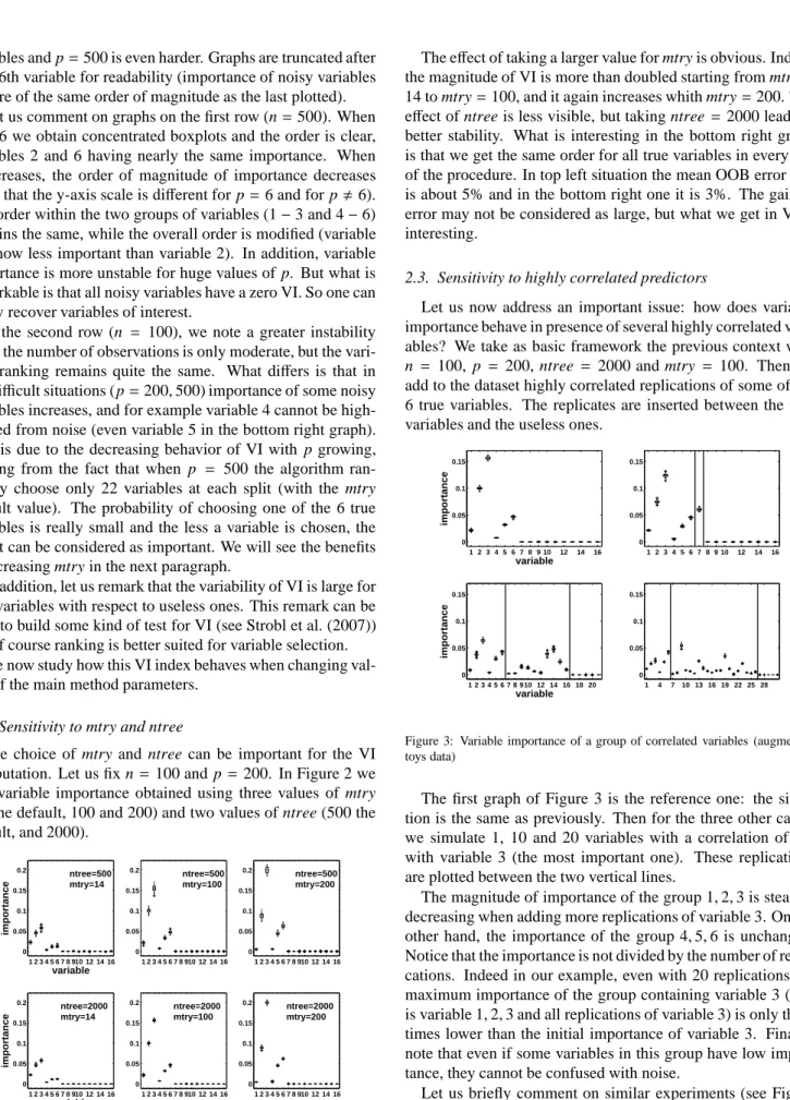
Figure 2: Variable importance sensitivity to mtry and ntree (toys data)
The effect of taking a larger value for mtry is obvious. Indeed
the magnitude of VI is more than doubled starting from mtry=
14 to mtry=100, and it again increases whith mtry=200. The
effect of ntree is less visible, but taking ntree=2000 leads to
better stability. What is interesting in the bottom right graph is that we get the same order for all true variables in every run of the procedure. In top left situation the mean OOB error rate is about 5% and in the bottom right one it is 3%. The gain in error may not be considered as large, but what we get in VI is interesting.
2.3. Sensitivity to highly correlated predictors
Let us now address an important issue: how does variable importance behave in presence of several highly correlated vari-ables? We take as basic framework the previous context with
n = 100, p = 200, ntree = 2000 and mtry = 100. Then we
add to the dataset highly correlated replications of some of the 6 true variables. The replicates are inserted between the true variables and the useless ones.
1 2 3 4 5 6 7 8 9 10 12 14 16 0 0.05 0.1 0.15 importance variable 1 2 3 4 5 6 7 8 9 10 12 14 16 0 0.05 0.1 0.15 1 2 3 4 5 6 7 8 910 12 14 16 18 20 0 0.05 0.1 0.15 importance variable 1 4 7 10 13 16 19 22 25 28 0 0.05 0.1 0.15
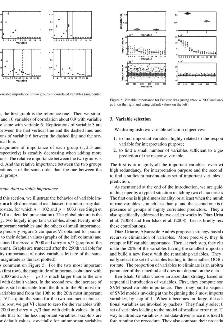
Figure 3: Variable importance of a group of correlated variables (augmented toys data)
The first graph of Figure 3 is the reference one: the situa-tion is the same as previously. Then for the three other cases,
we simulate 1, 10 and 20 variables with a correlation of 0.9
with variable 3 (the most important one). These replications are plotted between the two vertical lines.
The magnitude of importance of the group 1,2,3 is steadily
decreasing when adding more replications of variable 3. On the
other hand, the importance of the group 4,5,6 is unchanged.
Notice that the importance is not divided by the number of repli-cations. Indeed in our example, even with 20 replications the maximum importance of the group containing variable 3 (that
is variable 1,2,3 and all replications of variable 3) is only three
times lower than the initial importance of variable 3. Finally, note that even if some variables in this group have low impor-tance, they cannot be confused with noise.
Let us briefly comment on similar experiments (see Figure 4) but perturbing the basic situation not only by introducing highly correlated versions of the third variable but also of the sixth, leading to replicate the most important of each group.
1 2 3 4 5 6 7 8 9 10 12 14 16 0 0.05 0.1 0.15 importance variable 1 2 3 4 5 6 7 8 9 10 12 14 16 0 0.05 0.1 0.15 1 2 3 4 5 6 7 8 910 12 14 16 18 20 0 0.05 0.1 0.15 importance variable 1 4 7 10 13 16 19 22 25 28 0 0.05 0.1 0.15
Figure 4: Variable importance of two groups of correlated variables (augmented toys data)
Again, the first graph is the reference one. Then we
simu-late 1, 5 and 10 variables of correlation about 0.9 with variable
3 and the same with variable 6. Replications of variable 3 are plotted between the first vertical line and the dashed line, and replications of variable 6 between the dashed line and the sec-ond vertical line.
The magnitude of importance of each group (1,2,3 and
4,5,6 respectively) is steadily decreasing when adding more
replications. The relative importance between the two groups is preserved. And the relative importance between the two groups of replications is of the same order than the one between the two initial groups.
2.4. Prostate data variable importance
To end this section, we illustrate the behavior of variable im-portance on a high dimensional real dataset: the microarray data
called Prostate, for which n=102 and p=6033 (see Singh et
al. (2002) for a detailed presentation). The global picture is the following: two hugely important variables, about twenty mod-erately important variables and the others of small importance. So, more precisely Figure 5 compares VI obtained for param-eters set to their default values (graphs of the left column) and
those obtained for ntree=2000 and mtry=p/3 (graphs of the
right column). Graphs are truncated after the 250th variable for readability (importance of noisy variables left are of the same order of magnitude as the last plotted).
Let us comment on Figure 5. For the two most important variables (first row), the magnitude of importance obtained with
ntree = 2000 and mtry = p/3 is much larger than to the one obtained with default values. In the second row, the increase of magnitude is still noticeable from the third to the 9th most im-portant variables and from the 10th to the 20th most imim-portant variables, VI is quite the same for the two parameter choices. In the third row, we get VI closer to zero for the variables with
ntree =2000 and mtry= p/3 than with default values. In ad-dition, note that for the less important variables, boxplots are larger for default values, especially for unimportant variables (from the 200th to the 250th).
1 2 0 0.05 0.1 variable importance 1 2 0 0.05 0.1 3 4 5 6 7 8 9 10 12 14 16 18 20 0 5 10 15x 10 −3 importance variable 3 4 5 6 7 8 9 10 12 14 16 18 20 0 5 10 15x 10 −3 200 210 220 230 240 250 −5 0 5 10 x 10−4 importance variable 200 210 220 230 240 250 −5 0 5 10 x 10−4
Figure 5: Variable importance for Prostate data (using ntree=2000 and mtry=
p/3, on the right and using default values on the left)
3. Variable selection
We distinguish two variable selection objectives:
1. to find important variables highly related to the response variable for interpretation purpose;
2. to find a small number of variables sufficient to a good
prediction of the response variable.
The first is to magnify all the important variables, even with high redundancy, for interpretation purpose and the second is
to find a sufficient parsimonious set of important variables for
prediction.
As mentioned at the end of the introduction, we are guided in this paper by a typical situation matching two characteristics. The first one is high dimensionality, or at least when the number of true variables is much less than p, and the second one is the presence of groups of highly correlated predictors. They are also specifically addressed in two earlier works by D´ıaz-Uriarte et al. (2006) and Ben Ishak et al. (2008). Let us briefly recall these contributions.
D´ıaz-Uriarte, Alvarez de Andr´es propose a strategy based on recursive elimination of variables. More precisely, they first compute RF variable importance. Then, at each step, they elim-inate the 20% of the variables having the smallest importance and build a new forest with the remaining variables. They fi-nally select the set of variables leading to the smallest OOB er-ror rate. The proportion of variables to eliminate is an arbitrary parameter of their method and does not depend on the data.
Ben Ishak, Ghattas choose an ascendant strategy based on a sequential introduction of variables. First, they compute some SVM-based variable importance. Then, they build a sequence of SVM models invoking at the beginning the k most important variables, by step of 1. When k becomes too large, the addi-tional variables are invoked by packets. They finally select the set of variables leading to the model of smallest error rate. The way to introduce variables is not data-driven since it is fixed be-fore running the procedure. They also compare their procedure with a similar one using RF instead of SVM.
3.1. Procedure
We propose the following two-steps procedure, the first one is common while the second one depends on the objective: Step 1. Preliminary elimination and ranking:
• Compute the RF scores of importance, cancel the
variables of small importance;
• Order the m remaining variables in decreasing
or-der of importance. Step 2. Variable selection:
• For interpretation: construct the nested collection
of RF models involving the k first variables, for
k=1 to m and select the variables involved in the
model leading to the smallest OOB error;
• For prediction: starting from the ordered
vari-ables retained for interpretation, construct an as-cending sequence of RF models, by invoking and testing the variables stepwise. The variables of the last model are selected.
Of course, this is a sketch of procedure and more details are
needed to be effective. The next paragraph answer this point but
we emphasize that we propose an heuristic strategy which does not depend on specific model hypotheses but based on data-driven thresholds to take decisions.
Remark 3.1. Since we want to treat in an unified way all the
situations, we will use for finding prediction variables the some-what crude strategy previously defined. Nevertheless, starting from the set of variables selected for interpretation (say of size K), a better strategy could be to examine all, or at least a large part, of the 2K possible models and to select the variables of
the model minimizing the OOB error. But this strategy becomes quickly unrealistic for high dimensional problems so we prefer to experiment a strategy designed for small n and large K which is not conservative and even possibly leads to select fewer vari-ables.
3.2. Starting example
To both illustrate and give more details about this procedure,
we apply it on a simulated learning set of size n = 100 from
the classification toys data model with p=200. The results are
summarized in Figure 6. The true variables (1 to 6) are
respec-tively represented by (⊲,△,◦, ⋆,⊳,). We compute, thanks to
the learning set, 50 forests with ntree=2000 and mtry =100,
which are values of the main parameters previously considered as well adapted for VI calculations (see Section 2.2).
Let us detail the main stages of the procedure together with the results obtained on toys data:
• Variable ranking.
First we rank the variables by sorting the VI (averaged from the 50 runs) in descending order.
The result is drawn on the top left graph for the 50 most important variables (the other noisy variables having an importance very close to zero too). Note that true variables are significantly more important than the noisy ones.
0 10 20 30 40 50 0 0.05 0.1 0.15 variables mean of importance 0 10 20 30 40 50 0 1 2 3 4x 10 −3 variables
standard deviation of importance
0 10 20 30 0 0.05 0.1 0.15 nested models OOB error 1 1.5 2 2.5 3 0 0.05 0.1 0.15 predictive models OOB error
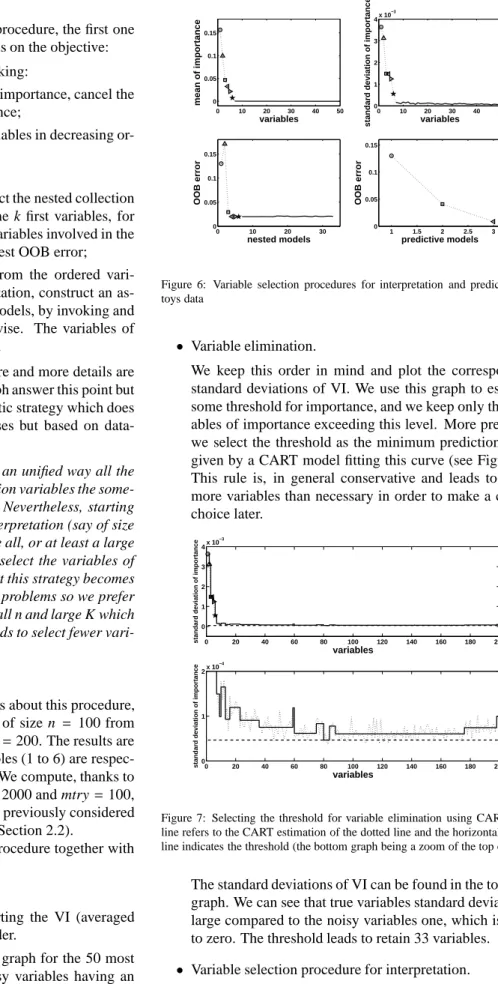
Figure 6: Variable selection procedures for interpretation and prediction for toys data
• Variable elimination.
We keep this order in mind and plot the corresponding standard deviations of VI. We use this graph to estimate some threshold for importance, and we keep only the vari-ables of importance exceeding this level. More precisely, we select the threshold as the minimum prediction value given by a CART model fitting this curve (see Figure 7). This rule is, in general conservative and leads to retain more variables than necessary in order to make a careful choice later. 0 20 40 60 80 100 120 140 160 180 200 0 1 2 3 4x 10 −3 variables
standard deviation of importance
0 20 40 60 80 100 120 140 160 180 200 0 1 2x 10 −4 variables
standard deviation of importance
Figure 7: Selecting the threshold for variable elimination using CART. Bold line refers to the CART estimation of the dotted line and the horizontal dashed line indicates the threshold (the bottom graph being a zoom of the top one)
The standard deviations of VI can be found in the top right graph. We can see that true variables standard deviation is large compared to the noisy variables one, which is close to zero. The threshold leads to retain 33 variables.
• Variable selection procedure for interpretation.
Then, we compute OOB error rates of random forests (us-ing default parameters) of the nested models start(us-ing from
the one with only the most important variable, and ending with the one involving all important variables kept previ-ously. The variables of the model leading to the smallest OOB error are selected.
Note that in the bottom left graph the error decreases quickly and reaches its minimum when the first 4 true vari-ables are included in the model. Then it remains constant. We select the model containing 4 of the 6 true variables. More precisely, we select the variables involved in the first model almost leading to the smallest OOB error. The ac-tual minimum is reached with 24 variables.
The expected behavior is non-decreasing as soon as all the
”true” variables have been selected. It is then difficult to
treat in a unified way nearly constant of or slightly increas-ing. In fact, we propose to use an heuristic rule similar to the 1 SE rule of Breiman et al. (1984) used for selection in the cost-complexity pruning procedure.
• Variable selection procedure for prediction.
We perform a sequential variable introduction with test-ing: a variable is added only if the error gain exceeds a threshold. The idea is that the error decrease must be sig-nificantly greater than the average variation obtained by adding noisy variables.
The bottom right graph shows the result of this step, the final model for prediction purpose involves only variables 3, 6 and 5. The threshold is set to the mean of the absolute
values of the first order differentiated OOB errors between
the model with pinter p =4 variables (the first model after
the one we selected for interpretation, see the bottom left
graph) and the one with all the pelim=33 variables :
1
pelim−pinter p
pelimX−1
j=pinter p
|OOB( j+1)−OOB( j)|.
It should be noted that if one wants to estimate the prediction error, since ranking and selection are made on the same set of observations, of course an error evaluation on a test set or using a cross validation scheme should be preferred. It is taken into account in the next section when our results are compared to others.
To evaluate fairly the different prediction errors, we prefer
here to simulate a test set of the same size than the learning set. The test error rate with all (200) variables is about 6% while the one with the 4 variables selected for interpretation is about
4.5%, a little bit smaller. The model with prediction variables 3,
6 and 5 reaches an error of 1%. Repeating the global procedure 10 times on the same data always gave the same interpretation set of variables and the same prediction set, in the same order.
3.3. Highly correlated variables
Let us now apply the procedure on toys data with replicated variables: a first group of variables highly correlated with vari-able 3 and a second one replicated from varivari-able 6 (the most
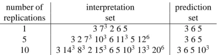
number of interpretation prediction
replications set set
1 3 732 6 5 3 6 5
5 3 2 731036 1135 126 3 6 5
10 3 143832 1536 5 103133206 3 6 5 103
Table 1: Variable selection procedure in presence of highly correlated variables
(augmented toys data) where the expression ijmeans that variable i is a
repli-cation of variable j
important variable of each group). The situations of interest are the same as those considered to produce Figure 4.
Let us comment on Table 1, where the expression ijmeans
that variable i is a replication of variable j.
Interpretation sets do not contain all variables of interest. Particularly we hardly keep replications of variable 6. The rea-son is that even before adding noisy variables to the model the error rate of nested models do increase (or remain constant): when several highly correlated variables are added, the bias re-mains the same while the variance increases. However the pre-diction sets are satisfactory: we always highlight variables 3 and 6 and at most one correlated variable with each of them.
Even if all the variables of interest do not appear in the in-terpretation set, they always appear in the first positions of our ranking according to importance. More precisely the 16 most
important variables in the case of 5 replications are: (3 2 73103
6 1135 126831361661 156146934), and the 26 most
impor-tant variables in the case of 10 replications are: (3 143832 153
6 5 1031332062161131231861 24673266236163256226
1761964 93). Note that the order of the true variables (3 2 6 5
1 4) remains the same in all situations.
4. Experimental results
In this section we experiment the proposed procedure on four high dimensional classification datasets and then finally we ex-amine the results on a standard regression problem to illustrate the versatility of the procedure.
4.1. Prostate data
We apply the variable selection procedure on Prostate data
(for which n=102 and p=6033, see Singh et al. (2002)). The
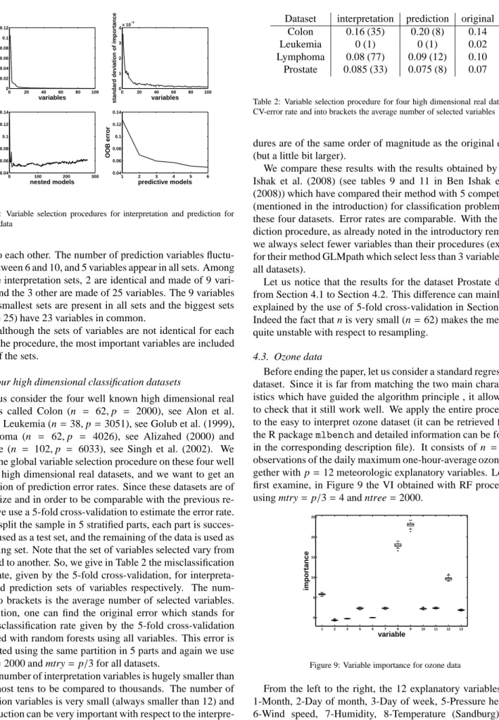
graphs of Figure 8 are obtained as those of Figure 6, except that
for the RF procedure, we use ntree = 2000, mtry = p/3 and
for the bottom left graph, we only plot the 100 most important variables for visibility. The procedure leads to the same picture as previously, except for the OOB rate along the nested models which is less regular. The first point is to notice that the elim-ination step leads to keep only 270 variables. The key point is that the procedure selects 9 variables for interpretation, and 6 variables for prediction. The number of selected variables is
then very much smaller than p=6033.
In addition, to examine the variability of the interpretation and prediction sets the global procedure is repeated five times on the entire Prostate dataset. The five prediction sets are very 7
0 20 40 60 80 100 0 0.02 0.04 0.06 0.08 0.1 0.12 variables mean of importance 0 20 40 60 80 100 0 1 2 3 4x 10 −3 variables
standard deviation of importance
0 100 200 300 0.04 0.06 0.08 0.1 0.12 0.14 nested models OOB error 1 2 3 4 5 6 0.04 0.06 0.08 0.1 0.12 0.14 predictive models OOB error
Figure 8: Variable selection procedures for interpretation and prediction for Prostate data
close to each other. The number of prediction variables fluctu-ates between 6 and 10, and 5 variables appear in all sets. Among the five interpretation sets, 2 are identical and made of 9 vari-ables and the 3 other are made of 25 varivari-ables. The 9 varivari-ables of the smallest sets are present in all sets and the biggest sets (of size 25) have 23 variables in common.
So, although the sets of variables are not identical for each run of the procedure, the most important variables are included in all of the sets.
4.2. Four high dimensional classification datasets
Let us consider the four well known high dimensional real
datasets called Colon (n = 62,p = 2000), see Alon et al.
(1999), Leukemia (n=38,p=3051), see Golub et al. (1999),
Lymphoma (n = 62,p = 4026), see Alizahed (2000) and
Prostate (n = 102,p = 6033), see Singh et al. (2002). We
apply the global variable selection procedure on these four well known high dimensional real datasets, and we want to get an estimation of prediction error rates. Since these datasets are of small size and in order to be comparable with the previous re-sults, we use a 5-fold cross-validation to estimate the error rate. So we split the sample in 5 stratified parts, each part is succes-sively used as a test set, and the remaining of the data is used as a learning set. Note that the set of variables selected vary from one fold to another. So, we give in Table 2 the misclassification error rate, given by the 5-fold cross-validation, for interpreta-tion and predicinterpreta-tion sets of variables respectively. The num-ber into brackets is the average numnum-ber of selected variables. In addition, one can find the original error which stands for the misclassification rate given by the 5-fold cross-validation achieved with random forests using all variables. This error is calculated using the same partition in 5 parts and again we use
ntree=2000 and mtry=p/3 for all datasets.
The number of interpretation variables is hugely smaller than
p, at most tens to be compared to thousands. The number of
prediction variables is very small (always smaller than 12) and the reduction can be very important with respect to the interpre-tation set size. The errors for the two variable selection
proce-Dataset interpretation prediction original
Colon 0.16 (35) 0.20 (8) 0.14
Leukemia 0 (1) 0 (1) 0.02
Lymphoma 0.08 (77) 0.09 (12) 0.10
Prostate 0.085 (33) 0.075 (8) 0.07
Table 2: Variable selection procedure for four high dimensional real datasets. CV-error rate and into brackets the average number of selected variables
dures are of the same order of magnitude as the original error (but a little bit larger).
We compare these results with the results obtained by Ben Ishak et al. (2008) (see tables 9 and 11 in Ben Ishak et al. (2008)) which have compared their method with 5 competitors (mentioned in the introduction) for classification problems on these four datasets. Error rates are comparable. With the pre-diction procedure, as already noted in the introductory remark, we always select fewer variables than their procedures (except for their method GLMpath which select less than 3 variables for all datasets).
Let us notice that the results for the dataset Prostate differ
from Section 4.1 to Section 4.2. This difference can mainly be
explained by the use of 5-fold cross-validation in Section 4.2.
Indeed the fact that n is very small (n=62) makes the method
quite unstable with respect to resampling.
4.3. Ozone data
Before ending the paper, let us consider a standard regression dataset. Since it is far from matching the two main character-istics which have guided the algorithm principle , it allows us to check that it still work well. We apply the entire procedure to the easy to interpret ozone dataset (it can be retrieved from
the R packagemlbenchand detailed information can be found
in the corresponding description file). It consists of n = 366
observations of the daily maximum one-hour-average ozone
to-gether with p=12 meteorologic explanatory variables. Let us
first examine, in Figure 9 the VI obtained with RF procedure
using mtry=p/3=4 and ntree=2000.
1 2 3 5 6 7 8 9 10 11 12 13 0 5 10 15 20 25 importance variable
Figure 9: Variable importance for ozone data
From the left to the right, the 12 explanatory variables are 1-Month, 2-Day of month, 3-Day of week, 5-Pressure height, 6-Wind speed, 7-Humidity, 8-Temperature (Sandburg), 9-Temperature (El Monte), 10-Inversion base height, 11-Pressure
gradient, 12-Inversion base temperature, 13-Visibility. Let us
mention that the variables are numbered exactly as inmlbench,
so the 4th variable is the response one.
Three very sensible groups of variables appear from the most to the least important. First, the two temperatures (8 and 9), the inversion base temperature (12) known to be the best ozone predictors, and the month (1), which is an important predictor since ozone concentration exhibits an heavy seasonal compo-nent. A second group of clearly less important meteorologi-cal variables: pressure height (5), humidity (7), inversion base height (10), pressure gradient (11) and visibility (13). Finally three unimportant variables: day of month (2), day of week (3) of course and more surprisingly wind speed (6). This last fact is classical: wind enter in the model only when ozone pollution arises, otherwise wind and pollution are weakly correlated (see for example Cheze et al. (2003) highlighting this phenomenon using partial estimators).
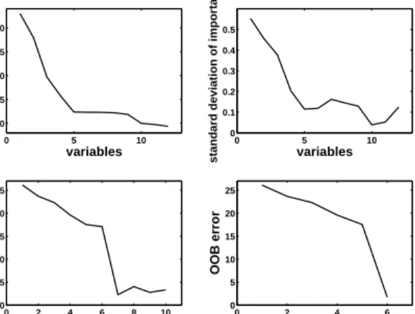
Let us now examine the results of the selection procedures.
0 5 10 0 5 10 15 20 variables mean of importance 0 5 10 0 0.1 0.2 0.3 0.4 0.5 variables
standard deviation of importance
0 2 4 6 8 10 0 5 10 15 20 25 nested models OOB error 0 2 4 6 0 5 10 15 20 25 predictive models OOB error
Figure 10: Variable selection procedures for interpretation and prediction for ozone data
After the first elimination step, the 2 variables of negative importance are canceled, as expected.
Therefore we keep 10 variables for interpretation step and then the model with 7 variables is then selected and it contains all the most important variables: (9 8 12 1 11 7 5).
For the prediction procedure, the model is the same except one more variable is eliminated: humidity (7) .
In addition, when different values for mtry are considered,
the most important 4 variables (9 8 12 1) highlighted by the VI index, are selected and appear in the same order. The variable 5 also always appears but another one can appear after of before.
5. Discussion
Of course, one of the main open issue about random forests is to elucidate from a mathematical point of view its exception-ally attractive performance. In fact, only a small number of
ref-erences deal with this very difficult challenge and, in addition
to bagging theoretical examination by B¨uhlmann et al. (2002),
only purely random forests, a simple version of random forests, is considered. Purely random forests have been introduced by Cutler et al. (2001) for classification problems and then studied by Breiman (2004), but the results are somewhat preliminary. More recently Biau et al. (2008) obtained the first well stated consistency type results.
From a practical perspective, surprisingly, this simplified and essentially not data-driven strategy seems to perform well, at least for prediction purpose (see Cutler et al. (2001)) and, of course, can be handled theoretically in a easier way. Neverthe-less, it should be interesting to check that the same conclusions hold for variable importance and variable selection tasks.
In addition, it could be interesting to examine some variants of random forests which, at the contrary, try to take into ac-count more information. Let us give for example two ideas. The first is about pruning: why pruning is not used for indi-vidual trees? Of course, from the computational point of view the answer is obvious and for prediction performance,
averag-ing eliminate the negative effects of individual overfitting. But
from the two other previously mentioned statistical problems, prediction and variable selection, it remains unclear. The sec-ond remark is about the random feature selection step. The most widely used version of RF selects randomly mtry input variables according to the discrete uniform distribution. Two variants can be suggested: the first is to select random inputs according to a distribution coming from a preliminary ranking given by a pilot estimator; the second one is to adaptively up-date this distribution taking profit of the ranking based on the current forest which is then more and more accurate.
Finally, let us mention an application currently in progress for fMRI brain activity classification (see Genuer et al. (2010)).
This is a typical situation where n << p, with a lot of highly
correlated variables and where the two objectives have to be addressed: find the most activated (whole) regions of the brain, and build a predictive model involving only a few voxels of the brain. An interesting aspect for us will be the feedback given by specialists, needed to interpret the set of variables found by our algorithm. In addition a lot of well known methods have already been used for these data, so fair comparisons will be easy.
References
Alizadeh, A.A., 2000. Distinct types of diffues large b-cell lymphoma identified
by gene expression profiling. Nature. 403, 503-511.
Alon, U., Barkai N., Notterman, D.A., Gish, K., Ybarra, S., Mack D., Levine, A.J., 1999. Broad patterns of gene expression revealed by clustering analysis of tumor and normal colon tissues probed by oligonucleotide arrays. Proc. Natl. Acad. Sci. U.S.A., 96(12), 6745-6750.
Archer, K.J., Kimes, R.V., 2008. Empirical characterization of random forest variable importance measures. Computational Statistics & Data Analysis. 52, 2249-2260.
Ben Ishak, A., Ghattas, B., 2008. S´election de variables pour la classification binaire en grande dimension : comparaisons et application aux donn´ees de biopuces. Journal de la SFdS. 149(3), 43-66.
Biau, G., Devroye, L., Lugosi, G., 2008. Consistency of random forests and other averaging classifiers. Journal of Machine Learning Research. 9, 2039-2057.
Breiman, L., Friedman, J.H., Olshen, R.A., Stone, C.J., 1984. Classification And Regression Trees, Chapman & Hall, New York.
Breiman, L., 1996. Bagging predictors. Machine Learning. 26(2), 123-140. Breiman, L., 2001. Random Forests. Machine Learning. 45, 5-32.
Breiman, L., 2004. Consistency for a simple model of Random Forests. Tech-nical Report 670. Berkeley.
Breiman, L., Cutler, A., 2005. Random Forests. Berkeley.
http://www.stat.berkeley.edu/users/breiman/RandomForests/.
B¨uhlmann, P., Yu, B., 2002. Analyzing Bagging. The Annals of Statistics. 30(4), 927-961.
Cheze, N., Poggi, J.M., Portier, B., 2003. Partial and Recombined Estima-tors for Nonlinear Additive Models. Statistical Inference for Stochastic Pro-cesses. Vol. 6, 2, 155-197.
Cutler, A., Zhao, G., 2001. Pert - Perfect random tree ensembles. Computing Science and Statistics. 33, 490-497.
D´ıaz-Uriarte, R., Alvarez de Andr´es, S., 2006. Gene Selection and classification of microarray data using random forest. BMC Bioinformatics. 7, 3. Dietterich, T., 1999. An experimental comparison of three methods for
con-structing ensembles of decision trees: Bagging, Boosting and randomiza-tion. Machine Learning. 1-22.
Dietterich, T., 2000. Ensemble Methods in Machine Learning. Lecture Notes in Computer Science. 1857, 1-15.
Efron, B., Hastie, T., Johnstone, I., Tibshirani, R., 2004. Least angle regression. Annals of Statistics. 32(2), 407-499.
Fan, J., Li, R., 2001. Variable selection via nonconcave penalized likelihood and its oracle properties. Journal of the American Statistical Association. 96, 1348-1359.
Fan, J., Lv, J., 2008. Sure independence screening for ultra-high dimensional feature space. J. Roy. Statist. Soc. Ser. B. 70, 849-911.
Variable selection using random forests for fMRI classification data. Unpub-lished manuscript.
Genuer, R., Poggi, J.-M., Tuleau, C., 2008. Random Forests: some
methodological insights. Research report INRIA Saclay, RR-6729.
http://hal.inria.fr/inria-00340725/fr/.
Golub, T.R., Slonim, D.K, Tamayo, P., Huard, C., Gaasenbeek, M., Mesirov, J.P., Coller, H., Loh, M.L., Downing, J.R., Caligiuri, M.A., Bloomfield, C.D., Lander, E.S., 1999. Molecular classification of cancer: Class discov-ery and class prediction by gene expression monitoring. Science. 286, 531-537.
Guyon, I., Weston, J., Barnhill, S., Vapnik, V.N., 2002. Gene selection for can-cer classification using support vector machines. Machine Learning. 46(1-3), 389-422.
Guyon, I., Elisseff, A., 2003. An introduction to variable and feature selection.
Journal of Machine Learning Research. 3, 1157-1182.
Gr¨omping, U., 2006. Relative Importance for Linear Regression in R: The Package relaimpo. Journal of Statistical Software. 17, Issue 1.
Gr¨omping, U., 2007. Estimators of Relative Importance in Linear Regression Based on Variance Decomposition. The American Statistician. 61, 139-147. Hastie, T., Tibshirani, R., Friedman, J., 2001. The Elements of Statistical
Learn-ing, Springer, Berlin; Heidelberg; New York.
Ho, T.K., 1998. The random subspace method for constructing decision forests. IEEE Trans. on Pattern Analysis and Machine Intelligence. 20(8), 832-844. Kohavi, R., John, G.H., 1997. Wrappers for Feature Subset Selection. Artificial
Intelligence. 97(1-2), 273-324.
Liaw, A., Wiener, M., 2002. Classification and Regression by randomForest. R News. 2(3), 18-22.
Park, M.Y., Hastie, T., 2007. An L1 regularization-path algorithm for general-ized linear models. J. Roy. Statist. Soc. Ser. B. 69, 659-677.
Poggi, J.M., Tuleau, C., 2006. Classification supervis´ee en grande dimension. Application `a l’agr´ement de conduite automobile. Revue de Statistique Ap-pliqu´ee. LIV(4), 39-58.
Rakotomamonjy, A., 2003. Variable selection using SVM-based criteria. Jour-nal of Machine Learning Research. 3, 1357-1370.
Singh, D., Febbo, P.G., Ross, K., Jackson, D.G., Manola, J., Ladd, C., Tamayo, P., Renshaw, A.A., D’Amico, A.V., Richie, J.P., Lander, E.S., Loda, M.,
Kantoff, P.W., Golub, T.R., Sellers, W.R., 2002. Gene expression correlates
of clinical prostate cancer behavior. Cancer Cell. 1, 203-209.
Strobl, C., Boulesteix, A.-L., Zeileis, A., Hothorn, T., 2007. Bias in random forest variable importance measures: illustrations, sources and a solution. BMC Bioinformatics. 8, 25.
Strobl, C., Boulesteix, A.-L., Kneib, T., Augustin, T., Zeileis, A., 2008. Con-ditional variable importance for Random Forests. BMC Bioinformatics. 9, 307.
Weston, J., Elisseff, A., Schoelkopf, B., Tipping, M., 2003. Use of the zero
norm with linear models and kernel methods. Journal of Machine Learning Research. 3, 1439-1461.