IFPRI Discussion Paper 00954 February 2010
Agricultural Growth and Investment Options for
Poverty Reduction in Nigeria
Xinshen Diao
Manson Nwafor
Vida Alpuerto
Kamiljon Akramov
Sheu Salau
INTERNATIONAL FOOD POLICY RESEARCH INSTITUTE
The International Food Policy Research Institute (IFPRI) was established in 1975. IFPRI is one of 15 agricultural research centers that receive principal funding from governments, private foundations, and international and regional organizations, most of which are members of the Consultative Group on International Agricultural Research (CGIAR).
FINANCIAL CONTRIBUTORS AND PARTNERS
IFPRI’s research, capacity strengthening, and communications work is made possible by its financial contributors and partners. IFPRI receives its principal funding from governments, private foundations, and international and regional organizations, most of which are members of the Consultative Group on International Agricultural Research (CGIAR). IFPRI gratefully acknowledges the generous unrestricted funding from Australia, Canada, China, Finland, France, Germany, India, Ireland, Italy, Japan,
Netherlands, Norway, South Africa, Sweden, Switzerland, United Kingdom, United States, and World Bank.
AUTHORS
Xinshen Diao, International Food Policy Research Institute
Senior Research Fellow, Development Strategy and Governance Division
Manson Nwafor, International Institute of Tropical Agriculture
Consultant
Vida Alpuerto, International Food Policy Research Institute
Senior Research Assistant, Development Strategy and Governance Division
Kamiljon Akramov, International Food Policy Research Institute
Research Fellow, Development Strategy and Governance Division
Sheu Salau, International Food Policy Research Institute
Senior Research Assistant, Development Strategy and Governance Division
Notices
1 Effective January 2007, the Discussion Paper series within each division and the Director General’s Office of IFPRI
were merged into one IFPRI–wide Discussion Paper series. The new series begins with number 00689, reflecting the prior publication of 688 discussion papers within the dispersed series. The earlier series are available on IFPRI’s websit
2 IFPRI Discussion Papers contain preliminary material and research results. They have not been subject to formal
external reviews managed by IFPRI’s Publications Review Committee but have been reviewed by at least one internal and/or external reviewer. They are circulated in order to stimulate discussion and critical comment.
Contents
Abstract
v
Acknowledgements
vi
Abbreviations and Acronyms
vii
1. Introduction
1
2. Modeling Agricultural Growth and Poverty Reduction
2
3. Poverty Reduction under Nigeria's Current Growth Path
5
4. Accelerating Agricultural Growth and Poverty Reduction
13
5. Public Spending in Agriculture to Meet Accelerated Growth and Poverty Targets
31
6. Linking Agricultural Spending to Farmers’ Responses
50
7. Conclusions
58
Appendix A: Mathematical Presentation of the DCGE Model of Nigeria
61
Appendix B: Estimated Elasticity of Agricultural TFP with Respect to Agricultural and
Nonagricultural Spending
68
List of Tables
1. GDP growth rates in the baseline and CAADP scenarios 6 2. Growth decomposition in the model simulations 9 3. Production targets at the subsectoral level 14 4. Current and potential yields for selected crops 15 5. Crop yield, area and production and CAADP targets and growth rates (national level) 16
6. Model growth scenarios 18
7. Subsectoral-level contributions to agricultural CAADP growth 20 8. Regional-level poverty reduction under the CAADP scenario 23 9. Poverty-growth elasticities and growth multipliers 24 10. Summary of factors affecting priority setting in an agricultural strategy 30 11. GDP and government expenditure growth (%), 1981-2007 36 12. Comparison of federal expenditure data from different sources 37 13. Level of agricultural expenditure at the federal and state levels, 2002-07 39 14. Agricultural and total spending requirements under different scenarios 45
15. Descriptive summary of variables 51
16. Determinants of fertilizer use in Nigeria (Dependent variable = fertilizer use) 54
A.1. DCGE model sets and parameters 61
A.2. DCGE model elasticities, coefficients, and exogenous variables 62
A.3. DCGE model endogenous variables 63
A.4. DCGE model equations 64
A.5. Estimated elasticities of agricultural TFP with respect to agricultural and nonagricultural
spending, 1980-2007 68
List of Figures
1. Poverty rates (%) in the baseline scenario 11 2. Regional poverty rates (%) in the baseline scenario 12 3. National poverty rates (%) under alternative agricultural growth scenarios 22 4. Levels of selected agricultural prices in the CAADP scenario 27 5. Oil revenue, non-oil revenue, and total government revenue deflated by CPI, 1980-2007 33 6. Annual changes in world prices for crude oil, Nigerian government oil revenue, total revenue, and
total expenditures, 1980-2007 33
7. Shares of federal and state government in total government revenue, and share of the Federation
Account in state revenue, 1981-2007 35
8. Share of agricultural expenditure in total expenditure, and ratio of agricultural expenditure to
agricultural GDP, 1981-2007 38
9. Share of agricultural expenditure in total expenditure and share of agriculture in GDP, 1981-2007 40 10. Share of agricultural spending in total spending required for accelerated agricultural growth, 2008-17 46 11. Additional agricultural spending required for accelerated agricultural growth (difference from
ABSTRACT
This study uses an economy-wide, dynamic computable general equilibrium (DCGE) model to analyze the ability of growth in various agricultural subsectors to accelerate overall economic growth and reduce poverty in Nigeria over the next years (2009-17). In addition, econometric methods are used to assess growth requirements in agricultural public spending and the relationship between public services and farmers’ use of modern technology. The DCGE model results show that if certain agricultural subsectors can reach the growth targets set by the Nigerian government, the country will see 9.5 percent annual growth in agriculture and 8.0 percent growth of GDP over the next years. The national poverty rate will fall to 30.8 percent by 2017, more than halving the 1996 poverty rate of 65.6 percent and thereby
accomplishing the first Millennium Development Goal (MDG1). This report emphasizes that in designing an agricultural strategy and prioritizing growth, it is important to consider the following four factors at the subsectoral level: (i) the size of a given subsector in the economy; (ii) the growth-multiplier effects occurring through linkages of the subsector with the rest of the economy; (iii) the subsector-led poverty-reduction-growth elasticity; and (iv) the market opportunities and price effects for individual agricultural products.
In analyzing the public investments that would be required to support a 9.5 percent annual growth in agriculture, this study first estimates the growth elasticity of public investments using historical
spending and agricultural total factor productivity (TFP) growth data. The results show that a 1 percent increase in agricultural spending is associated with a 0.24 percent annual increase in agricultural TFP. With such low elasticity, agricultural investments must grow at 23.8 percent annually to support a 9.5 percent increase in agriculture. However, if the spending efficiency can be improved by 70 percent, the required agricultural investment growth becomes 13.6 percent per year. The study also finds that investments outside agriculture benefit growth in the agricultural sector. Thus, assessments of required growth in agricultural spending should include the indirect effects of nonagricultural investments and emphasize the importance of improving the efficiency of agricultural investments. To further show that efficiency in agricultural spending is critically important to agricultural growth, this study utilizes household-level data to empirically show that access to agricultural services has a significantly positive effect on the use of modern agricultural inputs.
ACKNOWLEDGEMENTS
The authors received a great deal of support from various government agencies and research institutions in Nigeria, allowing all of the necessary information and data to be gathered for this study. In particular, the authors thank Valerie Rhoe, James Sackey, Tewodaj Mogues and Samuel Benin for their useful input and suggestions. The authors also thank Bingxin Yu, Alejandro Nin Pratt, Samuel Benin, and Shenggen Fan for their guidance in the econometric estimation, and an internal reviewer for his/her comments on the first draft of the paper. The views expressed in this paper are those of the authors and do not represent the official positions of the International Food Policy Research Institute (IFPRI) or International Institute of Tropical Agriculture (IITA).
ABBREVIATIONS AND ACRONYMS
BOF Budget Office of the FederationCAADP Comprehensive Africa Agriculture Development Program
CBN Central Bank of Nigeria
DCGE Dynamic Computable General Equilibrium FMA Federal Ministry of Agriculture
FMARD Federal Ministry of Agriculture and Rural Development GFS Government Finance Statistics
IMF International Monetary Fund
MDG Millennium Development Goal
NBS National Bureau of Statistics
NEEDS National Economic Empowerment and Development Strategy NEPAD New Partnership for Africa’s Development
NFSP National Food Security Program NPC National Population Commission
OAGF Office of the Accountant General of the Federation SAM Social Accounting Matrix
1. INTRODUCTION
Poverty remains a challenge in Nigeria’s development efforts. Although the national poverty rate was 54 percent , or 69 million people, in 2004, which was reduced from its highest level in the early 1990s, it is still two times higher than the poverty rate in 1980. On the other hand, relatively impressive economic growth rates were recorded during the 2000-07 period. Compared to the periods of 1990-94 and 1995-99, when the economy grew at 2.6 and 3.0 percent per year, respectively, the annual growth rate of GDP rose to 7.3 percent during 2000-07. This suggests that while economic growth is necessary for the country’s development, it does not automatically impact poverty reduction. Notably, the agricultural sector has been a key driver of recent growth in Nigeria. Between 1990 and 2006, the agricultural and oil sectors
accounted for 47 and 39 percent of national growth, respectively. Despite the high dependence of
government revenues and national export earnings on the oil sector, the agricultural sector has comprised the most important source of growth in recent years. Furthermore, as agriculture is the single largest employer among sectors (70 percent of labor force) (NBS 2006) and labor is the main and sometimes only asset for the poor (Agenor et al. 2003), the agricultural sector outperforms all other sectors in reducing poverty.
In recognition of the importance of the agricultural sector in Nigeria, the government has initiated and endorsed many national and international projects, programs and policies aimed at rapidly growing the sector, and thereby reducing poverty. These include the National Economic Empowerment and Development Strategies (NEEDS and NEEDS II), the implementation of the Comprehensive Africa Agriculture Development Program (CAADP) and the National Food Security Program (NFSP), as well as product-specific programs, such as the presidential initiatives on cassava, rice and other crops. Motivating pay offs to these programs have been seen; for example, agriculture’s growth rose from 3.5 percent per annum in 1990-99 to 5.9 percent per annum in 2000-07, and poverty decreased from 65.6 percent in 1996 to 54.4 percent in 2004. Despite these accomplishments, however, further efforts will be necessary if we hope to lift more people out of poverty and meet the first Millennium Development Goal (MDG1) of halving the proportion of people who live under the poverty line, with incomes of less than US$1 dollar per day.
Against this background, the present study analyzes the agricultural growth and investment options that could support the formation of a more comprehensive rural development component under NEEDS II, in alignment with the principles and objectives collectively defined by African countries as part of the broader NEPAD agenda. In particular, the study seeks to position Nigeria’s agricultural sector and rural economy within NEEDS II. For these purposes and to assist policy makers and other
stakeholders in making informed long-term decisions, we herein develop an economy-wide, dynamic computable general equilibrium (DCGE) model for Nigeria, and use it to analyze the linkages and trade-offs between economic growth and poverty reduction at both the macro- and microeconomic levels. After introducing the DCGE model in the next section, we have considered two scenarios using the DCGE model. In the first scenario in Section 3, we consider a growth path following the country's current growth trends and we define it as a baseline scenario. In the second scenario in Section 4 we simulate a growth path along which growth at the agricultural subsector levels is accelerated to meet with the targets set by the government. Additional growth is assumed from increases in productivity instead of more land expansion. In this scenario we also evaluate whether subsector level targets can allow the country's total agriculture to grow at 10 percent annually, a growth target defined in NEEDS II. We call this scenario a 'CAADP scenario' though the targeted 10 percent of agricultural growth is much higher than the 6 percent of CAADP goal. In Section 5, we attempt to quantify the public resources that should be funneled to the agricultural sector in order to achieve the government’s stated development goals, while in Section 6 we turn to analyze the linkages between public services and farmers’ use of modern technology. Section 7 concludes the paper with major findings and policy implications.
2. MODELING AGRICULTURAL GROWTH AND POVERTY REDUCTION
1 Previous CGE Models for NigeriaPreviously, CGE modeling has been used to study the Nigerian economy and analyze the ability of agriculture and its different subsectors to achieve various poverty and growth goals. These papers include those by Iwayemi (1995), the UNDP (1995b), Ajakaiye and Olomola (2003) of the Nigerian Institute of Social and Economic Research (NISER), and the analysis done for NEEDS II using the National Planning Commission-Center for Econometric and Allied Research (NPC-CEAR) model (NPC 2007). All of these models were done at the national level (i.e., they were not disaggregated to the levels of the various regional economies) and were relatively aggregated in their sectoral structures. Iwayemi (1995), for example, designed a quasi-CGE model to check the consistency of targets laid out in the first perspective plan developed during the 1990s (it is not clear whether this model was actually used to analyze policy issues). The UNDP (1995b) model was a follow up to that of Iwayemi (1995), and used a Social Accounting Matrix (SAM) that comprised 52 sectors, including some agricultural subsectors. However, we were unable to find any policy analysis performed using this model.
In contrast, the NISER (Ajakaiye and Olomola 2003) and NPC-CEAR (NPC 2007) models have been successfully used to analyze various economic targets in relation to overall growth targets. The NISER model projected the expected growth rates of the economy between 2001 and 2015 based on assumptions of future levels of key economic variables, namely the exchange rate, interest rate, minimum wage, government capital expenditure, exports, and investments. The analysis for NEEDS II using the NPC-CEAR model focused on estimating the sectoral growth rates required to achieve 10 percent growth in the economy for 2008-11.
While the latter two studies linked national growth to that in economic variables and different sectors, they did not consider the agricultural sector in detail and did not fully assess the relative roles that the different agriculture subsectors can play in accelerating agricultural and economy-wide growth. With regard to poverty impacts, the NISER model was limited to concluding that the daily per capita income would increase from US$1 in 2001 to US$4.4 in 2015 if the assumed levels of the economic variables were met; however, it is not clear how this result was obtained from the model. As for NEEDS II, the existing modeling analysis did not clearly distinguish what poverty impact would be expected from the ‘required’ 10 percent economic growth. Another limitation for both reports was that the analysis could not be applied to disaggregated households, and the papers therefore failed to discuss the impact of growth on different types of rural and urban households.
The Dynamic General Equilibrium (DCGE) Model and a Microsimulation Module for Nigeria
A standard static CGE model was developed in the early 2000s at the International Food Policy Research Institute (IFPRI), as documented by Lofgren (2001). The recursive dynamic version of the CGE model incorporates a series of dynamic factors into the standard static CGE model. An early version of the DCGE model was first developed by Thurlow (2004), and its recent application to two country case studies (in Zambia and Uganda) was done by Diao et al. (2007). We herein develop a DCGE model for Nigeria in this study. The DCGE model captures the trade-offs and synergies that come from accelerating growth in various agricultural subsectors, as well as the economic inter-linkages between agriculture and the rest of the economy. Although our study focuses on the agricultural sector, the DCGE model for Nigeria also contains information on nonagricultural sectors. The model examines 62 subsectors in total, more than half of which are in agriculture. The examined agricultural crops fall into four broad groups: (i) cereal crops, including rice, wheat, maize, sorghum, and millet; (ii) root crops, such as cassava, yam,
soybeans, other oil crops, vegetables for domestic use, and fruits for domestic use; and (iv) higher-value export-oriented crops, such as cocoa, coffee, cotton, oil palm, vegetables for export, fruits for export, sugar, tobacco, cashew nuts, other nuts, rubber, and other export crops. The DCGE model also identifies four primary livestock sectors, namely: cattle, goats and sheep, poultry, and other livestock. To complete the agricultural sector, the model also includes forestry and fisheries. Most of the agricultural
commodities listed above are not only used for domestic consumption or export, they are also used as intermediate inputs into various processing activities in the manufacturing sector. The ten agricultural processing activities (including eight food-processing activities) identified in the model comprise the processing of: beef; goat and sheep meat; poultry meat; eggs; milk; other meats; beverages; other foods; textiles; and wood. The agricultural sectors themselves also use inputs produced from nonagricultural sectors, such as fertilizer and transport and trade services for crops.
The DCGE model for Nigeria also captures regional heterogeneity. Rural agricultural production is disaggregated across six zones in Nigeria, with representative farmers engaging in different crop- and livestock-production strategies across zones. Therefore, the model is calibrated to the initial agricultural structure at the zonal level. The representative farmers within each zone respond to changes in production technology, commodity demand, and commodity prices by making decisions on how to allocate land and family labor across the different crops and livestock subsectors, and whether or not to purchase other inputs (e.g., hired labor, capital, and intermediate inputs) in order to maximize their net incomes from agriculture. The allocation of labor is also determined by the opportunity to participate in nonagricultural activities, which primarily occur in urban areas or rural towns. Such opportunities are modeled from the demand side, in that the representative producers in the nonagricultural sectors, when making their production decisions, decide on the amount of labor to be hired in, taking market wage rates as given. Thus, by capturing production structure at the subnational level, the DCGE model effectively integrates the information on different agents and activities into an economy-wide model that can be used to assess growth effects at the national level. The DCGE model for Nigeria is therefore an ideal tool for capturing the growth linkages, income effects, and price effects resulting from growth acceleration in different agricultural sectors. Additional detail on the DCGE model is available in Appendix A.
Finally, the DCGE model endogenously estimates the impact of alternative growth paths on the incomes of various household groups. These household groups are defined based on the six zones and rural or urban location, for a total of 12 representative household groups. Each household group is aggregated from the Nigeria Living Standards Survey (NLSS) 2003/04 such that all households sampled in NLSS 2003/04 can be linked directly to their corresponding representative household in the DCGE model. The microsimulation module2
The Data
, which contains all households sampled in NLSS 2003/04, is linked to the DCGE model. In this macro-to-micro linkage, changes in representative households’ consumption patterns and prices in the DCGE model are passed down to their corresponding households in the microsimulation module (containing all sampled households from NLSS 2003/04, where the total consumption expenditure for each sample household is recalculated from the new level of consumption on a by-commodity basis. The new level of per capita expenditure obtained for each survey household is then compared to the official poverty line, and standard poverty measures are re-calculated. Thus, the poverty measures are consistent with official poverty estimates, while the changes in poverty draw on the analyzed across-group consumption patterns, income distributions, and poverty rates.
The data used to calibrate the base year of the DCGE model used in this study are drawn from a variety of sources. The core dataset underlying the DCGE model is a SAM constructed in 2006 using data from the national accounts, trade data from the Nigeria Bureau of Statistics (NBS), and balance-of-payment information from the Central Bank of Nigeria (CBN). National- and state-level data on agricultural production, agricultural yield, and market prices come from the Federal Ministry of Agriculture and Rural
Development (FMARD). In cases where production data are unavailable for certain crops (e.g., horticulture), information is taken from the Food and Agriculture Organization (FAO) of the United Nations. These agricultural production data are disaggregated across the zones by mapping each of the states to the six zones. The DCGE model is therefore consistent with official agricultural production levels and yields at the zonal level. Nonagricultural production, employment, and other value-added component of national-level sectoral GDP data are compiled from national account tables (NBS 2007a). On the demand side, the information on industrial technologies (e.g., intermediate and factor demand) comes from an earlier SAM for Nigeria (UNDP 1995b), while the income and expenditure patterns for the various household groups are taken from NLSS 2003/04. The DCGE model is therefore based on the most recent available data for Nigeria and represents the country’s economy in 2006.
3. POVERTY REDUCTION UNDER NIGERIA'S CURRENT GROWTH PATH
Design of a Baseline Simulation to Capture Growth TrendsThe dynamic CGE model developed for this study is first used to simulate a base-run that captures Nigeria’s current growth and poverty reduction trends, taking into account the recent changes in the country’s external environment (e.g., the global financial crisis and the sharp decline in world crude oil prices). These external changes are expected to negatively affect the Nigerian economy’s performance in the near future, as crude oil accounts for 37 percent of national total GDP. History shows that the
Nigerian economy is very vulnerable to oil price shocks, which impact the effective exchange rate, government expenditures, money supplies, trade, and inflation (Akpan 2009). Given that both the global financial crisis and the declines in world crude oil prices are expected to last for some time, the base-run simulation considers a modest, targeted economic growth rate that is lower than the 7.6 percent annual growth recorded during the period of 2002-07 (CBN 2009). Measured in real terms, although the crude oil sector’s GDP grew at only 4.4 percent annually during this period, due to rising world oil prices, the sector’s contribution to overall economic growth was mainly channeled through increased oil revenues. Given that this factor is unlikely to play a key positive role in stimulating growth in the present and near future, and some of its effects may even become negative (e.g., declines in oil revenue may force the government to increase the allocation of growth-stimulating funds), the base-run simulation targets a modest annual GDP growth rate of 6.5 percent over the next years (2008-17) (Table 1). While this growth rate is lower than the recent performance of the Nigerian economy, it is still relatively high considering the current external conditions worldwide. Moreover, this growth rate is higher than the historical average growth rate if a longer period is considered. For example, the average annual GDP growth rate during the period 1995-2007 was 5.5 percent (CBN 2009).
The base-run also considers relatively modest growth in the agricultural sector. In addition to the reasons noted above to explain our growth projection of the general economy, another factor reminds us to be cautious when projecting agricultural growth: Although the national account tables show high-level growth (6.7 percent) in agricultural GDP between 2002 and 2007, such a rapid growth in agricultural GDP is not consistent with individual crop production data obtained from FMA or the market situation (e.g., the price situation) for the major food crops in the domestic markets. In terms of the production reported by FMA for certain smallholder-produced crops, the average annual growth rate was 5.5 percent in 2000-06. Such growth was primarily driven by area expansion, whereas yield increase-driven growth was very modest. For example, the FMA data show that the annual yield-growth rates for cassava, sorghum, millet, and maize, were 0.9, 0.3, 0.4, and 0.8 percent, respectively, for this period. These four major food crops together account for more than 50 percent of agricultural area in Nigeria at present. Given this historical perspective, we use a set of more realistic growth rates for each individual crop and livestock product, and apply an annual agricultural growth rate of 5.7 percent (similar to that of 2000-07) in the baseline scenario.3
3 The NBS is aware of potential problems in agricultural crop GDP calculations during this period, particularly in 2002, as
shown below:
Year Crop production GDP (1990 constant prices in billions of Naira) Annual growth rate (%)
1997 87.4 1998 90.8 3.9 1999 95.5 5.2 2000 98.4 3.0 2001 102.1 3.8 2002 168.8 65.3 2003 181.2 7.3 2004 192.4 6.2 2005 206.2 7.2 2006 221.6 7.5 Source: NBS (2007).
Table 1. GDP growth rates in the baseline and CAADP scenarios
Share of GDP Annual growth rate, 2008-17 (%)
In 2006 Baseline CAADP scenario
Total GDP 19,909 6.5 8.0 (billion Naira) Agriculture 29.7 5.7 9.5 Cereals 7.7 5.4 9.5 Rice 2.6 5.1 10.2 Wheat 0.0 5.0 25.9 Maize 2.2 7.3 12.0 Sorghum 1.6 4.0 5.7 Millet 1.3 4.2 5.7 Root crops 9.4 6.0 8.9 Cassava 4.4 5.6 8.7 Yams 3.9 6.4 9.3 Cocoyams 0.2 4.7 6.0 Potatoes 0.3 8.8 12.4 Sweet potatoes 0.6 4.7 7.0
Other food crops 7.6 5.7 8.1
Plantains 0.6 3.8 4.9 Beans 1.0 5.3 7.6 Groundnuts 1.1 5.5 7.7 Soybeans 1.1 5.7 8.5 Other oilseeds 0.1 4.5 6.3 Vegetables 1.8 6.1 8.6 Fruits 1.6 6.4 8.7 High-value crops 1.5 5.6 17.6 Cocoa 0.1 3.9 4.9 Coffee 0.2 6.1 8.8 Cotton 0.1 5.2 11.2 Oil palm 0.5 3.8 5.7 Sugar 0.3 7.3 33.1 Tobacco 0.1 6.8 10.0 Nuts 0.0 5.7 7.9 Cashew nuts 0.004 5.7 7.7 Rubber 0.2 6.1 6.1
Other export crops 0.017 8.5 12.8
Livestock 1.9 5.4 6.9
Cattle 0.6 5.5 6.4
Goats & sheep 0.9 5.1 6.5
Table 1. Continued
Share of GDP Annual growth rate, 2008-17 (%)
In 2006 Baseline CAADP scenario
Other agriculture 1.6 5.8 10.9 Forestry 0.5 4.2 5.7 Fisheries 1.0 6.5 12.9 Mining 34.6 3.7 3.7 Cruel oil 34.5 3.7 3.7 Other mining 0.1 3.7 3.7 Manufacturing 6.9 6.7 7.4 Beef 0.6 6.2 7.6
Goat & sheep meat 2.2 6.0 7.2
Poultry meat 0.2 8.2 13.3 Eggs 0.03 7.3 10.7 Milk 0.01 7.5 9.9 Other meats 0.02 5.7 5.9 Beverages 0.3 7.3 7.7 Other foods 0.4 8.1 8.6 Textiles 0.5 7.8 8.3 Wood processing 0.3 7.9 8.8 Electronic manufacturing 0.9 6.4 5.4 Other manufacturing 1.1 6.5 6.0 Oil refining 0.3 6.2 6.2 Other industries 4.3 8.5 8.8 Construction 1.2 9.2 9.5 Utility 3.1 8.2 8.6 Services 24.5 9.6 10.7 Road transportation 2.2 14.9 16.3 Other transportation 0.1 15.1 16.1 Trade 8.3 9.8 11.4
Hotels and restaurants 1.2 8.2 9.1
Communication 0.8 13.2 14.1
Finance and other business services 1.8 13.8 14.4
Real estate 2.6 7.5 7.5
Education 1.3 5.8 6.5
Health 0.6 6.0 6.8
Public services 4.6 4.8 5.6
Other private services 1.0 7.2 7.4
Factors Determining Growth in the Model
To model a realistic baseline, it is also important to be aware of the growth sources across sectors and for different input factors. In the model, economic growth results from increases in labor supply, land expansion, capital accumulation, and productivity changes. We assume that the growth in total labor supply is consistent with the projected annual population growth of 3.0 percent.4
The total zonal-level land expansion for 2009-17 is exogenously determined based on the recent trends observed by FMARD (2007). The assumed initial expansion rate of 5.2 percent per year is consistent with FMARD data recorded in 2001-06. After 2011, land expansion is assumed to fall to 4.2 percent, which is still relatively high. The average annual growth rate of land expansion across the modeled period is 4.4 percent (Table 2). Due to a lack of information regarding land expansion potential at the zonal level, we have to assume a uniform growth rate across the six zones. Given that agricultural production activities are modeled at the zonal level, it will be straightforward to adopt different land expansion rates once such information is available.
Three types of labor are distinguished in the model: (i) rural family labor employed in agricultural production only; (ii) unskilled labor that can move freely across sectors (i.e., between agricultural and nonagricultural production); and (iii) skilled labor employed only in the nonagricultural sector. Taking into account a more rapid growth in labor supply to the nonagricultural sector, we assume that the annual growth rate for rural family labor is 2.0 percent, while the growth rates in unskilled and skilled labor (the two economy-wide labor categories) are 3.3 and 3.4 percent, respectively.
Capital accumulation is an endogenous outcome of savings and investments, which are modeled recursively in our model. Investments are financed through private and government savings. Private savings are determined by a fixed proportion of total income (an endogenous variable) received by each of the 12 representative households, while government savings is the difference between government income (an endogenous variable) and total non-investment spending (an exogenous variable). Both private and public savings rates are calibrated to the 2006 SAM. Investments are also affected by foreign capital flows. Since Nigeria has experienced a trade surplus in recent years, the net foreign capital inflows are negative in the model (indicating capital outflow). In the recursive dynamic model, this outflow is an exogenous variable whose growth is assumed to decline due to the expected slow growth in oil exports. This assumption brings the expectation that more oil revenues will be used to finance domestic
investments, instead of purchasing foreign bonds or investing in foreign capital markets (as seen in the current situation). In the baseline, capital accumulates at 4.6 percent annually in real terms after a 5.0 percent depreciation (Table 2).
While the total factor supply grows either exogenously (labor and land) or endogenously (capital), its sectoral-level demand is endogenous. Factor demand is determined by competition in the factor markets, and by the profitability of each individual sector. The third part of Table 2 shows the growth rate in aggregate labor and capital demand for agriculture and nonagriculture. As can be seen in the table, the demand for total agricultural labor grows at 2.2 percent annually, while that for the
nonagricultural sector grows at 3.7 percent annually. The growth rate of total agricultural capital demand is higher than that for total nonagricultural capital demand (6.7 percent vs. 4.5 percent, respectively); however, since agricultural capital accounts for a very small portion of total capital input, even given rapid growth the share of capital in agricultural GDP remains very small (< 5.0 percent of agricultural GDP; by comparison, capital accounts for more than 60 percent of nonagricultural GDP, as shown in the first part of Table 2).
Table 2. Growth decomposition in the model simulations
GDP AgGDP NagGDP
Baseline CAADP Baseline CAADP Baseline CAADP Annual output growth rate (%) 6.5 8.0 5.7 9.5 6.8 7.4 Share in the economy (%) In GDP In AgGDP In NagGDP
Land 11.0 37.0
Labor 45.7 59.4 39.9
Capital 43.3 3.6 60.1
Contribution to growth (%) To GDP growth To AgGDP growth To NagGDP growth Baseline CAADP Baseline CAADP Baseline CAADP
Land 9.5 9.8 33.3 24.7
Labor 20.2 16.2 21.2 12.4 21.7 20.1 Capital 31.6 25.9 5.0 3.3 41.2 38.6 Total Factor Productivity (TFP) 38.7 48.1 40.6 59.6 37.1 41.2 Annual input and TFP growth rate (%) Baseline CAADP
Land 4.8 5.7
Labor 3.0 3.0
Agricultural (ag) labor 2.2 2.1 Nonagricultural (nag) labor 3.7 3.7
Capital 4.6 4.7 Ag capital 6.7 7.1 Nag capital 4.5 4.6 TFP 2.5 3.8 Ag TFP 2.3 5.6 Nag TFP 2.5 3.0
Source: Nigerian DCGE model results.
It is impossible to have sustainable growth without a change in productivity. The model assumes that total factor productivity (TFP) grows exogenously at the sectoral level across all six zones. The TFP growth rate is drawn from historical data and is based on the yield-growth rate for crop sectors, and on sectoral value-added growth in the case of non-crop sectors.
While productivity growth is a driving force of growth at the sectoral level, growth is also affected by demand. If the supply of a specific commodity cannot find enough demand in either the domestic or foreign markets, the price for this commodity in the domestic market falls, subsequently reducing the factor demanded by the production of this commodity and lowering its growth rate.
We calculate the contribution of the factors and productivities to overall economic growth, as shown in Table 2. The contribution of a given factor to growth depends on its growth rate and share in adding value. For the economy as whole, land accounts for 11.0 percent of GDP, while labor and capital account for 45.7 and 43.3 percent, respectively. In terms of GDP growth in the baseline scenario, 61.3 percent of growth is due to factor accumulation, while 38.7 percent comes from TFP growth (Table 2, second part). We also examine the contributions to growth in agricultural and nonagricultural GDP. In the baseline scenario, almost 60 percent of agricultural growth is due to land expansion, increased labor supply, and capital accumulation, whereas productivity increases explain the remaining 40 percent of growth. Within the crop sectors, productivity gains come both from yield improvements and more efficient allocations of land to the production of higher-return commodities.
Growth at the Subsectoral Level
While the base-run models overall annual growth in GDP and the agricultural sector at 6.5 and 5.7 percent, respectively, during 2008-17, the growth rates differ across sectors. Specifically, input allocation across sectors differs over time due to differences in sectoral productivity growth and price changes. For example, although agricultural GDP grows at 5.7 percent annually, the growth in total cereal value-added is 5.4 percent, while those in rice, maize, and Irish potato production are 5.1, 7.3, and 8.8 percent,
respectively (Table 1).
Table 1 presents the base-run GDP growth rates for the subsectors included in the model, as well as for some subsector groups. All of these growth rates are the endogenous results of the model. The first column of the table gives the size of each sector as a share of the total GDP, representing the initial structure of the Nigerian economy in 2006.
Poverty Reduction Outcome in the Baseline Simulation
The poverty-reduction impact of the modeled economic growth is analyzed using a microsimulation module that includes all households sampled in NLSS 2003/04. By taking into account micro-level consumption patterns across households, we determine demand changes at the
individual-food-commodity level for each sampled household, by linking such demand with the representative household demand for the same commodity in the DCGE model. As discussed in Section 2, the representative households are aggregated from the sample households (based on the six zones and by rural/urban location). Although such top-down linkages between the DCGE model and the microsimulation module do not allow us to capture the distributional effects of growth within each zone’s rural or urban household group, we do capture certain differential welfare effects across zones and between rural and urban
households.
Before we start the exercise, we assess the impact of growth on poverty reduction using historical national-level poverty data available for 1980, 1985, 1992, 1996, and 2004. Because the poverty rate of 65.6 percent in 1996 was much higher than that in 1992 (42.7 percent), it is difficult to perform a trend analysis over a longer period. For this reason, we focus on the poverty rates in the recent period between 1996 (in which the poverty rate was 65.6 percent) and 2004 (54.4 percent), and compare them with actual per capita GDP growth over the same period. While the annual growth rate of GDP per capita was 2.5 percent (calculated from the CBN’s annual GDP growth rate of 5.5 percent and the annual population growth rate of 3.0 percent during this period), the total decline in the poverty rate was only 11.2
percentage points over these seven years (or 2.3 percent per year). By comparing the total decline in the national poverty rate (i.e. 2004’s poverty rate is 17 percent, not percentage points, lower than that in 1996) with the total growth in per capita GDP (22 percent) across the same seven years, we derive a poverty-reduction-growth elasticity of –0.78.5
5 The poverty–growth elasticity used in this study measures the responsiveness of the poverty rate to changes in the per
capita GDP growth rate. The formula for this elasticity is:
This indicates that for a 1 percent growth in per capita GDP in Nigeria between 1996 and 2004, the poverty rate fell by 0.78 percent from the 1996 level. Although the elasticity is affected by the initial poverty rate (which was high in 1996) and the pattern of income distribution around the poverty income line, such elasticity is comparable with that obtained for other African countries (See Diao et al. 2007).
,
where and are the average annual changes (from the base year) in the poverty headcount rate and the level of per
pc 0 0 0 pc pc pc 0 GDP P P P GDP GDP GDP P ∆ ∆ = ⋅ ∆ ∆ P ∆ ∆GDP
We also use the same formula to calculate the poverty-growth elasticity from the results of the baseline simulation, and obtain a similar elasticity of -0.851. That is to say, for a 1 percent of growth in per capita GDP over the next ten years along the base-run path, the national poverty rate will fall by 0.851 percent. Given such elasticity, our poverty analysis shows that annual growths of 6.5 percent in total GDP and 5.7 percent in agricultural GDP over the next years (2008-17), together with a 3.0 percent annual population growth in the same period, will decrease the national poverty rate from 51.6 percent in 20086
Figure 1. Poverty rates (%) in the baseline scenario
to 39.4 percent by 2017 (Figure 1). However, although this poverty rate is already lower than that seen in 1992 (42.7 percent), given the 3.0 percent population growth per year, the number of poor people will actually increase over time. The base-run result shows that there will be 287,000 more poor people in Nigeria in 2017 versus 2008.
Source: Nigerian DCGE model results.
The base-run also generates national-level rural and urban poverty rates (Figure 1), as well as zonal-level rates for the six regions (Figure 2). The NLSS 2003/04 data show that in 2004, poverty was worse in rural areas (63.3 percent) than in urban areas (43.2 percent). These poverty rates are the starting points in the model and are used to simulate the poverty rates in 2008 and beyond. As shown in Figure 1, given a 6.5 percent annual growth in total GDP and 5.7 percent growth in agricultural GDP, the poverty rates fall to 47.9 and 29.4 percent in rural and urban areas, respectively, by 2017. Because the absolute percentage-point decline for the rural group is slightly higher than that for the urban group (12 vs. 11 percentage points, respectively, between 2008 and 2017), the poverty gap between the rural and urban regions becomes smaller (20.1 percentage points in 2008 vs. 18.5 percentage points in 2017).
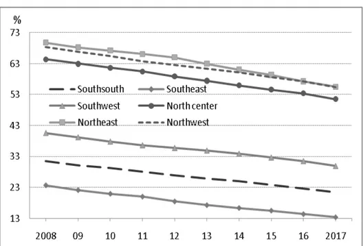
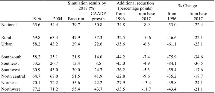
As discussed in Section 1, the spatial pattern of poverty distribution in Nigeria shows a south-to-north disparity; in 2004, the three southern regions had poverty rates between 26.7 to 43.0 percent, while the northern regions had poverty rates between 67.0 to 72.2 percent. This type of regional gap in poverty will continue through the next years. The base-run model results show that the poverty rates in the three southern regions will fall between 13.4-30.0 percent by 2017, but will remain high between 51.5 to 55.6 percent in the three northern regions (Figure 2).
Figure 2. Regional poverty rates (%) in the baseline scenario
4. ACCELERATING AGRICULTURAL GROWTH AND POVERTY REDUCTION
Going Beyond the CAADP Agricultural Growth TargetIn the previous section, we describe the results of the base-run scenario and estimate the
poverty-reduction impact of a growth path that takes into account both Nigeria’s past growth experiences and our present external conditions. In this section, we examine the potential contribution of different agricultural subsectors toward helping Nigeria achieve a much higher overall rate of agricultural growth.
The CAADP initiative has set a 6 percent annual agricultural growth rate as a target for African countries. Considering that recent agricultural growth in Nigeria has been close to this CAADP target, the government has set a higher growth target of 10 percent. To meet the 10 percent target for overall
agricultural growth, a set of sector-specific growth targets have been defined for the production of major crops and livestock (FMARD 2008). Most of these subsectoral-level targets specify the sector’s output; growth in productivity (or yield) is only mentioned for cassava. Table 3 summarizes the current levels and production targets at the subsectoral level, both obtained from a draft of FMARD (2008).
Given that there is a large yield gap between the current and maximum levels for most crops (Table 4), the potential for agricultural growth in Nigeria is high. However, considering that FMARD (2008) addresses only a relatively short period, the targeted growth seems to be unrealistic for most food crops. According to a report published by ReSAKSS WA (2009), potential yield predictions are often based on growth under the idealized conditions of controlled field trials. Thus, it is unlikely that farmers will be able to achieve such yields at the national level over the short period under consideration. It will also be difficult to realize nationwide adoption of the improved seeds and modern technologies that are needed to reach such high yield potentials. It does not seem that these constraints have been taken into account when the production targets were designed. For example, in FMARD (2008), cassava yield and production are both targeted to double nationwide over a period of four years (2008-11), for annual growth rates of 19.5 percent. When we design a scenario that we call the “CAADP growth scenario,” which is based on the targets set in FMARD (2008), we apply such targets to a period from 2009 to 2017, giving farmers a longer timeframe to meet similar targets. For example, in the case of cassava, the annual growth rate becomes about 8.9 percent in our model. The second part of Table 3 gives the modeled growth rates for crop and livestock production, which we set using the government’s targets.
FMARD (2008) includes production targets for ten crops, five livestock products, and the fishery sector. To model the accelerated growth in these crops and livestock production subsectors under the CAADP scenario, we assume additional land expansion for some crops (rice, wheat, cocoa, sugar and oil palm), while for the other crops, as well as livestock and fisheries, additional growth is assumed to come only from productivity improvement (e.g., yield increases in the case of crops). While production targets are not available for many of the crops included in the model, a number of these are large subsectors in the agricultural economy (e.g., maize, sorghum, yams, pulses and oilseeds); therefore, the simulation also assumes additional productivity growth for these crops.
Table 3. Production targets at the subsectoral level
Target defined in NFSP DCGE model results
Current
level Level by 2011 Total increase Annual growth Level by Total increase Annual growth
Million mt Million mt % (08-11, %) 2017 (06-17, %) (09-17, %) Crops Cassava 49.0 100.0 104.1 19.5 96.0 115.0 8.9 Rice 2.8 5.6 100.0 18.9 22.8 142.0 10.3 Millet 4.0 6.5 62.5 12.9 14.1 64.1 5.7 Wheat 0.1 0.5 614.3 63.5 0.5 548.7 23.1 Sugar 0.2 2.2 1034.0 83.5 33.9 1072.5 31.5 Tomatoes 1.1 2.2 100.0 18.9 11.7 99.6 8.0 Cotton 0.4 1.0 185.7 30.0 2.1 172.7 11.8 Cocoa 0.4 0.7 84.2 16.5 0.7 141.4 10.3 Palm oil 0.8 1.3 50.0 10.7 12.6 74.5 6.4 Palm kernels 0.4 0.6 50.0 10.7 Rubber 0.2 0.3 50.0 10.7 0.6 82.9 6.9
Livestock & fisheries
Poultry 166.0 249.0 50.0 10.7 182.2 110.1 8.6 Goats 52.0 67.6 30.0 6.8 391.6 81.9 6.9 Sheep 33.0 42.9 30.0 6.8 Cattle 16.0 20.0 25.0 5.7 257.8 78.5 6.6 Pigs 6.6 8.3 25.0 5.7 28.7 113.3 8.8 Fisheries 0.5 1.5 200.0 31.6 750.8 189.4 12.5 Agricultural GDP 10.0 -15.0 9.5
Table 4. Current and potential yields for selected crops
Current yield (mt/ha) Potential yield (mt/ha)
Rice 1.9 7.0 Cassava 12.3 28.4 Maize 1.6 4.0 Sorghum 1.1 3.2 Millet 1.1 2.4 Yams 12.3 18.0 Irish Potatoes 7.6 10.5 Soybeans 1.2 2.0 Beniseeds 0.6 1.0 Melons 0.4 0.5 Cocoa 0.2 2.0 Cowpeas 0.5 2.3 Okra 3.1 5.5
Sources: The current yields come from FMARD (2007) and NBS (2005a); the potential yields come from ReSAKSS WA (2009).
Taking maize as an example, data from FMARD (2007) indicates that the current national yield level is around 1.4 metric tons per hectare (mt/ha). Under the base-run scenario, we assume that the average maize yield for the next years will grow at 0.3 percent annually, which is consistent with the yield growth seen in the country during the prior seven years (1999-2006). Given such growth, the maize yield level will unlikely to change over the next years, and growth in maize production will be primarily driven by area expansion. Under the CAADP scenario, we model a slightly more ambitious maize yield
improvement, with an annual growth rate of 2.9 percent per year (Table 5). This implies that the national average maize yield will reach 1.8 mt/ha by 2017. This is still below the potential yield of 4.0 mt/ha that has been achieved in certain experimental projects and farm trials using improved technologies and practices (Valencia and Breth 1999). As discussed above, however, the majority of maximum yields are achieved under ‘ideal’ conditions in agricultural research stations or on-farm trials. These potential yields can only be achieved through access to modern inputs, including the use of improved high-yield seed varieties and new technologies, as well as improved farming practices that differ from the traditional methods that most farmers presently use (ReSAKSS WA 2009). Because maximum yields require better technology, farming knowledge, and market conditions, we deem it unrealistic to assume that such high yields will be realized at the national level in the next years. However, even though we project
conservative crop yields in the CAADP scenario, the annual growth rates required to achieve the target yields are already higher than the historical trends (Table 5). Clearly, it will be a daunting task to achieve the government’s target yields.
Table 5. Crop yield, area and production and CAADP targets and growth rates (national level)
Crop yield Harvested area Production quantity
Initial level Baseline Target CAADP Initial level Share Baseline CAADP Initial level Baseline CAADP mt/ha growth % mt/ha growth % 1000 ha % % % 1000 mt % %
Cereals Rice 1.5 1.1 2.4 5.1 6,214 8.6 4.5 5.0 9,436 5.6 10.3 Wheat 1.1 0.1 1.3 1.8 70 0.1 5.5 20.9 80 5.6 23.1 Maize 1.4 0.3 1.8 2.9 8,984 12.4 6.8 8.2 12,540 7.1 11.3 Sorghum 1.4 0.6 1.7 2.8 8,963 12.4 3.7 2.9 12,208 4.3 5.8 Millet 1.5 0.3 1.9 2.6 5,651 7.8 4.0 3.0 8,584 4.2 5.7 Root crops Cassava 13.0 1.1 18.2 3.8 3,428 4.7 4.9 4.9 44,630 6.1 8.9 Yams 8.3 1.2 11.2 3.4 4,206 5.8 5.5 5.8 34,726 6.7 9.4 Cocoyams 0.6 2.5 0.8 3.4 5,027 7.0 4.2 4.7 3,047 6.8 8.2 Potatoes 8.9 5.7 18.8 8.7 226 0.3 2.6 2.7 2,003 8.5 11.6 Sweet 3.4 0.7 4.3 2.7 1,128 1.6 4.4 4.3 3,832 5.2 7.2 Other food crops
Plantains 6.9 2.0 9.7 3.7 440 0.6 2.5 1.6 3,055 4.5 5.4 Beans 0.5 1.5 0.7 3.4 10,259 14.2 4.0 4.0 5,328 5.6 7.5 Groundnuts 1.2 1.3 1.6 3.6 3,665 5.1 4.3 4.0 4,258 5.7 7.7 Soybeans 0.7 1.2 0.9 3.4 2,739 3.8 4.5 4.9 1,834 5.7 8.5 Other oilseeds 1.8 0.9 2.2 2.1 77 0.1 4.3 4.7 141 5.3 6.9 Vegetables 7.6 1.2 10.0 3.0 770 1.1 4.6 4.9 5,873 5.9 8.0 Fruits 5.2 1.6 6.8 3.2 1,482 2.1 4.5 5.0 7,634 6.2 8.3 High-value crops Cocoa 0.3 5.3 0.5 6.5 1,050 1.5 3.0 3.6 277 8.4 10.3 Coffee 0.5 1.7 0.6 3.2 566 0.8 4.6 5.4 267 6.3 8.8 Cotton 0.8 0.4 0.9 1.5 1,016 1.4 5.8 10.0 778 6.2 11.7 Oil palm 1.4 2.5 2.0 4.1 5,167 7.2 1.8 2.2 7,194 4.4 6.4 Sugar 19.2 1.4 30.0 5.1 151 0.2 6.0 25.1 2,893 7.5 31.5 Tobacco 8.7 1.9 11.8 3.4 4 0.0 5.1 6.4 33 7.0 10.1 Nuts 0.8 1.3 1.0 2.7 142 0.2 5.0 5.5 107 6.4 8.4 Cashew nuts 4.2 2.0 5.5 3.1 6 0.0 5.2 5.5 25 7.4 8.8 Rubber 0.6 -0.1 0.6 0.4 500 0.7 6.9 6.6 305 6.8 6.9 Other crops 0.5 1.8 0.7 3.3 252 0.3 6.9 9.3 134 8.8 12.9
Sources: The current yields come from FMARD (2007) and NBS (2005a). The targeted yields, area, and production data are based on a literature review of various Nigerian government documents in which different crop targets are. The growth rates are the results from the model.
In order to assess the contribution of each agricultural product/subsector to the realization of the 10 percent goal for national growth in overall agriculture and the poverty reduction goal of MDG1, we use a series of scenarios in which the growth rates in specific crops or groups of crops/livestock products are simulated individually, while the growth rates in the remaining crops/subsectors maintain their base-run levels. Table 6 summarizes these scenarios, most of which are based on targets that have recently been set by the government for specific commodities and subsectors. For commodities that do not have available target information (e.g., plantains), we use what we believe to be a reasonable growth rate, which is mainly based on the potential market demand driven by household income growth, and is set such that the prices for these commodities will not rise unrealistically.
In each scenario listed in Table 6, additional growth in productivity (or yield) is assumed to occur only in the targeted crop(s) or subsector, while productivity growth for the non-targeted crops or
subsectors is assumed to be the same as that in the base-run. For example, in the maize-led growth scenario, additional productivity growth in maize is exogenously assumed such that the level of maize yield will reach the targeted level by 2017. On the other hand, there is no additional productivity growth for any other crop or non-crop subsector, and the productivity growths for all non-maize crops are the same as those in the base-run.
While productivity growth in an agricultural subsector can be assumed exogenously, this does not imply that there is no growth impact on any other subsector for which additional productivity growth is exogenously assumed. Growth in other sectors may occur through the linkage effects captured in the general equilibrium model. These effects include the competition (and hence reallocation) of
factors/inputs across subsectors, changes in relative prices, and differential changes in domestic market demand or international trade across sectors that are experiencing increased incomes. Because of the complex general equilibrium linkages, growth in subsectors other than the targeted subsector can be affected positively or negatively. For example, if an increased maize supply can easily find demand in the market (domestically or internationally) and maize prices do not fall significantly, then maize production will compete with other crops for additional resources (land or labor) and intermediate inputs (fertilizer and so on); therefore, the growth rates of some other crops (e.g., sorghum or millet) could be negatively affected. On the other hand, if there are demand constraints in the market (e.g., due to a weak income elasticity of demand, or a lack of export- or import-substitution opportunities), domestic maize prices will fall. In the latter case, even if the maize yield rises, the maize output may increase by less than the yield growth, and resources (land, labor and other inputs) will be released from maize production to potentially increase the production of other crops. These complex linkage effects imply that although yield or production targets can be set individually for a specific crop or subsector on the supply side, target realization will be jointly determined by both the supply and the market demand. Therefore, policies affecting demand (including market development and access) are equally important for meeting CAADP goals in agricultural growth.
We first focus on the overall simulation results for the comprehensive CAADP scenario regarding the economy as a whole. According to the model, if the growth rates set for the individual crops and agricultural subsectors can be achieved in the next years, the Nigerian agricultural GDP will grow at 9.5 percent annually in this period, more than 4 percentage points higher than the base-run growth (Table 1). Through economy-wide effects, additional growth will also occur in nonagricultural subsectors that have close linkages with the agricultural sector. As shown in Table 2, accelerated agricultural growth is mainly driven by productivity under this scenario. Total factor productivity (TFP) in the agricultural sector grows at 5.6 percent annually, instead of the 2.3 percent seen in the baseline. The contribution of TFP to
agricultural GDP growth therefore rises to 59.6 percent (from 40.6 percent in the baseline). While rapid productivity growth attracts more capital into the agricultural sector (capital demand in the agricultural sector grows at 7.1 percent annually in this scenario, compared to 6.7 percent in the baseline), labor employment in the agricultural sector is similar (the agricultural labor growth rate slightly falls from 2.2 percent annually in the baseline to 2.1 percent in this scenario). Productivity-led agricultural growth also benefits growth in the nonagricultural sector, as TFP annual growth in the nonagricultural sector rises from 2.5 percent in the baseline to 3.0 percent under the CAADP scenario. The pace of capital
accumulation also rises, allowing total capital (and hence capital employed in the nonagricultural sector) to grow more rapidly than we see in the baseline.
Table 6. Model growth scenarios
Model name
Growth is led by:
Ri ce W heat M ai ze M ille t & sor ghum G ra in s Ca ssa va R oot s Pu ls es H ig h-va lue Liv es to ck Fis he rie s Fo re st ry C AADP 1 2 3 4 5 6 7 8 9 10 11 12 13 Rice × × × Wheat × × × Maize × × × Sorghum x × × Millet x × × Cassava × × × Yams × × Cocoyams × × Potatoes × × Sweet potatoes × × Plantains × Beans × × Groundnuts × × Soybeans × × Other oilseeds × × Vegetables, domestic × Vegetables, export × × Fruits, domestic × Fruits, export × × Cocoa × × Coffee × × Cotton × × Oil palm × × Sugar × × Tobacco × × Nuts × × Cashew nuts × × Rubber × ×
Other export crops × ×
Cattle × ×
Goats & sheep × ×
Poultry × ×
Other livestock × ×
Sector-level growth is further examined in Table 1, which gives a detailed list of the agricultural subsectors and agriculture-related food processing sectors (beef, goat and sheet meat, poultry meat, eggs, milk, other meats, beverages, other foods), and non-food agriculture-related sectors (textile and wood processing). The economy-wide impact of CAADP growth (both directly and indirectly) increases the annual growth rate of total GDP from 6.5 percent in the base-run to 8.0 percent in the CAADP scenario. More than 75 percent of this GDP growth is the direct outcome of accelerated agricultural growth, while the other 25 percent comes from increases in nonagricultural-sector growth via linkage effects.
Subsectoral-Level Contributions to Accelerated Agricultural Growth
Table 7 reports the contribution of each agricultural subsector toward reaching the 10 percent agricultural GDP growth goal (far right column). For this analysis, we first divide the agricultural subsectors into six groups: cereals, root crops, other food crops, high-value crops, livestock, and other agriculture. Each subsector’s contribution to overall agricultural growth is determined by: (i) its size in the economy, as measured by its share of agricultural GDP; (ii) its baseline growth trend; and (iii) its possible additional growth in the future. All of these factors are reported in the table. The first column gives the share of each subsector in total agricultural GDP; these shares are calculated from the new Nigerian SAM developed for this study and represent the situation in 2006. The second column shows the annual growth rates in the base-run, and represents the same baseline information found in Table 1. The third column shows the rates of additional annual growth under the CAADP scenario (i.e., the difference between the baseline and CAADP growth rates in Table 1). In other words, the sum of the values in the second and third columns gives us the average annual growth rate for each sector under the CAADP scenario. The far-right column gives each subsector’s contribution to additional growth in overall agricultural GDP under the CAADP scenario; this contribution is roughly equal to the product of the first and third columns normalized by the additional growth in overall agricultural GDP.
The results presented in Table 7 show that accelerated growth in cereal crop production, particularly in rice, contributes most to overall agricultural growth under the CAADP scenario. Cereal crop production as a whole contributes 30.9 percent of accelerated agricultural growth under the CAADP scenario, while rice alone contributes 14.5 percent. This is expected given that cereal crops are the second most important agricultural subsector in the Nigerian economy (after root crops, which accounted for 25.9 percent of initial agricultural GDP in 2006), and have the highest growth targets in FMARD (2008). In terms of the targeted growth rates, in order to reach the targeted level of rice production by 2017, annual growth must increase by almost 10 percent between 2009 and 2017. Among the five cereal crops included in the model, wheat has the highest required growth rate under the CAADP scenario, due to the wheat self-sufficiency target set in FMARD (2008). To meet such an ambitious target, wheat is modeled to grow at 26 percent each year over the next years. However, because this sector holds a relatively small share in total agriculture, its growth contribution is the smallest among the cereals (0.8 percent in total) even given this extremely rapid growth.
Although the root crops represent the largest subsector in agriculture, currently composing 31.6 percent of agricultural GDP, root crops have the second most important contribution to agricultural growth (after cereals). Among the five root crops included in the model, only cassava is subject to a national target in FMARD (2008). We assume modest additional growth in the other four roots and tubers contained within the subsector. However, because their growth is relatively low compared to that in most of the cereal crops, the root crops as a whole only experience 2.9 percent additional annual growth in this scenario, and the subsector contributes 29.1 percent of agricultural growth. Given its large size in the agricultural economy, however, cassava is still the second most important contributor to growth, accounting for 14.1 percent of accelerated agricultural growth. Yams ranks third, with a contribution of 12.2 percent.
Given the diversity in the diets and agricultural food production strategies in Nigeria, many other food crops are important for both food security and poverty reduction. We group them into the “other food crops” group. This group accounts for 25.7 percent of agricultural GDP, making it the third largest
subsector after roots and cereals. Consistent with this ranking, the other-food-crops group is the third most important contributor, with 18.4 percent of accelerated growth in agriculture being explained by growth in this subsector.
Table 7. Subsectoral-level contributions to agricultural CAADP growth
Share in Base growth Additional growth Contribution to AgGDP AgGDP (%) rate (%) in CAADP (%) growth (%)
Cereals 25.9 5.4 4.1 30.9 Rice 8.9 5.1 5.2 14.5 Wheat 0.1 5.0 20.9 0.8 Maize 7.3 7.3 4.7 10.8 Sorghum 5.4 4.0 1.7 2.8 Millet 4.2 4.2 1.5 2.0 Root crops 31.6 6.0 2.9 29.1 Cassava 14.7 5.6 3.1 14.1 Yams 13.2 6.4 2.9 12.2 Cocoyams 0.7 4.7 1.3 0.3 Potatoes 1.0 8.8 3.6 1.1 Sweet 1.9 4.7 2.2 1.4
Other food crops 25.7 5.7 2.4 18.4
Plantains 2.1 3.8 1.2 0.8 Beans 3.4 5.3 2.3 2.5 Groundnuts 3.6 5.5 2.2 2.5 Soybeans 3.8 5.7 2.9 3.4 Other oilseeds 0.4 4.5 1.8 0.2 Vegetables 6.2 6.1 2.5 4.9 Fruits 5.5 6.4 2.4 4.1 High-value crops 4.9 5.6 12.0 10.9 Cocoa 0.3 3.9 0.9 0.1 Coffee 0.5 6.1 2.7 0.5 Cotton 0.3 5.2 6.0 0.5 Oil palm 1.5 3.8 1.9 0.9 Sugar 1.02 7.3 25.8 8.3 Tobacco 0.49 6.8 3.2 0.5 Nuts 0.1 5.7 2.2 0.1 Cashew nuts 0.01 5.7 1.9 0.0 Rubber 0.5 6.1 0.0 0.0 Other export 0.1 8.5 4.4 0.1 Livestock 6.5 5.4 1.4 2.8 Cattle 2.1 5.5 0.6 0.4 Goats & 3.1 5.1 1.4 1.3 Poultry 1.2 5.9 2.8 1.1 Other 0.2 6.1 0.9 0.0 Other agriculture 5.3 5.8 5.1 7.9 Forestry 1.8 4.2 1.5 0.9 Fisheries 3.5 6.5 6.4 7.0
Ten high-value crops are included in the model: cocoa, coffee, cotton, oil palm, sugar, tobacco, nuts, cashew nuts, rubber, and other export crops. Most of these crops are export-oriented; either they are currently important export crops or they have historically been important export crops. The ten crops together account for 4.9 percent of agricultural GDP, making this the smallest agricultural subsector in the economy. High growth is assumed for these crops, driven by the extremely high growth in sugar required to meet the target set in FMARD (2008). As a group, the additional annual growth rate under the CAADP scenario is 12 percent, increasing from a base-run level of 5.6 percent to 17.6 percent under the CAADP scenario. However, given the relatively small share of these crops in the country’s agricultural economy, their contribution to accelerated agricultural growth (10.9 percent), which primarily comes from a greater than 30 percent annual growth in sugar production, is less important than the contributions of the food crop subsectors.
Currently, primary livestock production accounts for 6.5 percent of agricultural GDP. Targets for most livestock products are set in FMARD (2008). Consistent with these targets, we model a rapid growth in poultry production, which rises from 5.9 percent per year in the base-run to 8.7 percent under the CAADP scenario. However, the targets set for cattle and goat/sheep products are quite modest, yielding annual growth rates of 6.1 and 6.5 percent, respectively. Because of the modest growth in most non-poultry livestock products, livestock in total contributes only 2.8 percent of agricultural growth.
As FMARD (2008) gives fisheries a high output target, our CAADP scenario models a rapid growth in fisheries, at 12.9 percent annually. Fisheries currently account for 3.5 percent of agricultural GDP; given such growth, this subsector contributes 7 percent of the accelerated agricultural growth seen in the simulation. Forestry is the smallest subsector broadly defined within agriculture. Given modest growth, this subsector contributes less than 1 percent of total agricultural growth under the CAADP scenario.
Accelerated Agricultural Growth and Poverty Reduction
The joint effect of the 9.5 percent annual agricultural growth modeled in the CAADP scenario and the spillover effects into nonagriculture cause poverty to decline by 20.8 percentage points by 2017, putting the poverty rate 8.9 percentage points lower than that in the base-run. As shown in Figure 3, the
proportion of Nigeria’s population living below the poverty line will fall to 30.8 percent by 2017 in this scenario, compared with the baseline scenario’s 39.7 percent. Greater poverty reduction occurs in rural areas; the rural poverty rate declines by 23.3 percentage points from 2008 to 2017, to a level that is more than 10.6 percentage points lower than that obtained in the base-run. In urban areas, the poverty rate declines by 17.7 percentage points between 2008 and 2017, to a level that is 6.8 percentage points lower than that obtained in the base-run. If the 1996 national poverty rate of 65.6 percent is chosen as the rate targeted by MDG1, our results show that this poverty rate will be halved by 2017. Indeed, it will be reduced to 35.5 percent in 2015, and to 30.8 percent by 2017. The rural poverty rate was 69.8 percent in 1996. Although poverty reduction has a higher rate in rural versus urban areas, the rural poverty rate under the CAADP scenario will still be as high as 37.3 percent by 2017, and therefore will not reach MDG1. On the other hand, the poverty rate in urban areas will fall to 26.2 percent in 2015 and 22.6 percent by 2017, declining more than 50 percent from its 1996 level. Thus, although high agricultural growth will reduce the poverty gap between rural and urban areas from 20.1 percentage points in 2004 to 14.7 percentage points by 2017, the country must seek to reduce rural poverty more rapidly over the next years.
Achieving the high growth target in agriculture will lift an additional 16.5 million people above the poverty line by 2017, reversing the base-run’s trend of an increasing number of poor. Even with an annual population growth of 3.0 percent, the absolute number of poor will fall to 59.7 million by 2017, as compared to the current level of 77 million and the base-run’s 2017 projected level of 78.7 million. Food security will also improve, with an additional 140 kg of cereals and 300 kg of root products available per