Copyright is retained by the first or sole author, who grants right of first publication to Practical Assessment, Research & Evaluation. Permission is granted to distribute this article for nonprofit, educational purposes if it is copied in its entirety and the journal is credited. PARE has the right to authorize third party reproduction of this article in print, electronic and database forms.
Volume 18, Number 10, August 2013 ISSN 1531-7714
Using the Student’s
t
-test with extremely small sample sizes
J.C.F. de Winter Delft University of Technology
Researchers occasionally have to work with an extremely small sample size, defined herein as N≤ 5. Some methodologists have cautioned against using the t-test when the sample size is extremely small, whereas others have suggested that using the t-test is feasible in such a case. The present simulation study estimated the Type I error rate and statistical power of the one- and two-sample t -tests for normally distributed populations and for various distortions such as unequal sample sizes, unequal variances, the combination of unequal sample sizes and unequal variances, and a lognormal population distribution. Ns per group were varied between 2 and 5. Results show that the t-test provides Type I error rates close to the 5% nominal value in most of the cases, and that acceptable power (i.e., 80%) is reached only if the effect size is very large. This study also investigated the behavior of the Welch test and a rank-transformation prior to conducting the t-test (t-testR). Compared to the regular t-test, the Welch test tends to reduce statistical power and the t-testR yields false positive rates that deviate from 5%. This study further shows that a paired t-test is feasible with extremely small Ns if the within-pair correlation is high. It is concluded that there are no principal objections to using a t-test with Ns as small as 2. A final cautionary note is made on the credibility of research findings when sample sizes are small.
The dictum “more is better” certainly applies to statistical inference. According to the law of large numbers, a larger sample size implies that confidence intervals are narrower and that more reliable conclusions can be reached.
The reality is that researchers are usually far from the ideal “mega-trial” performed with 10,000 subjects (cf. Ioannidis, 2013) and will have to work with much smaller samples instead. For a variety of reasons, such as budget, time, or ethical constraints, it may not be possible to gather a large sample. In some fields of science, such as research on rare animal species, persons having a rare illness, or prodigies scoring at the extreme of an ability distribution (e.g., Ruthsatz & Urbach, 2012), sample sizes are small by definition (Rost, 1991). Occasionally, researchers have to work with an extremely small sample size, defined herein as N ≤ 5. In such situations, researchers may face skepticism about whether the observed data can be subjected to a statistical test, and may be at risk of making a false inference from the resulting p value.
Extremely-small-sample research can occur in various scenarios. For example, a researcher aims to investigate whether the strength of an alloy containing a rare earth metal is above a threshold value, but has few resources and is therefore able to sacrifice only three specimens to a tensile test. Here, the researcher wants to use a one-sample t-test for comparing the three measured stress levels with respect to a reference stress level. Another example is a researcher who wishes to determine whether cars on a road stretch drive significantly faster than cars on another road stretch. However, due to hardware failure, the researcher has been able to measure only two independent cars per road stretch. This researcher wants to use a two-sample t-test using N = M = 2. A third example is a behavioral researcher who has tested the mean reaction time of five participants and needs to determine whether this value is different from a baseline measurement. Here, the researcher would like to submit the results (N = 5) to a paired t-test. Reviewers will typically demand a replication study
using a larger sample size, but it may not be feasible to carry out a new experiment.
Of course, researchers strive to minimize Type II errors. That is, if the investigated phenomenon is true, it is desirable to report that the result is statistically significant. At the same time, Type I errors should be minimized. In other words, if the null hypothesis holds, researchers have to avoid claiming that the result is statistically significant. Numerous methodologists have cautioned that a small sample size implies low statistical power, that is, a high probability of Type II error (e.g., Cohen, 1970; Rossi, 1990). The ease with which false positives can enter the scientific literature is a concern as well, and has recently attracted substantial attention (e.g., Ioannidis, 2005; Pashler & Harris, 2012).
Noteworthy for its longstanding influence is the book “Nonparametric statistics for the behavioral sciences” by Siegel (1956; see also the 2nd edition by Siegel & Castellan, 1988, and a summary article by Siegel, 1957). The book by Siegel (1956) is arguably the most highly cited work in the statistical literature, with 39,926 citations in Google Scholar as of 20 July 2013. Siegel (1956) pointed out that traditional parametric tests should not be used with extremely small samples, because these tests have several strong assumptions underlying their use. The t-test requires that observations are drawn from a normally distributed population and the two-sample t-test requires that the two populations have the same variance. According to Siegel (1956), these assumptions cannot be tested when the sample size is small. Siegel (1957) stated that “if samples as small as 6 are used, there is no alternative to using a nonparametric statistical test unless the nature of the population distribution is known exactly” (p. 18). Similarly, Elliott and Woodward (2007) stated that “if one or more of the sample sizes are small and the data contain significant departures from normality, you should perform a nonparametric test in lieu of the t -test.” (p. 59). Is the t-test invalid for extremely small sample sizes and is it indeed preferable to use a nonparametric test in such a case?
Ample literature is available on the properties of the t-test as a function of sample size, effect size, and population distribution (e.g., Blair et al., 1980; De Winter & Dodou, 2010; Fay & Proschan, 2010;
Ramsey, 1980; Sawilowsky & Blair, 1992; Sheppard, 1999; Zimmerman & Zumbo, 1993). Simulation research on the extremely-small-sample behavior of the t-test is comparatively scarce. Fritz et al. (2012) calculated the sample size required for the t-test as a function of statistical power and effect size. For large standardized effect sizes (D = 0.8) and low statistical power (25%), a sample size of 6 sufficed for the two-tailed t-test. Posten (1982) compared the Wilcoxon test with the t-test for various distributions and sample sizes (as small as 5 per group) and found that the Wilcoxon test provided overall the highest statistical power. Bridge and Sawilowsky (1999) found that the t-test was more powerful than the Wilcoxon test under relatively symmetric distributions. The smallest sample size investigated in this study was 5 versus 15. Fitts (2010) investigated stopping criteria for simulated t-tests, with an emphasis on small sample sizes (3–40 subjects per group) and large effect sizes (Ds between 0.8 and 2.0). The author found that it is possible to prematurely stop an experiment and retain appropriate statistical power, as long as very low p values are observed. Mudge et al. (2012) recommended that the significance level (i.e., the alpha value) for t-tests should be adjusted in order to minimize the sum of Type I and Type II errors. These authors investigated sample sizes as small as 3 per group for a critical effect size of D = 1. Campbell et al. (1995) estimated sample sizes required in two-group comparisons and concluded that N = 5 per group may be suitable as long as one accepts very low statistical power. Janušonis (2009) argued that small samples (N = 3–7 per group) are often encountered in neurobiological research. Based on a simulation study, the author concluded that the t-test is recommended if working with N = 3 or N = 4, and that the Wilcoxon test should never be used if one group has 3 cases and the other has 3 or 4 cases. Janušonis (2009) further reported that small sample sizes are only to be used when the effect size in the population is very large.
The results of the above studies suggest that applying the t-test on small samples is feasible, contrary to Siegel’s statements. However, explicit practical recommendations about the application of the t-test on extremely small samples (i.e., N ≤ 5) could not be found in the literature. The aim of this study was to evaluate the Type I error rate and the statistical power
(i.e., 1 minus the Type II error rate) of the Student’s t -test for extremely small sample sizes in various conditions, and accordingly derive some guidelines for the applied researcher.
Method
Simulations were conducted to determine the statistical power and Type I error rate of the one-sample and two-one-sample t-tests. Sampling was done from a normally distributed population with a mean of 0 and a standard deviation of 1. One of the two distributions was shifted with a value of D with respect to 0. A sample was drawn from the population, and submitted to either the one-sample t-test with a reference value of zero, or to the two-sample t-test for testing the null hypothesis that the populations have equal means.
The simulations were carried out for Ds between 0 (i.e., the null hypothesis holds) and 40 (i.e., the alternative hypothesis holds with an extremely large effect), and for N = 2, N = 3, and N = 5. In the two-sample t-test, both samples were of equal size (i.e., N = M). A p value below 0.05 was considered statistically significant. All analyses were two-tailed. Each case was repeated 100,000 times.
This study also investigated the behavior of the two-sample t-test for extremely small sample sizes in various scenarios:
• Unequal variances. The population values of one group were multiplied by 2 and the values of the other population were multiplied by 0.5. Accordingly, the ratio of variances between the two population variances was 16. A sample size of 3 was used (N = M = 3).
• Unequal sample sizes. The behavior of the t-test was investigated for N = 2 and M = 5.
• Unequal sample sizes and unequal variances. The combination of unequal sample sizes and unequal variances was used. The unequal variances condition was repeated for N = 2, M = 5, and for N = 5, M = 2. In this way, both the larger and smaller samples were drawn from the larger variance population.
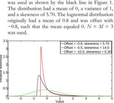
• Non-normal distribution. A lognormal distribution was used as shown by the black line in Figure 1. The distribution had a mean of 0, a variance of 1, and a skewness of 5.70. The lognormal distribution originally had a mean of 0.8 and was offset with
−0.8, such that the mean equaled 0. N = M = 3 was used.
Figure 1. Probability density function of the investigated non-normal distributions (mean = 0, variance = 1).
Furthermore, it was investigated whether other types of tests improve the statistical power and the false positive rate. Specifically, this study evaluated (a) the t-test on ranked data (t-testR) and (b) the t-test using the assumption that the two samples come from normal distributions with unknown and unequal variances, also known as the Welch test. The degrees of freedom for the Welch test was determined with the Welch-Satterthwaite equation (Satterthwaite, 1946). The t-testR was implemented by concatenating the two samples into one vector, applying a rank transformation on this vector, splitting the vector, and then submitting the two vectors with ranked data to the two-sample t-test. This approach gives p values that are highly similar to, and a monotonic increasing function of, the p values obtained with the Mann-Whitney-Wilcoxon test (Conover & Iman, 1981; Zimmerman & Zumbo, 1989, 1993). Note that when sample sizes are extremely small, the Mann-Whitney-Wilcoxon test is somewhat more conservative (i.e., provides higher p values) than the t-testR.
An additional analysis was performed to explore how the Type I error rate and statistical power vary as a function of the degree of skewness of the lognormal distribution. The offset value (originally −0.8) of the
-3 -2 -1 0 1 2 3 4 5 0 0.5 1 1.5 2 2.5 3 3.5 Value Relat iv e lik elihood Offset = -0.8, skewness = 5.70 Offset = -0.5, skewness = 14.0 Offset = -10.0, skewness = 0.30
population distribution was systematically varied with 20 logarithmically spaced values between −0.1 and
−100, while holding the population mean at 0 and the population variance at 1. Changing the offset value while holding the mean and variance constant influences skewness (see Figure 1 for an illustration). D = 0 was used for estimating the Type I error rate and D = 2 was used for estimating the Type II error rate.
Finally, the paired t-test was evaluated. This study investigated its behavior for N = 3 as a function of the within-pair population correlation coefficient (r). The correlation coefficient was varied between −0.99 and 0.99.
The analyses were conducted in MATLAB (Version R2010b, The MathWorks, Inc., Natick, MA). The MATLAB code for the simulations is provided in the appendix, and may be used for testing the effect of the simulation parameters such as sample size or parameters of the non-normal distribution.
Results
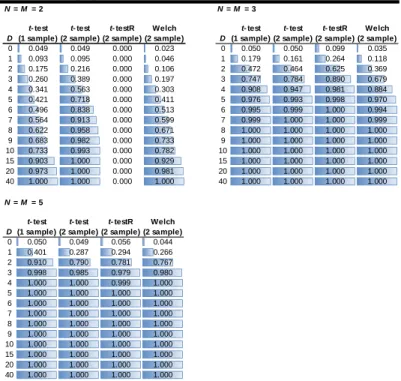
The results for equal sample sizes (N = M = 2, N = M = 3, & N = M = 5) are shown in Table 1. For the one-sample t-test, acceptable statistical power (i.e., 1 – beta > 80%) is reached for D ≥ 12. For the two-sample t-test, acceptable power is reached for D ≥ 6. In other words, the t-test provides acceptable power for extremely small sample sizes, provided that the population effect size is very large. Table 1 further shows that the t-testR has zero power for any effect size when N = M = 2. The results in Table 2 also reveal that the Welch t-test is not preferred; statistical power is lower as compared to the regular t-test.
For N = M = 3, the null hypothesis is rejected in more than 80% of the one-sample and two-sample t -tests for D ≥ 4 (Table 1). The t-testR provides a power advantage as compared to the t-test. However, the Type I error rate of the t-testR is 9.9%, which is substantially higher than the nominal value of 5%. Again, the Welch test results in diminished statistical power as compared to the regular t-test.
For N = M = 5, the statistical power is 91.0% and 79.0% at D = 2, for the one-sample and two-sample t -test, respectively. For this sample size, the power differences between the t-test, t-testR, and Welch test
are small, and either test might be chosen. The Type I error rates of the regular t-test are close to the nominal level of 5% for all four t-test variants (Table 1).
Table 1. Proportion of 100,000 repetitions yielding p < 0.05
for various mean distances D. The simulations were
conducted with equal sample sizes per group and normally distributed populations.
Note: The values for D= 0 represent the Type I error rate. The values for D > 0 represent statistical power (i.e., 1−Type II error rate).
Table 2 shows the results for extremely small and unequal sample sizes (i.e., N = 2, M = 5). The t-test and t-testR provide more than 80% power for D ≥ 3. The t-testR yields a high Type I error rate of 9.4%. The Welch test provides diminished power as compared to the regular t-test.
Table 2 further shows the results for unequal variances for N = M = 3. The t-testR provides greater statistical power than the t-test (cf. 72.9% for t-testR vs. 52.9% for the t-test at D = 3), but yields a high Type I error rate of 15.7%. The Welch test again reduces statistical power as compared to the t-test. The Welch test yields an acceptable Type I error rate of 5.5%, that is, slightly above the nominal level of 5.0%, whereas for the regular t-test the false positive rate is 8.3%.
N = M = 2 N = M = 3 D t- test (1 sample) t- test (2 sample) t- testR (2 sample) Welch (2 sample) D t- test (1 sample) t- test (2 sample) t- testR (2 sample) Welch (2 sample) 0 0.049 0.049 0.000 0.023 0 0.050 0.050 0.099 0.035 1 0.093 0.095 0.000 0.046 1 0.179 0.161 0.264 0.118 2 0.175 0.216 0.000 0.106 2 0.472 0.464 0.625 0.369 3 0.260 0.389 0.000 0.197 3 0.747 0.784 0.890 0.679 4 0.341 0.563 0.000 0.303 4 0.908 0.947 0.981 0.884 5 0.421 0.718 0.000 0.411 5 0.976 0.993 0.998 0.970 6 0.496 0.838 0.000 0.513 6 0.995 0.999 1.000 0.994 7 0.564 0.913 0.000 0.599 7 0.999 1.000 1.000 0.999 8 0.622 0.958 0.000 0.671 8 1.000 1.000 1.000 1.000 9 0.683 0.982 0.000 0.733 9 1.000 1.000 1.000 1.000 10 0.733 0.993 0.000 0.782 10 1.000 1.000 1.000 1.000 15 0.903 1.000 0.000 0.929 15 1.000 1.000 1.000 1.000 20 0.973 1.000 0.000 0.981 20 1.000 1.000 1.000 1.000 40 1.000 1.000 0.000 1.000 40 1.000 1.000 1.000 1.000 N = M = 5 D t- test (1 sample) t- test (2 sample) t- testR (2 sample) Welch (2 sample) 0 0.050 0.049 0.056 0.044 1 0.401 0.287 0.294 0.266 2 0.910 0.790 0.781 0.767 3 0.998 0.985 0.979 0.980 4 1.000 1.000 0.999 1.000 5 1.000 1.000 1.000 1.000 6 1.000 1.000 1.000 1.000 7 1.000 1.000 1.000 1.000 8 1.000 1.000 1.000 1.000 9 1.000 1.000 1.000 1.000 10 1.000 1.000 1.000 1.000 15 1.000 1.000 1.000 1.000 20 1.000 1.000 1.000 1.000 40 1.000 1.000 1.000 1.000
Table 2. Proportion of 100,000 repetitions yielding p < 0.05
for various mean distances D. The simulations were
conducted with normally distributed populations having unequal sample sizes (left pane) and unequal variances (right pane).
Note: The values for D = 0 represent the Type I error rate. The values for D > 0 represent statistical power (i.e., 1−Type II error rate).
For unequal sample sizes and unequal variances, a mixed picture arises (Table 3). When the larger sample is drawn from the high variance population, the t-testR and the Welch test are preferred over the regular t-test, because the statistical power is higher for these two tests. However, when the larger sample is drawn from the low variance population, none of the three statistical tests can be recommended. The t-test and t -testR provide unacceptably high false positive rates (> 27%), whereas the Welch test provides very low power: even for an effect as large as D = 20, the statistical power is only 76.5%. The high Type I error rate for the t-test is caused by the fact that the pooled standard deviation is determined mostly by the larger sample (having the lower variability), while the difference in sample means is determined mostly by the smaller sample (having the higher variability). As a result, the t -statistic is inflated.
Table 4 shows that for a lognormal distribution, the t-testR provides the greatest statistical power. For example, for D = 1, the power is 57.4%, 39.8%, and 30.4%, for the t-testR, regular t-test, and Welch test, respectively. However, the Type I error rate is high for the t-testR (9.9%) as compared to the regular t-test (3.4%) and the Welch test (2.0%). The Type I error rate of the one-sample t-test is very high (15.3%). Note that for larger sample sizes (i.e., N = M = 15), the t-testR provides an accurate Type I error rate of 5%, while the
one-sample t-test retains a high Type I error rate of 13.9% (data not shown).
Table 3. Proportion of 100,000 repetitions yielding p < 0.05
for various mean distances D. The simulations were
conducted with normally distributed populations having unequal sample sizes combined with unequal variances.
Note: The values for D = 0 represent the Type I error rate. The values for D > 0 represent statistical power (i.e., 1−Type II error rate).
Table 4. Proportion of 100,000 repetitions yielding p < 0.05
for various mean distances D. The simulations were
conducted for the lognormal distribution shown in Figure 1 (skewness = 5.70) with equal sample sizes per group.
Note: The values for D= 0 represent the Type I error rate. The values for D > 0 represent statistical power (i.e., 1−Type II error rate).
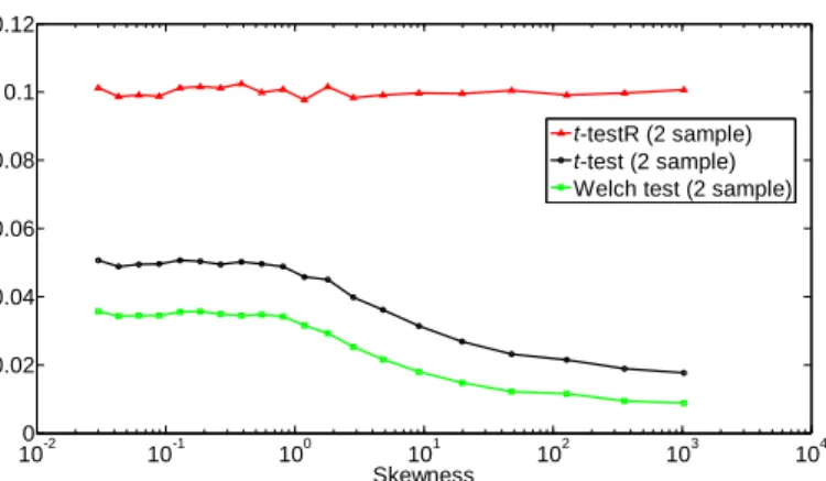
Figures 2 and 3 present the results of the simulations for the 20 different degrees of skewness (N = M = 3). It can be seen that Type I error rates are relatively independent of the degree of skewness (Figure 2). Statistical power at D = 2 increases with increasing skewness (Figure 3). This phenomenon can be explained by the fact that the probability that the tail of the distribution is sampled is small when skewness is
N = 2, M = 5 N = M = 3 (unequal variances) D t- test (2 sample) t- testR (2 sample) Welch (2 sample) D t- test (2 sample) t- testR (2 sample) Welch (2 sample) 0 0.050 0.094 0.063 0 0.083 0.157 0.055 1 0.162 0.252 0.165 1 0.148 0.255 0.098 2 0.487 0.609 0.384 2 0.314 0.487 0.210 3 0.816 0.885 0.559 3 0.529 0.729 0.362 4 0.963 0.980 0.654 4 0.723 0.887 0.516 5 0.996 0.998 0.722 5 0.858 0.963 0.662 6 1.000 1.000 0.770 6 0.939 0.991 0.774 7 1.000 1.000 0.813 7 0.978 0.998 0.861 8 1.000 1.000 0.846 8 0.993 1.000 0.920 9 1.000 1.000 0.874 9 0.998 1.000 0.957 10 1.000 1.000 0.897 10 1.000 1.000 0.977 15 1.000 1.000 0.966 15 1.000 1.000 1.000 20 1.000 1.000 0.991 20 1.000 1.000 1.000 40 1.000 1.000 1.000 40 1.000 1.000 1.000
N = 2 (small variance), M = 5 (large variance) N = 5 (small variance), M = 2 (large variance)
D t- test (2 sample) t- testR (2 sample) Welch (2 sample) D t- test (2 sample) t- testR (2 sample) Welch (2 sample) 0 0.014 0.046 0.041 0 0.271 0.309 0.104 1 0.043 0.122 0.117 1 0.352 0.392 0.126 2 0.154 0.345 0.350 2 0.547 0.587 0.176 3 0.354 0.627 0.652 3 0.748 0.785 0.232 4 0.598 0.844 0.874 4 0.883 0.910 0.279 5 0.801 0.949 0.966 5 0.955 0.971 0.323 6 0.922 0.988 0.992 6 0.986 0.993 0.360 7 0.976 0.998 0.997 7 0.995 0.998 0.397 8 0.994 1.000 0.999 8 0.999 1.000 0.432 9 0.999 1.000 0.999 9 1.000 1.000 0.464 10 1.000 1.000 1.000 10 1.000 1.000 0.494 15 1.000 1.000 1.000 15 1.000 1.000 0.645 20 1.000 1.000 1.000 20 1.000 1.000 0.765 40 1.000 1.000 1.000 40 1.000 1.000 0.977 N = M = 3 (lognormal) D t- test (1 sample) t- test (2 sample) t- testR (2 sample) Welch (2 sample) 0 0.153 0.034 0.099 0.020 1 0.332 0.398 0.574 0.304 2 0.783 0.728 0.830 0.626 3 0.907 0.867 0.922 0.789 4 0.952 0.929 0.960 0.872 5 0.972 0.959 0.978 0.917 6 0.984 0.975 0.987 0.945 7 0.989 0.984 0.991 0.961 8 0.992 0.989 0.995 0.973 9 0.995 0.992 0.996 0.979 10 0.996 0.994 0.997 0.984 15 0.999 0.999 0.999 0.995 20 1.000 1.000 1.000 0.998 40 1.000 1.000 1.000 1.000
high. In other words, for high skewness (cf. red line in Figure 1) the sample distribution is often narrow, and consequently, shifting one of the samples with D = 2 results in a high t-statistic and low p value. For all degrees of skewness, the t-testR retains a higher Type I error rate (Figure 2) and greater statistical power (Figure 3) than the t-test and Welch test.
Figure 2. Type I error rate of the two-sample t-test, the
two-sample t-test after rank transformation (t-testR), and the
Welch test, as a function of the degree of skewness of the
lognormal distribution (N = M = 3).
Figure 3. Statistical power at D = 2 of the two-sample t-test,
the two-sample t-test after rank transformation (t-testR), and
the Welch test, as a function of the degree of skewness of
the lognormal distribution (N = M = 3).
Figure 4 shows the results of the paired t-test. It can be seen that statistical power improves when the within-pair correlation increases. Acceptable statistical power (> 80%) can be obtained with N = 3, as long as the within-pair correlation is high (r > 0.8). A negative correlation diminishes statistical power, which can be explained by the fact that the variance of the paired
differences increases when the correlation coefficient decreases. The results in Figure 4 are in agreement with the statement that “in rare cases, the data may be negatively correlated within subjects, in which case the unpaired test becomes anti-conservative” (Wikipedia, 2013; cf. 46.4% and 62.5% statistical power for the unpaired t-test and t-testR at N = M = 3, Table 1). Figure 4 further illustrates that the Type I error rate is again higher for the t-testR as compared to the regular t-test.
Figure 4. Type I error rate and statistical power (1-Type II
error rate) for the paired t-test as a function of the
within-pair correlation coefficient (r). Simulations were conducted
with N = 3. D = 0 was used for estimating the Type I error
rate and D = 2 was used for estimating the statistical power.
Discussion
The present simulation study showed that there is no fundamental objection to using a regular t-test with extremely small sample sizes. Even a sample size as small as 2 did not pose problems. In most of the simulated cases, the Type I error rate did not exceed the nominal value of 5%. A paired t-test is also feasible with extremely small sample sizes, particularly when the within-pair correlation coefficient is high.
A high Type I error rate was observed for unequal variances combined with unequal sample sizes (with the smaller sample drawn from the high variance population), and for a one-sample t-test applied to non-normally distributed data. The simulations further clarified that when the sample size is extremely small, Type II errors can only be avoided if the effect size is extremely large. In other words, conducting a t-test
10-2 10-1 100 101 102 103 104 0 0.02 0.04 0.06 0.08 0.1 0.12 Skewness T y p e I e rro r ra te t-testR (2 sample) t-test (2 sample) Welch test (2 sample)
10-2 10-1 100 101 102 103 104 0.4 0.5 0.6 0.7 0.8 0.9 1 Skewness Statis tic a l pow er a t D = 2 t-testR (2 sample) t-test (2 sample) Welch test (2 sample)
-1 -0.8 -0.6 -0.4 -0.2 0 0.2 0.4 0.6 0.8 1 0 0.2 0.4 0.6 0.8 1 r Ty pe I err o r rate / S ta ti s ti c a l powe r at D
= 2 Type I error rate t-test Type I error rate t-testR 1-Type II error rate t-test 1-Type II error rate t-testR
with extremely small samples is feasible, as long as the true effect size is large.
The fact that the t-test functions properly for extremely small sample sizes may come as no surprise to the informed reader. In fact, William Sealy Gosset (working under the pen name “Student”) developed the t-test especially for small sample sizes (Student, 1908; for reviews see Box, 1987; Lehmann, 2012; Welch, 1958; Zabell, 2008), a condition where the traditional z -test provides a high rate of false positives. Student himself verified his t-distribution on anthropometric data of 3,000 criminals, which he randomly divided into 750 samples each having a sample size of 4.
The simulations showed that a rank transformation is not recommended when working with extremely small sample sizes. Although the t-testR occasionally improved statistical power with respect to the regular t-test, the Type I error rate was disproportionally high in most of the investigated cases. However, for N = M = 2, application of the rank transformation resulted in 0% Type I errors and 100% Type II errors. The erratic Type I/II error behavior of the t-testR can be explained by a quantization phenomenon, as also explained by Janušonis (2009). There are (2N)!/(N!*N!) ways to distribute 2N cases into two groups (Sloane, 2003, sequence A000984), setting an upper limit to the number of possible differences in mean ranks, being ceil(N^2+1)/2) (Sloane, 2003; sequence A080827). For N = M = 2, three distinct p values are possible (i.e., 0.106, 0.553, & 1.000). Illustratively, if submitting the following two vectors to the two-sample t-test: [1 2] and [3 4], the resulting p value is 0.106, so even in this ‘perfectly ordered’ condition the null hypothesis will not be rejected. For N = M = 3, five distinct p values are possible (0.021, 0.135, 0.326, 0.573, & 0.854), for N = M = 4, nine distinct p values are possible, and for N = M = 5, 13 different p values can be obtained. Some researchers have recommended rank-based tests when working with highly skewed distributions (e.g., Bridge & Sawilowsky, 1999). The present results showed that a rank-transformation is not to be preferred when working with extremely small sample sizes, because of quantization issues.
The t-test with the unequal variances option (i.e., the Welch test) was generally not preferred either. Only in the case of unequal variances combined with unequal sample sizes, where the small sample was drawn from the small variance population, did this approach provide a power advantage compared to the regular t -test. In the other cases, a substantial amount of statistical power was lost compared to the regular t-test. The power loss of the Welch test can be explained by its lower degrees of freedom determined from the Welch-Satterthwaite equation. For N = M = 2, and normally distributed populations with equal variances, the degrees of freedom of the Welch test is on average 1.41, compared to 2.0 for the t-test. To the credit of the Welch test, the Type I error rates never deviated far from the nominal 5% value, and were in several cases substantially below 5%. Similar results for unequal sample sizes (Ns between 6 and 25) and unequal variances were reported in a review article about the Welch test by Ruxton (2006).
Some researchers have recommended that when sample sizes are small, a permutation test (also called exact test or randomization test) should be used instead of a t-test (e.g., Ludbrook & Dudley, 1998). In a follow-up analysis, I repeated the two-sample comparisons by means of a permutation test using the method described by Hesterberg et al. (2005). The permutation test yielded Type I and Type II error rates that were similar to the t-testR. This similarity can be explained by the fact that for extremely small sample sizes, a permutation test suffers from a similar quantization problem as the t-testR. A permutation test may be useful for analyzing data sampled from a highly skewed distribution. However, permutation tests or other resampling techniques, such as bootstrapping and jackknifing, do not overcome the weakness of small samples in statistical inference (Hesterberg et al., 2005).
This study showed that there are no objections to using a t-test with extremely small samples, as long as the effect size is large. For example, researchers can safely use a group size of only 3 when D = 6 or larger and the population distribution is normal. Such large effects may be quite common in engineering and physical sciences where variability and measurement error tend to be small. However, large effect sizes are uncommon in the behavioral/psychological sciences.
Bem et al. (2011) and Richard et al. (2003) stated that effect sizes in psychology typically fall in the range of 0.2 to 0.3. In some cases, large effects do occur in behavioral research. For example, severe and enduring early isolation may have strong permanent effects on subsequent behavior and social interaction (see Harlow et al., 1965 for a study on monkeys), strong physical stimuli—particularly electric shock and warmth—are perceived as highly intensive (Stevens, 1961), and training/practice can dramatically alter skilled performance. Shea and Wulf (1999), for example, found that the angular root mean square error on a task requiring participants to balance on a stabilometer improved with about D = 6 after 21 practice trials. Aging/maturation can also have large effects. Tucker-Drob (2013) mentioned Ds of about 7 for differences in reading, writing, and mathematics skills between 4-year olds and 18-4-year olds. Royle et al. (in press) reported a difference of D = 6 between total brain volume of 18−28-year olds and 84−96-year olds, a biological factor which may explain the age-related decline typically observed in the mean test scores of cognitive abilities such as reasoning, memory, processing speed, and spatial ability. Mesholam et al. (1998) reported large effect sizes (Ds up to 4) on olfactory recognition measures for Alzheimer’s and Parkinson’s disease groups relative to controls. A worldwide study comparing 15-year-old school pupils’ performance on mathematics, reading, and science found differences up to D = 2.5 between countries (OECD, 2010). Mathes et al. (2002) found large sex differences (D = 10.4) on a paper-and-pencil measure of desire for promiscuous sex for respondents in their teens (data reviewed by Voracek et al., 2006). In summary, large effects do occur in the behavioral/psychological sciences.
A final cautionary note is in place. In this work, a frequentist statistical perspective was used. From a Bayesian perspective, small sample sizes may still be problematic and may contribute to false positives and inflated effect sizes (Ingre, in press; Ioannidis, 2005, 2008). This can be explained as follows. In reality, the applied researcher does not know whether the null hypothesis is true or not. It may be possible, however, to estimate the probability that an effect is true or false, based on a literature study of the research field.
Suppose that there is a 50% probability that the null hypothesis is true and a 50% probability that the null hypothesis is false with D = 1. If sample sizes are small, then statistical power is low. For example, if N = M = 2, the probability of a true positive is only 4.7% (9.5% power value in Table 1 * 50%) and the probability of a false positive equals 2.5% (alpha level of 5% * 50%). This implies that the probability that a statistically significant finding reflects a true effect is 65% (i.e., 4.7%/(4.7%+2.5%). Now suppose one uses N = M = 100. The probability of a true positive is now 50% (~100% statistical power * 50%) and the probability of a false positive is still 2.5%, meaning that the positive predictive value is 95%. In other words, when the sample size is smaller, a statistically significant finding is more likely to be a false positive. Taking this further, it can be argued that if a psychologist observes a statistically significant effect based on an extremely small sample size, it is probably grossly inflated with respect to the true effect, because effect sizes in psychological research are typically small. Accordingly, researchers should always do a comprehensive literature study, think critically, and investigate whether their results are credible in line with existing evidence in the research field.
Summarizing, given infinite time and resources, large samples are always preferred over small samples. Should the applied researcher conduct research with an extremely small sample size (N ≤ 5), the t-test can be applied, as long as the effect size is expected to be large. Also in case of unequal variances, unequal sample sizes, or skewed population distributions, can the t-test be validly applied in an extremely-small-sample scenario (but beware the high false positive rate of the one-sample t-test on non-normal data, and the high false positive rate that may occur for unequal sample sizes combined with unequal variances). A rank-transformation and the Welch test are generally not recommended when working with extremely small samples. Finally, researchers should always judge the credibility of their findings and should remember that extraordinary claims require extraordinary evidence.
References
Bem, D. J., Utts, J., & Johnson, W. O. (2011). Must psychologists change the way they analyze their data?
Journal of Personality and Social Psychology, 101, 716–719. Blair, R. C., Higgins, J. J., & Smitley, W. D. (1980). On the
relative power of the U and t tests. British Journal of
Mathematical and Statistical Psychology, 33, 114–120. Box, J. F. (1987). Guinness, Gosset, Fisher, and small
samples. Statistical Science, 2, 45–52.
Bridge, P. D., & Sawilowsky, S. S. (1999). Increasing physicians’ awareness of the impact of statistics on research outcomes: comparative power of the t-test and Wilcoxon rank-sum test in small samples applied
research. Journal of Clinical Epidemiology, 52, 229–235.
Campbell, M. J., Julious, S. A., & Altman, D. G. (1995). Estimating sample sizes for binary, ordered categorical, and continuous outcomes in two group comparisons.
BMJ: British Medical Journal, 311, 1145–1148. Cohen, J. (1970). Approximate power and sample size
determination for common one-sample and
two-sample hypothesis tests. Educational and Psychological
Measurement, 30, 811–831.
Conover, W. J., & Iman, R. L. (1981). Rank transformations as a bridge between parametric and nonparametric
statistics. The American Statistician, 35, 124–129.
De Winter, J. C. F., & Dodou, D. (2010). Five-point Likert
items: t test versus Mann-Whitney-Wilcoxon. Practical
Assessment, Research & Evaluation, 15, 11.
Elliott, A. C., & Woodward, W. A. (2007). Comparing one or
two means using the t-test. Statistical Analysis Quick Reference Guidebook. SAGE.
Fay, M. P., & Proschan, M. A. (2010).
Wilcoxon-Mann-Whitney or t-test? On assumptions for hypothesis tests
and multiple interpretations of decision rules. Statistics
Surveys, 4, 1–39.
Fitts, D. A. (2010). Improved stopping rules for the design of efficient small-sample experiments in biomedical and
biobehavioral research. Behavior Research Methods, 42, 3–
22.
Fritz, C. O., Morris, P. E., & Richler, J. J. (2012). Effect size estimates: Current use, calculations, and interpretation.
Journal of Experimental Psychology: General, 141, 2–18. Harlow, H. F., Dodsworth, R. O., & Harlow, M. K. (1965).
Total social isolation in monkeys. Proceedings of the
National Academy of Sciences of the United States of America,
54, 90–97.
Hesterberg, T., Moore, D. S., Monaghan, S., Clipson, A., & Epstein, R. (2005). Bootstrap methods and permutation tests. Introduction to the Practice of Statistics, 5, 1–70. Ingre, M. (in press). Why small low-powered studies are
worse than large high-powered studies and how to protect against “trivial” findings in research: Comment
on Friston (2012). NeuroImage.
Ioannidis, J. P. (2005). Why most published research
findings are false. PLOS Medicine, 2, e124.
Ioannidis, J. P. (2008). Why most discovered true
associations are inflated. Epidemiology, 19, 640–648.
Ioannidis, J. P. (2013). Mega-trials for blockbusters. JAMA,
309, 239–240.
Janušonis, S. (2009). Comparing two small samples with an
unstable, treatment-independent baseline. Journal of
Neuroscience Methods, 179, 173–178.
Lehmann, E. L. (2012). “Student” and small-sample theory. In
Selected Works of E.L. Lehmann (pp. 1001–1008). Springer US.
Ludbrook, J., & Dudley, H. (1998). Why permutation tests
are superior to t and F tests in biomedical research. The
American Statistician, 52, 127–132.
Mathes, E.W., King, C.A., Miller, J.K. and Reed, R.M. (2002). An evolutionary perspective on the interaction of age and sex differences in short-term sexual
strategies. Psychological Reports, 90, 949–956.
Mesholam, R. I., Moberg, P. J., Mahr, R. N., & Doty, R. L. (1998). Olfaction in neurodegenerative disease: a meta-analysis of olfactory functioning in Alzheimer’s and
Parkinson’s diseases. Archives of Neurology, 55, 84–90.
Mudge, J. F., Baker, L. F., Edge, C. B., & Houlahan, J. E.
(2012). Setting an optimal α that minimizes errors in
null hypothesis significance tests. PLOS One, 7, e32734.
OECD (2010), PISA 2009 Results: What students know and can do – Student performance in reading, mathematics and science (volume I)
http://dx.doi.org/10.1787/9789264091450-en
Pashler, H., & Harris, C. R. (2012). Is the replicability crisis
overblown? Three arguments examined. Perspectives on
Psychological Science, 7, 531–536.
Posten, H. O. (1982). Two-sample Wilcoxon power over the
Pearson system and comparison with the t-test. Journal
of Statistical Computation and Simulation, 16, 1–18. Ramsey, P. H. (1980). Exact Type 1 error rates for
robustness of Student’s t test with unequal variances.
Richard, F. D., Bond, C. F., Jr., & Stokes-Zoota, J. J. (2003). One hundred years of social psychology quantitatively
described. Review of General Psychology, 7, 331–363.
Rossi, J. S. (1990). Statistical power of psychological
research: What have we gained in 20 years? Journal of
Consulting and Clinical Psychology, 58, 646–656.
Rost, D. H. (1991). Effect strength vs. statistical significance: A warning against the danger of small samples: A comment on Gefferth and Herskovits’s article “Leisure
activities as predictors of giftedness”. European Journal
for High Ability, 2, 236–243.
Royle, N. A., Booth, T., Valdés Hernández, M. C., Penke, L., Murray, C., Gow, A. J., ... & Wardlaw, J. M. (in press). Estimated maximal and current brain volume predict cognitive ability in old age. Neurobiology of Aging. Ruthsatz, J., & Urbach, J. B. (2012). Child prodigy: A novel
cognitive profile places elevated general intelligence, exceptional working memory and attention to detail at
the root of prodigiousness. Intelligence, 40, 419–426.
Ruxton, G. D. (2006). The unequal variance t-test is an
underused alternative to Student’s t-test and the Mann–
Whitney U test. Behavioral Ecology, 17, 688–690.
Satterthwaite, F. E. (1946). An approximate distribution of
estimates of variance components. Biometrics Bulletin, 2,
110–114.
Sawilowsky, S. S., & Blair, R. C. (1992). A more realistic look at the robustness and Type II error properties of the t test to departures from population normality.
Psychological Bulletin, 111, 352–360.
Shea, C. H., & Wulf, G. (1999). Enhancing motor learning through external-focus instructions and feedback.
Human Movement Science, 18, 553–571.
Sheppard, C. R. (1999). How large should my sample be? Some quick guides to sample size and the power of
tests. Marine Pollution Bulletin, 38, 439–447.
Siegel, S. (1956). Nonparametric statistics for the behavioral sciences. New York: McGraw-Hill.
Siegel, S. (1957). Nonparametric statistics. The American
Statistician, 11, 13–19.
Siegel, S., & Castellan, N. J. (1988). Nonparametric statistics for
the behavioral sciences. Second Edition. New York: McGraw-Hill.
Sloane, N. J. (2003). The on-line encyclopedia of integer sequences. http://oeis.org.
Stevens, S. S. (1961). To honor Fechner and repeal his law.
Science, 133, 80–86.
Student. (1908). The probable error of a mean. Biometrika, 6,
1–25.
Tucker-Drob, E. M. (2013). How many pathways underlie socioeconomic differences in the development of
cognition and achievement? Learning and Individual
Differences, 25, 12–20.
Voracek, M., Fisher, M. L., Hofhansl, A., Vivien Rekkas, P., & Ritthammer, N. (2006). "I find you to be very attractive..." Biases in compliance estimates to sexual
offers. Psicothema, 18, 384–391.
Welch, B. L. (1958), “ ‘Student’ and Small Sample Theory,”
Journal of the American Statistical Association, 53, 777–788 Wikipedia (2013).
http://en.wikipedia.org/wiki/Paired_difference_test
Accessed 21 July 2013.
Zabell, S. L. (2008). On Student’s 1908 article “The
Probable Error of a Mean”. Journal of the American
Statistical Association, 103, 1–7.
Zimmerman, D. W., & Zumbo, B. D. (1989). A note on rank transformations and comparative power of the student t-test and Wilcoxon-Mann-Whitney Test.
Perceptual and Motor Skills, 68, 1139–1146. Zimmerman, D. W., & Zumbo, B. D. (1993). Rank
transformations and the power of the Student t-test and Welch t’ test for non-normal populations with
unequal variances. Canadian Journal of Experimental
Psychology, 47, 523–539.
Appendix
% MATLAB simulation code for producing Figure 1 and Tables 1-4
close all;clear all;clc
m = 0.8;v = 1;mu = log((m^2)/sqrt(v+m^2));sigma = sqrt(log(v/(m^2)+1)); % parameters for lognormal
distribution
DD=[0:1:10 15 20 40];
CC=[2 2 1 1 % 1. equal sample size, equal variance
3 3 1 1 % 2. equal sample size, equal variance
2 5 1 1 % 4. unequal sample size, equal variance
3 3 2 1 % 5. equal sample size, unequal variance
2 5 2 1 % 6. unequal sample size, unequal variance
5 2 2 1 % 7. unequal sample size, unequal variance
3 3 1 2 % 8. equal sample size, equal variance, non-normal distribution
15 15 1 2]; % 9. equal sample size, equal variance, non-normal distribution ("large sample"
verification) reps=100000; p1=NaN(size(CC,1),length(DD),reps); p2=NaN(size(CC,1),length(DD),reps); p3=NaN(size(CC,1),length(DD),reps); p4=NaN(size(CC,1),length(DD),reps); for i3=1:size(CC,1) for i2=1:length(DD)
disp([i3 i2]) % display counter
for i=1:reps
N=CC(i3,1); M=CC(i3,2); R=CC(i3,3);
if CC(i3,4)==1; % normal distribution
X=randn(N,1)/R+DD(i2); % sample with population mean = D
X2=randn(M,1)*R; % sample with population mean = 0
else % non-normal distribution
X=(lognrnd(mu,sigma,N,1)-m)/R+DD(i2); % sample with population mean = D
X2=(lognrnd(mu,sigma,M,1)-m)*R; % sample with population mean = 0
end
V=tiedrank([X;X2]); % rank transformation of concatenated vectors
[~,p1(i3,i2,i)]=ttest(X); % one sample t-test with respect to 0
[~,p2(i3,i2,i)]=ttest2(X,X2); % two sample t-test
[~,p3(i3,i2,i)]=ttest2(V(1:N),V(N+1:end)); % two sample t-test after rank transformation
(t-testR)
[~,p4(i3,i2,i)]=ttest2(X,X2,[],[],'unequal'); % two-sample t-test using unequal variances
option (Welch test)
end
end
end
%% display results of Tables 1-4
for i3=1:size(CC,1)
disp(CC(i3,:,:))
disp([DD' mean(squeeze(p1(i3,:,:))'<.05)' mean(squeeze(p2(i3,:,:))'<.05)' mean(squeeze(p3(i3,:,:))'<.05)' mean(squeeze(p4(i3,:,:))'<.05)'])
end
%% make figure 1
m = 0.8;v = 1;mu = log((m^2)/sqrt(v+m^2));sigma = sqrt(log(v/(m^2)+1)); % parameters for lognormal
distribution, offset = -0.8 H=lognrnd(mu,sigma,1,5*10^7)-m; VEC=-10:.05:20;
DIS=histc(H,VEC);DIS=DIS./sum(DIS)/mean(diff(VEC));
figure;plot(VEC,DIS,'k','Linewidth',3)
m = 0.5;v = 1;mu = log((m^2)/sqrt(v+m^2));sigma = sqrt(log(v/(m^2)+1)); % parameters for lognormal
distribution, offset = -0.5 H=lognrnd(mu,sigma,1,5*10^7)-m;
DIS=histc(H,VEC);DIS=DIS./sum(DIS)/mean(diff(VEC));
hold on;plot(VEC,DIS,'r','Linewidth',3)
m = 10;v = 1;mu = log((m^2)/sqrt(v+m^2));sigma = sqrt(log(v/(m^2)+1)); % parameters for lognormal
distribution, offset = -10.0 H=lognrnd(mu,sigma,1,5*10^7)-m;
DIS=histc(H,VEC);DIS=DIS./sum(DIS)/mean(diff(VEC));
plot(VEC,DIS,'g','Linewidth',3)
xlabel('Value','Fontsize',36,'Fontname','Arial')
ylabel('Relative likelihood','Fontsize',36,'Fontname','Arial')
h = findobj('FontName','Helvetica');
set(h,'FontSize',36,'Fontname','Arial')
legend('Offset = -0.8, skewness = 5.70','Offset = -0.5, skewness = 14.0','Offset = -10.0, skewness
= 0.30') % skewness calculated as: sqrt(exp(sigma^2)-1)*(2+exp(sigma^2))
%% MATLAB simulation code for producing Figure 4
clear all
RR=[-0.99 -0.95:0.05:0.95 0.99]; % vector of within-pair Pearson correlations
DD=[0 2]; reps=100000; p1=NaN(length(DD),length(RR),reps); p2=NaN(length(DD),length(RR),reps); for i3=1:length(DD) for i2=1:length(RR)
disp([i3 i2]) % display counter
for i=1:reps
N=3; M=3; D=DD(i3); r=RR(i2);
X=randn(N,1)+D; % sample with population mean = D
X2=r*(X-D)+sqrt((1-r^2))*randn(M,1); % sample with population mean = 0
V=tiedrank([X;X2]); % rank transformation of combined sample
[~,p1(i3,i2,i)]=ttest(X,X2); % paired t-test
[~,p2(i3,i2,i)]=ttest(V(1:N),V(N+1:end)); % paired t-test after rank transformation
(t-testR)
end
end
end
figure;hold on % make figure 4
plot(RR, mean(squeeze(p1(1,:,:))'<.05)','k-o','Linewidth',3,'MarkerSize',15)
plot(RR, mean(squeeze(p2(1,:,:))'<.05)','k-s','Linewidth',3,'MarkerSize',15)
plot(RR, mean(squeeze(p1(2,:,:))'<.05)','r-o','Linewidth',3,'MarkerSize',15)
plot(RR, mean(squeeze(p2(2,:,:))'<.05)','r-s','Linewidth',3,'MarkerSize',15)
xlabel('\it{r}\rm','FontSize',32,'FontName','Arial')
ylabel('Type I error rate / Statistical power at \it{D}\rm = 2','FontSize',32,'FontName','Arial')
legend('Type I error rate \it{t}\rm-test','Type I error rate \it{t}\rm-testR','1-Type II error rate
\it{t}\rm-test','1-Type II error rate \it{t}\rm-testR',2)
h=findobj('FontName','Helvetica'); set(h,'FontName','Arial','fontsize',32)
Citation:
de Winter, J.C.F.. (2013). Using the Student’s t-test with extremely small sample sizes. Practical Assessment, Research & Evaluation, 18(10). Available online: http://pareonline.net/getvn.asp?v=18&n=10.
Author:
J.C.F. de Winter
Department BioMechanical Engineering
Faculty of Mechanical, Maritime and Materials Engineering Delft University of Technology
Mekelweg 2 2628 CD Delft The Netherlands