The Evolution of Hourly Compensation in Canada between 1980 and 2010

(1)

The Evolution of Hourly Compensation in Canada

between 1980 and 2010

Mémoire

Mathieu Pellerin

Maîtrise en économique Maître ès arts (M.A.)

(2)

(3)

Résumé

Nous étudions l’évolution des salaires horaires au Canada au cours des trois dernières décennies à l’aide de données confidentielles du recensement et de l’Enquête nationale sur les ménages. Nous trouvons que le coefficient de variation des salaires chez les travailleurs à temps plein a presque doublé entre 1980 et 2010. La croissance rapide du 99,9e _{centile est le principal} facteur expliquant cette hausse. Les changements dans la composition de la population active expliquent moins de 25% de la hausse de l’inégalité. Toutefois, des effets de composition expliquent la majorité de la hausse du salaire horaire moyen sur la période, alors que les salaires stagnent pour un niveau de compétence donné.

(4)

(5)

Abstract

We consider changes in the distribution of hourly compensation in Canada over the last three decades using confidential census data and the recent National Household Survey. We find that the coefficient of variation of wages among full-time workers has almost doubled between 1980 and 2010. The rapid growth of the 99.9th_{percentile is the main driver of that increase. Changes} in the composition of the workforce explain less than 25% of the rise in wage inequality. However, composition changes explain most of the increase in average hourly compensation over those three decades, while wages stagnate within skill groups.

(6)

(7)

List of Tables

1.1 Variables and time of measurement in the Census/NHS of year t . . . 6 1.2 Work activity and conditional probability of working full-time in the reference

week, respondents aged 15 and above, 2010-2011 population . . . 7 2.1 Evolution of the hourly wage distribution among full-time workers (2010

con-stant dollars) . . . 11 2.2 Evolution of educational status among full-time workers . . . 13 2.3 Mean hourly compensation among full-time workers, by year and education

(2010 constant dollars) . . . 13 2.4 Coefficient of variation of hourly compensation, by year and education . . . 14 2.5 Evolution of potential experience among full-time workers . . . 15 2.6 Mean hourly compensation among full-time workers, by year and potential

ex-perience (2010 constant dollars) . . . 16 2.7 Coefficient of variation of hourly compensation, by year and potential experience 16 2.8 Evolution of gender among full-time workers. . . 17 2.9 Mean (in 2010 constant dollars) and coefficient of variation of hourly

compen-sation, by year and gender . . . 17 2.10 Mean (in 2010 constant dollars) and coefficient of variation of hourly

compen-sation, by year and immigrant status . . . 18 3.1 Variance decomposition, skill distribution of 1981, wage structure of 2006 . . . 20 3.2 Variance decomposition, skill distribution of 1981, wage structure of 2011 . . . 21 3.3 Variance decomposition, skill distribution of 2006, wage structure of 1981 . . . 21 3.4 Variance decomposition, skill distribution of 2011, wage structure of 1981 . . . 21 3.5 Evolution of the 99th _{percentile of hourly compensation by education group}

(10)

(11)

List of Figures

0.1 Hourly compensation growth, top percentiles . . . 3 2.1 Hourly compensation among full-time workers and real GDP per hour, 1980-2005. 12 3.1 Average hourly compensation among full-time workers, actual and conterfactual

with composition of year B (2010 constant dollars) . . . 23 3.2 Median hourly compensation among full-time workers, actual and conterfactual

with composition of year B (2010 constant dollars) . . . 24 3.3 Hourly compensation among full-time workers, 90th _{percentile, actual and}

con-terfactual with composition of year B (2010 constant dollars) . . . 24 3.4 Hourly compensation among full-time workers, 99th _{percentile, actual and}

con-terfactual with composition of year B (2010 constant dollars) . . . 26 3.5 Hourly compensation among full-time workers, 99.9th _{percentile, actual and}

(12)

(13)

Remerciements

Merci à mon directeur Jean-Yves Duclos, pour m’avoir montré ce qu’un économiste devrait être.

Merci à mon codirecteur Bruce Shearer, pour ses conseils judicieux et l’aide qu’il m’a fournie à un moment crucial pour accélérer la diffusion du manuscrit.

Merci à Philippe Barla, pour sa critique aiguisée (mais toujours juste) dans le cours d’atelier de recherche, qui a permis d’améliorer le présent mémoire considérablement.

Merci à Nicholas-James Clavet, pour avoir partagé son expertise concernant les jeux de données de Statistique Canada avec une infinie patience.

Finalement, merci à ma famille et amis proches, qui ont joué un rôle plus discret mais tout aussi important dans mon parcours de maîtrise. Ils sont ma plus grande richesse.

(14)

(15)

Avant-propos

Le présent mémoire est tiré d’un article rédigé conjointement avec Jean-Yves Duclos. L’article est présentement en circulation en tant que cahier de recherche 8917 de l’IZA, toujours sous le titre «The Evolution of Hourly Compensation in Canada between 1980 and 2010». Le mémoire diffère légèrement du cahier de recherche puisqu’il incorpore les commentaires émis par les rapporteurs d’une revue scientifique de même que ceux des professeurs ayant évalué le dépôt initial. En particulier, plusieurs tests de robustesse ont été ajoutés à la suite de ces commentaires. Une version très similaire au présent mémoire a été soumise à une revue scientifique au début du mois d’août 2015 et est présentement en cours d’évaluation.

Puisque mon mémoire vient d’un article ayant plusieurs auteurs, la contribution de chaque auteur doit être spécifiée en vertu des règles de la Faculté des études supérieures et post-doctorales de l’Université Laval. J’ai réalisé la totalité du travail sur les données, rédigé la première version de l’article au complet et choisi les méthodes de décomposition ayant généré les résultats au cœur de l’article. Monsieur Duclos a fourni un encadrement régulier, validant les nouveaux résultats obtenus presque à chaque semaine, en plus de fournir plusieurs con-seils quant à la mesure de l’inégalité, son champ de spécialisation. Il a également contribué à finaliser l’article afin qu’il atteigne le niveau de qualité nécessaire à sa diffusion.

Finalement, les résultats du mémoire ont été obtenus à partir de données confidentielles ac-cessibles dans un laboratoire du Centre interuniversitaire québécois de statistiques sociales (CIQSS), organisme qui fait lui-même partie du Réseau canadien des Centres de données de recherche, la branche de Statistique Canada permettant aux chercheurs d’accéder à des jeux de données confidentiels. En ce qui a trait au financement, j’ai reçu des bourses du Conseil de recherches en sciences humaines du Canada, du Fonds de recherche du Québec - Société et culture, de la Chaire de recherche Industrielle Alliance sur les enjeux économiques des change-ments démographiques, de même qu’une bourse du CIQSS. Les opinions et analyses présentées au sein du mémoire n’engagent en rien les organismes susmentionnés.

(16)

(17)

Introduction

This paper quantifies the contribution of changes in the composition of the workforce to the rise of wage inequality in Canada between 1980 and 2010. Several recent studies have documented a significant rise in inequality over that period. For instance, the Gini coefficient of market income estimated on the basis of survey data has risen by 18% between 1976 and 2009 (Figure 1,Fortin et al.,2012). Using tax data,Veall (2012) finds that the income share of the top 1% has increased from 8% to 12% between 1980 and 2010. Although the observable characteristics of the Canadian labour force have changed significantly in the last 30 years, to the best of our knowledge, no study has attempted to determine if composition effects have had a meaningful role in the rise of inequality. This is the main objective of the paper.

Composition effects can increase inequality in at least two ways. Firstly, composition effects may increase the demographic weight of worker categories with higher within-group inequality. Lemieux (2006) finds that within-group inequality is systematically higher among educated and experienced workers in the US. Furthermore, average years of schooling and experience in the US labour force have increased substantially between 1973 and 2003. The resulting composition effects explain between 28% and 75% of the rise in residual inequality 1 _among

American women (between 44% and 70% among men) (Tables 1A and 1B, Lemieux, 2006). Since similar demographic changes have occurred in Canada, composition shifts towards skill groups with higher within-group inequality should have affected inequality in Canada as well. Secondly, a rise in the dispersion of observable characteristics increases the inequality of wages, unless there is a corresponding fall in skill differentials. In 1980, 58% of full-time workers had a high school degree or less and only 13% had a college degree. By contrast, the majority of workers in 2005 had some education beyond high school, and there were approximately as many workers with a college degree (24.2%) as workers with only a high school degree (24.6%). Since the return to education has remained high (and has even increased between 1980 and 2005 — Boudarbat et al. (2010)), this higher dispersion of educational attainments should explain part of the increase in inequality.

1

Suppose that the population is divided in skill groups A and B. Total variance equals V ar[Y] =

E[V ar[Y|X]] + V ar[E[Y|X]], where X ∈ {A, B}. We use the term "residual inequality" to refer to

(18)

When the composition of the workforce is held constant, changes in the wage structure can affect inequality through changes in skill differentials, such as the return to schooling, or through changes in within-group variances, giving us four sources of variation for inequality. In order to quantify the relative importance of these four mechanisms, we use confidential data from the Census of Canada compulsory long form between 1980 and 2005 as well as confidential data from the new National Household Survey. Confidential census data contain several key demographic indicators and measures of income for 20% of the Canadian population, with a new sample available every 5 years. We use hourly compensation to measure inequality and restrict our sample to full-time workers. Measurement issues arise in the construction of our data since the Census does not report hourly compensation directly. In Section1, we argue that census data measure hourly compensation adequately for full-time workers and that our restricted sample yields valuable insights into the evolution of inequality.

The National Household Survey contains the same information as previous censuses, and has a large sample size as well : the main difference is that the NHS is not compulsory and is thus more vulnerable to non-response bias. In spite of this caveat, the results we obtain from NHS data are consistent with other data sources, and our conclusions remain the same whether we use the 2006 census or the 2011 NHS as the last year of our analysis.

We define composition as a vector of four characteristics : education, experience, gender and immigrant status. Using a simple variance decomposition, we find that between 73% and 87% of the rise in inequality can be explained by a considerable expansion of within-group variances rather than composition effects or changes in skill prices. The increase of within-group variances is itself driven by the rapid growth of hourly compensation in the top 0.1%, as observed in Figure0.1. Conterfactual scenarios based on the DFL method (DiNardo et al., 1996) confirm that composition effects do not fully account for the rise of top wages.

However, composition effects have had an important impact on the evolution ofaverage hourly compensation over the period. Average hourly compensation grew by 15.5 percent in our sample between 1980 and 2010, well behind the 39.8 percent growth of GDP per hour worked. This weak performance masks an even more sluggish (sometimes negative) growth within skill groups. When holding the composition of the workforce constant, we find that average hourly compensation falls by 1% to 8% during the period. We obtain similar results when repeating the procedure with the 50th_{, 90}th _{and 99}th _percentiles.

The main contribution of our paper to the litterature is to show that a few key variables account for a large part of the evolution of hourly compensation between 1980 and 2010, except for the highest percentiles of the distribution. We consider our work to be complimentary to studies looking at the evolution of inequality at a more disaggregated level (Fortin and Lemieux,2015), investigating the presence of polarization in the labour market (Green and Sand, 2015), or documenting the occupation and industry of top income earners (Lemieux and Riddell,2015).

(19)

Figure 0.1: Hourly compensation growth, top percentiles

Our findings do not fit neatly in a typical skill-biased technological change narrative, since sluggish wage growth has affected all worker categories, save a tiny minority at the top. This does not mean that technology has not affected wage growth, however. According to Karabar-bounis and Neiman (2014), the slow growth of labour income is a worldwide phenomenon, and is partly caused by a decline in the relative price of investment goods, that might itself be caused by technological advances in the information technology sector. Although this expla-nation remains tentative, it is hard to think of competing explaexpla-nations based on institutions or country-specific trends that would explain the slow growth of wages in a convincing fashion. The surge in top wages is more complex to explain, and we remain agnostic on the issue. The rest of the paper is organized as follows. Chapter 1defines the population we study, ad-dresses issues related to the National Household Survey, and explains how we calculate hourly compensation. Chapter 2 shows the evolution of hourly compensation by education, gen-der, immigrant status and potential experience. Chapter 3 presents the main decomposition results.

(20)

(21)

Chapter 1

Data sources

1.1 Measurement of income in the Canadian census

The Census of Canada is conducted every five years. Up to the 2006 census, 20% of Canadian households received form 2B, known as the long form. The form contained detailed questions about housing, income, language, ethnicity, schooling and a host of other indicators. Since filling the long form was mandatory, census data suffered little from sample selection bias. Starting with the 2011 census, the long form was abolished, a move that sparked controversy (Green and Milligan, 2010; Veall, 2010). Instead, 4.5 million households (about 30% of all private dwellings) received the National Household Survey (NHS) questionnaire; responding was optional, and the unweighted response rate was 68.6% (Statistics Canada,2011b). Previ-ous studies comparing census and voluntary survey data find that low and high incomes are usually underrepresented in surveys, such as the Survey of Consumer Finances (SCF) and the Survey of Labour and Income Dynamics (SLID) (Frenette et al.,2004;Frenette et al.,2007). Since filling the NHS is voluntary, it is susceptible to such biases as well.

However, there are reasons to believe that NHS data may be more reliable than those of the SCF/SLID. Firstly, in order to attenuate non-response bias, Statistics Canada enumerators contacted 400,000 of the 1,200,000 non-respondents in the first wave of the survey to collect their answers (Statistics Canada,2011b). Secondly, the results we obtain from NHS data, such as a slight decline of top wages between 2005 and 2010, are consistent with results obtained from fiscal data (Veall,2012).

One last important feature of census data is that in the 2006 census and the NHS, respondents had the option to let Statistics Canada access their tax records instead of self-reporting their income. 82.4% of respondents in 2006 used that option (Statistics Canada, 2011a, Brochu et al.,2014). Fortunately, income data from the 2006 census are still comparable with those from previous censuses. Indeed, Lemieux and Riddell(2015) provide evidence that the accu-racy of self-reported incomes is close to that of tax data. In particular, they find that there is

(22)

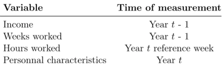
Variable Time of measurement

Income Yeart- 1

Weeks worked Yeart- 1

Hours worked Yeartreference week Personnal characteristics Yeart

Table 1.1: Variables and time of measurement in the Census/NHS of year t

no discrepancy between fiscal and census data for the 95th_{and 99}th_{percentiles of total income} between 1980 and 2005. Data from the 2006 census measure the 99.9th _{percentile of total} income closely, while data from the 2001 census underestimate it slightly. Still, the total rise of the 99.9th _{percentile between 1980 and 2005 is the same in both data sources. Since the} numerator of hourly wages, employment income, is the main component of total income, we contend that employment income is also measured accurately and consistently in census data.

1.2 Hourly compensation in the Canadian census

The Census/NHS does not report hourly compensation directly. However, we can estimate it from other variables. As Table1.1shows, the questions about income and weeks worked refer to the previous year. By contrast, the question about hours refers to hours worked in the week before filling the questionnaire, the so-called reference week. Therefore, we cannot obtain a measure of hourly compensation for respondents who worked only either in yeart or in year t- 1. Similarly, measurement error can happen for workers who are active in both years but change their labour supply over time. Although we do not know the number of hours typically worked by the respondent in the previous year, a question asks if most of the weeks worked were full-time (30 hours or above).

In order to measure hourly compensation as accurately as possible, we thus focus on workers who meet the following criteria :

• Workers must have worked 30 hours or more during the reference week of yeart • Workers must have worked at least 40 weeks in yeart - 1.

• Most of these weeks must have been worked full-time.

We refer to workers who meet these criteria as full-time workers. Note that our sample selection has an asymmetric impact on wage measurement errors. For instance, consider the case of a respondent who usually works 30 hours a week. A respondent who worked 40 hours in the reference week would be included in our sample, and the measurement of his wage would be biased downward. However, if the same respondent worked 20 hours in the reference week 6

(23)

instead, a situation which would have resulted in a measured wage that is biased upward, the observation would be excluded from our sample.

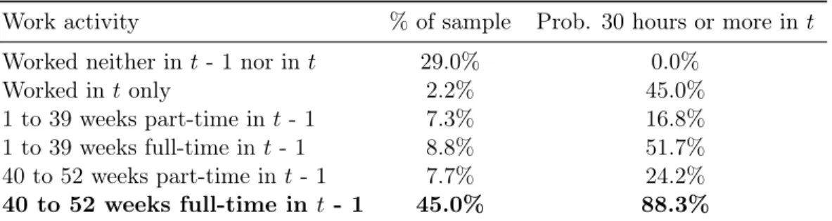
Work activity % of sample Prob. 30 hours or more int Worked neither int - 1 nor int 29.0% 0.0%

Worked intonly 2.2% 45.0%

1 to 39 weeks part-time int- 1 7.3% 16.8% 1 to 39 weeks full-time int - 1 8.8% 51.7% 40 to 52 weeks part-time int - 1 7.7% 24.2%

40 to 52 weeks full-time in t - 1 45.0% 88.3%

Table 1.2: Work activity and conditional probability of working full-time in the reference week, respondents aged 15 and above, 2010-2011 population

Table 1.2shows the distribution of work activity of all respondents aged 15 and above in the NHS. Workers who have worked mostly full-time for 40 weeks or more during year t - 1 are more likely to work full-time during the reference week of year t by a wide margin (88.3%). The sample we use in our study covers 45.0%×88.3%

100%−29.0%−2.2% = 57.8% of the active population in

year t−1. Thus, as long as full-time labor supply does not vary too much between years

t−1andt, our findings are a good reflection of the wage trends faced by Canadians active in the labour market over the last three decades. Part A of the Online appendix has the same information for each of the 7 years included in this study.

Our selection criteria induce truncation bias relative to our target population (full-time workers at a given point in time), most importantly by excluding low earners who move in and out of the labour market. However, the results from Part A of the appendix suggest that the extent of this bias has not varied much through time, since the conditional probability of working full-time in the reference week has been remarkably stable for respondents working more than 48 weeks mostly full-time in the last year, who make up the bulk of our sample.

We use the sum of wages, self-employment income and income from a non-incorporated farm business as our measure of employment income. The question concerning hours worked in the census includes hours worked in one’s own business. Our choice of employment income thus ensures that both the numerator and the denominator of hourly compensation refer to the same concept of work. In our study, we use the terms hourly compensation and hourly wage interchangeably since "wages" include self-employment income. Dollar amounts are in 2010 dollars, unless stated otherwise. We use the national CPI (Statistics Canada,2015) to convert nominal wages in 2010 constant dollars. Hours are censored at 84 (7×12).

(24)

Since some non-incorporated businesses incur losses during the year, respondents might have a negative hourly compensation. This poses a problem when using the logarithm function. Therefore, all of our decompositions based on the log of wages exclude values below 1$ per hour. In part B of the Online appendix, we show that excluding negative wages has little impact on the growth and level of inequality.

We carry out several robustness checks in theOnline appendixto ensure that the inclusion of self-employment income in our measure of compensation does not distort our results. First, we show in part C of theOnline appendixthat the ratio of employment income to total income is fairly stable through time, even when the ratio is broken down by income percentile. In particular, this ratio increases little in the top percentiles. Therefore, the rise in top wages does not appear to be a spurious trend caused, inter alia, by business owners paying themselves wages instead of capital income or through other forms of adaptative accounting.

Second, in part F of the appendix, we recompute the results of Table 2.1, considering only workers whose wages make up between 90% and 110% of total employment income (a per-centage above 100% implies some negative self-employment income). The trends and levels for each column are the same in both the original and the modified tables save for the 10th percentile, which increases after 2000 in the modified table, in line with the findings ofFortin and Lemieux(2015). Since the evolution of inequality is driven by the top of the distribution (as shown by parts B and E of the Online appendix), we believe that the small discrepancy between the two measures for bottom percentiles should pose little problem for our analysis. Also, the modified version of Table2.1is easier to compare to other data sources used in the litterature, such as the Labour Force Survey public files. Part F of the appendix includes descriptive statistics computed from the LFS for 2000, 2005 and 2010. The sample used for the LFS includes only respondents who worked at least 30 hours in the reference week and excludes self-employed workers. The 10th_{, 50}th _{and 90}th _{percentiles show roughly the same} trends, although the absolute levels are higher in census data for the median and the 90th percentile. We attribute these differences to our slightly different concept of compensation, which includes some self-employment income, as well as more restrictive sample selection in census data. Indeed, we restrict our sample to workers who have worked full-time in the reference week and more than 40 weeks mostly full-time in the preceding year. This sample selection cannot be replicated with the LFS, which only has information pertaining to hours worked in the reference week. If workers who move in and out of the labour market earn a lower wage on average, it is almost guaranteed that the moments and percentiles computed from the Census will be higher. The lower level of the 10th _{percentile is likely due to the asymetric} effect of measurement error in the Census, caused by respondents who work abnormally high hours in the reference week compared to their usual work schedule.

(25)

Comparing the 99th _{and 99.9}th _{percentiles is more difficult, because the LFS has a smaller} sample size and wages in the public files are censored. For instance, an employee working 2000 hours in 2010 and with a wage at the 99.9th_{percentile calculated from the LFS would have an} employment income of $ 168,260; by comparison, the 99.9th _{percentile of total income in the} 2009 taxfiler population was $ 705,700 (Table 2,Veall,2012). These two figures are difficult to reconcile since the wages (excluding self-employment income) of individuals in the top 0.1% made up 63.3% of their total income in those years (Table 1, Veall, 2012). Furthermore, the discrepancy is unlikely to be explained by differences in the underlying populations since we would expect full-time workers to be no poorer than taxfilers in general, the population sampled by Veall. Therefore, we believe it is best to restrict the comparison between the Census and the LFS public files to middle wage percentiles.

The take-away message from this subsection is that our measure of compensation shows the same trends as the more restrictive measures typically used in the litterature, except for the lowest percentiles. The two trends we seek to explain and decompose in this paper, the rise of agregate inequality and the evolution of the higher percentiles of the wage distribution, are probably little affected by potential measurement errors at the bottom of the distribution. Furthermore, Census data is the only reliable data that goes back to 1980, a feature that is important for assessing the impact of long-term demographic trends on the wage distribution. Finally, ours may be the only data source readily available to assess the very top of the hourly wage distribution.

(26)

(27)

Chapter 2

Descriptive statistics

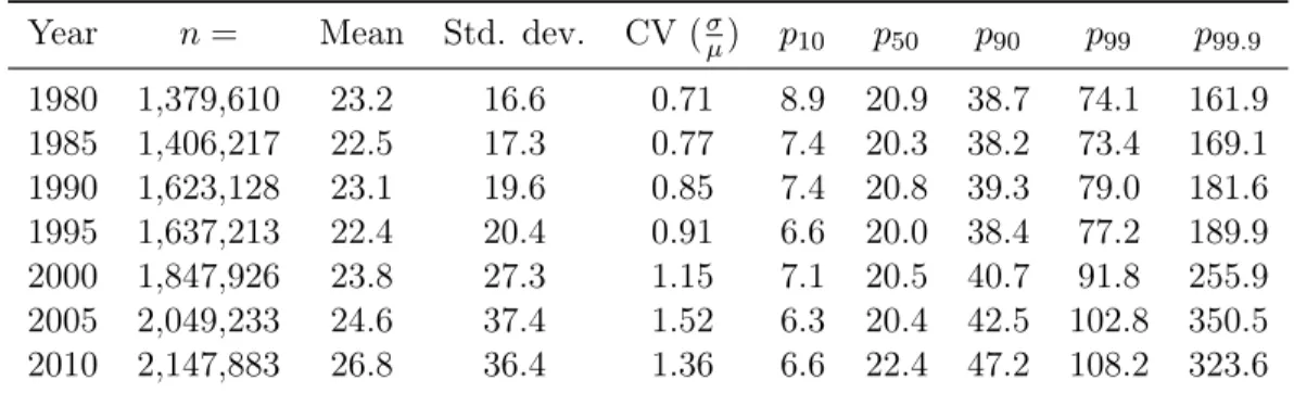
Year n= Mean Std. dev. CV (σ_µ) p10 p50 p90 p99 p99.9

1980 1,379,610 23.2 16.6 0.71 8.9 20.9 38.7 74.1 161.9 1985 1,406,217 22.5 17.3 0.77 7.4 20.3 38.2 73.4 169.1 1990 1,623,128 23.1 19.6 0.85 7.4 20.8 39.3 79.0 181.6 1995 1,637,213 22.4 20.4 0.91 6.6 20.0 38.4 77.2 189.9 2000 1,847,926 23.8 27.3 1.15 7.1 20.5 40.7 91.8 255.9 2005 2,049,233 24.6 37.4 1.52 6.3 20.4 42.5 102.8 350.5 2010 2,147,883 26.8 36.4 1.36 6.6 22.4 47.2 108.2 323.6 Table 2.1: Evolution of the hourly wage distribution among full-time workers (2010 constant dollars)

Table 2.1reports statistics on the evolution of hourly wages among full-time workers between 1980 and 2010. The coefficient of variation (CV) increased sharply starting from 1995. Mean hourly compensation grew by 15.5% between 1980 and 2010, while the median increased by 7.1%. The 10th percentile fell sharply. The90th percentile grew slowly over the period, at a

rate of 0.66% per year. The rapid rise of inequality starting in 1995 coincides with an 85% rise of the 99.9th _{percentile until 2010. For the bottom percentiles, most of the growth has} taken place between 2005 and 2010, a result corroborated by studies based on the Labour Force Survey (Morissette et al.,2013;Fortin and Lemieux,2015).

The 1st percentile is not shown in Table 2.1 since it remains stable at zero. Respondents

who work for a family business without formal arrangements might report zero income but sufficient hours to be included in our sample. We show in sections B and E of the Online appendix that rising inequality in our sample is driven by increasing compensation at the top rather than negative or zero values. In particular, when the observations above the 99.9th

percentile are removed, the growth of the coefficient of variation between 1980 and 2010 falls from 90% to 32%.

(28)

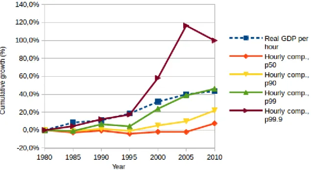
Figure 2.1: Hourly compensation among full-time workers and real GDP per hour, 1980-2005.

In order to put the values of Table2.1into context, Figure2.1compares the evolution of hourly compensation to the evolution of average labour productivity, as measured by real GDP per hour worked (as gathered in U.S. Bureau of Labor Statistics (2012)). The cumulative per-centage growth is normalized to start at 0. Three facts stand out from Figure2.1. Firstly, the

50th,90th and 99th percentiles move roughly in tandem until 1995, when the 99th percentile

begins to grow much more rapidly than the 90th_{. Secondly, the cumulative growth of the}

99th percentile over the period is roughly equal to labour productivity growth : even those

workers located at the 99th percentile have barely kept pace with productivity growth.

Fi-nally, the 99.9th _{percentile grew at the same rate as productivity until 1995, before increasing} dramatically and falling slightly after the Great Recession of 2008.

Note that we ignore sampling variability to simplify the presentation. Given the large size of the sample at our disposal, measurement error and other biases (which are discussed ex-tensively in Chapter 1) are likely to trump sampling variation as the main source of error, even for the highest percentiles. The comparisons with other studies and data sets carried out in Chapter 1 constitute further evidence that the facts we seek to explain are not statistical artifacts, but rather well-documented trends.

The next sub-sections detail the evolution of the hourly wage according to different characteris-tics and quantify the changes that occurred between 1980 and 2010 regarding the composition of the full-time work force.

(29)

2.1 Education

Workers are grouped in five educational categories : no high school (HS) degree, high school degree only, some college (this includes vocational diplomas and CEGEP1_{), bachelor’s degree}

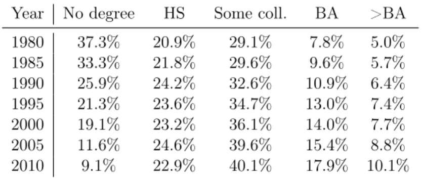
(BA) only and completed graduate degree. Table 2.2 shows that full-time workers are about twice more likely to hold a college degree (BA or higher) in 2010 than in 1980. It also shows that the high school dropout status among full-time workers fell from 37.3% to 9.1% over that period, with a more sudden drop between 2000 and 2005.

Year No degree HS Some coll. BA >BA 1980 37.3% 20.9% 29.1% 7.8% 5.0% 1985 33.3% 21.8% 29.6% 9.6% 5.7% 1990 25.9% 24.2% 32.6% 10.9% 6.4% 1995 21.3% 23.6% 34.7% 13.0% 7.4% 2000 19.1% 23.2% 36.1% 14.0% 7.7% 2005 11.6% 24.6% 39.6% 15.4% 8.8% 2010 9.1% 22.9% 40.1% 17.9% 10.1% Table 2.2: Evolution of educational status among full-time workers

Table 2.3 shows that average hourly compensation fell in 2 educational categories out of 5 between 1980 and 2010, and in 4 categories out of 5 if we use 2005 as the endpoint. Even for BA holders, the group with the fastest wage growth, average hourly compensation increased by only 8.7% over the period, versus 15.5% among all full-time workers. Together, Tables 2.2 and 2.3suggest that rising educational attainments have compensated for sluggish wage growth within skill groups.

Year No degree HS Some coll. BA >BA

1980 19.5 21.2 24.0 32.0 40.7 1985 18.5 20.5 22.6 30.8 39.4 1990 18.3 20.6 23.2 30.8 39.3 1995 17.3 19.7 22.0 28.8 37.0 2000 17.7 20.2 22.9 31.7 39.3 2005 16.7 19.9 23.1 32.9 40.5 2010 17.7 21.0 24.8 34.8 41.6 Total growth, 1980-2005 -14.5% -6.1% -3.8% +2.7% -0.4% Total growth, 1980-2010 -9.3% -0.9% +3.5% +8.7% +2.4%

Table 2.3: Mean hourly compensation among full-time workers, by year and education (2010 constant dollars)

1_{The CEGEP is an institution specific to Quebec. Students can earn either a terminal 3-year diploma that}

(30)

The analysis in this paper assumes that the return to education is strictly causal. Obviously, the magnitude of the rise in education levels in Table 2.2 suggests that other factors might have affected the impact of education on wages. For instance, if workers with a given ability level acquire more education in 2010 than they did in 1980, the slow growth within educational categories in Table2.3 might simply be caused by composition effects. Fortunately, the liter-ature suggests that treating the return to education as causal is a reasonable assumption for a first pass analysis, since the bias caused by omitting ability is typically small (Card,1999). A separate but related issue is that of the quality of education, which might have changed during the last 30 years. Since defining and measuring the quality of education is well beyond the scope of this paper, we assume that the quality of schooling is constant through time.

Year No degree HS Some coll. BA >BA

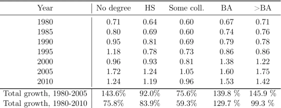
1980 0.71 0.64 0.60 0.67 0.71 1985 0.80 0.69 0.60 0.74 0.76 1990 0.95 0.81 0.69 0.79 0.78 1995 1.18 0.78 0.73 0.86 0.86 2000 0.96 0.93 0.81 1.38 1.22 2005 1.72 1.24 1.05 1.60 1.75 2010 1.24 1.19 0.96 1.53 1.42 Total growth, 1980-2005 143.6% 92.0% 75.6% 139.8 % 145.9 % Total growth, 1980-2010 75.8% 83.9% 59.3% 129.7 % 99.3 % Table 2.4: Coefficient of variation of hourly compensation, by year and education

Table2.4shows the evolution of the coefficient of variation of hourly compensation. Inequality growth was substantial within each group but was highest among college-educated workers. The coefficient of variation does not increase monotonically with education, but has a U-shaped relation, a finding that differs from studies based on US data (Lemieux,2006)2_{. This}

might be caused by higher measurement error among full-time workers with less education, especially if their labour supply varies more over time.

Using either 1980 or 2005 as a reference year for within-group variances, we find that weighting the variances with the composition of 2005 rather than 1980 results in a higher variance in both cases. Repeating this exercise using 1980 and 2010 shows that the composition of 2010 also results in the highest residual inequality. It follows that rising educational attainments should explain part of the increase in residual inequality.

(31)

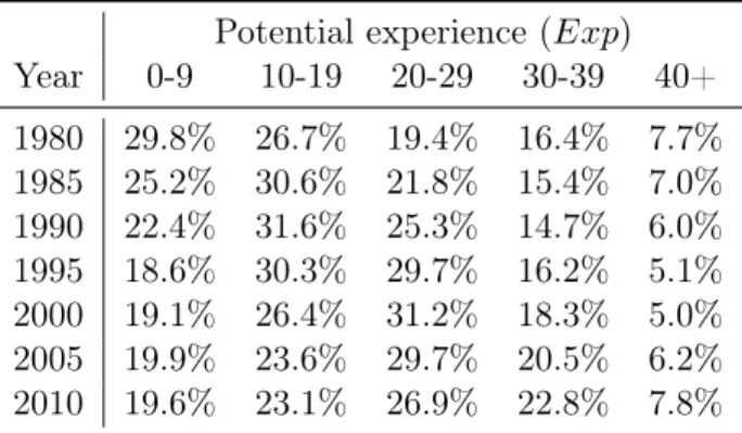
Potential experience (Exp) Year 0-9 10-19 20-29 30-39 40+ 1980 29.8% 26.7% 19.4% 16.4% 7.7% 1985 25.2% 30.6% 21.8% 15.4% 7.0% 1990 22.4% 31.6% 25.3% 14.7% 6.0% 1995 18.6% 30.3% 29.7% 16.2% 5.1% 2000 19.1% 26.4% 31.2% 18.3% 5.0% 2005 19.9% 23.6% 29.7% 20.5% 6.2% 2010 19.6% 23.1% 26.9% 22.8% 7.8%

Table 2.5: Evolution of potential experience among full-time workers

2.2 Potential experience

We define potential experience as Exp = Age −Years of schooling −6. Since the 2006

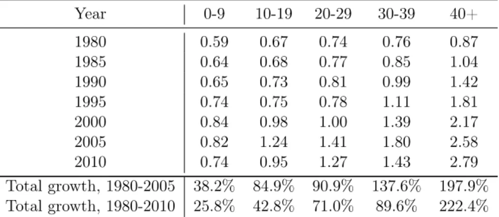
census and the NHS do not measure years of schooling, we allocate them based on the highest degree completed and demographic characteristics. Part D of the Online appendixdetails the procedure. Table2.5 shows the evolution of potential experience in our sample. Almost 27% of full-time workers are part of the category with 20-29 years of experience in 2010, up from 19.4% in 1980. Conversely, the 0-9 category underwent a 10% decline over the same period. Table 2.6shows that average compensation grew in every experience category between 1980 and 2010. Interesingly, hourly compensation growth was fastest in the categories that also experienced the biggest increase in demographic weight. In particular, growth in the 20-29 category was faster than average compensation growth among all full-time workers. The inter-action of this trend with population aging explains a significant proportion of compensation growth between 1980 and 2010. This pattern differs from the trends in Tables 2.2 and 2.3, where rising educational attainments offset stagnating wages within each category. Note that the unconditional wage gap between younger and older workers has expanded over the period. Finally, Table 2.7 shows that within-group inequality increases monotically with experience, in agreement with a model of human capital accumulumation in which workers invest in on-the-job training at differing rates (Mincer, 1974). The relationship between experience and inequality is much more convex in 2005 and 2010 than in 1980. Regardless of the reference year for within-group variances, the aging of the workforce increases residual inequality.

2_Lemieux₍₂₀₀₆_{) uses the log of wages. Calculating the variance of the log with Canadian data yields the}

(32)

Year 0-9 10-19 20-29 30-39 40+ 1980 19.6 25.1 25.7 24.9 20.6 1985 18.2 24.04 25.0 24.2 19.9 1990 18.7 24.0 25.8 24.7 20.1 1995 17.6 22.8 24.8 24.0 19.5 2000 18.6 24.7 25.8 25.3 20.6 2005 18.4 25.5 27.3 26.6 21.7 2010 20.4 27.8 30.0 28.5 23.6 Total growth, 1980-2005 -6.1% 1.5% 6.1% 7.0% 5.4% Total growth, 1980-2010 4.5% 10.7% 16.7% 14.7% 14.6%

Table 2.6: Mean hourly compensation among full-time workers, by year and potential experi-ence (2010 constant dollars)

Year 0-9 10-19 20-29 30-39 40+ 1980 0.59 0.67 0.74 0.76 0.87 1985 0.64 0.68 0.77 0.85 1.04 1990 0.65 0.73 0.81 0.99 1.42 1995 0.74 0.75 0.78 1.11 1.81 2000 0.84 0.98 1.00 1.39 2.17 2005 0.82 1.24 1.41 1.80 2.58 2010 0.74 0.95 1.27 1.43 2.79 Total growth, 1980-2005 38.2% 84.9% 90.9% 137.6% 197.9% Total growth, 1980-2010 25.8% 42.8% 71.0% 89.6% 222.4%

Table 2.7: Coefficient of variation of hourly compensation, by year and potential experience

(33)

2.3 Gender

Year Women Men 1980 31.4% 68.6% 1985 34.2% 65.8% 1990 37.8% 62.2% 1995 38.7% 61.4% 2000 40.2% 59.8% 2005 41.1% 58.9% 2010 42.6% 57.4%

Table 2.8: Evolution of gender among full-time workers

Table 2.8 shows that the proportion of women among full-time workers rose from 31.4% in 1980 to 42.6% in 2010. Since women have lower wages than men, as shown in Table 2.9, their entry in the labour market can increase between-group inequality. Table 2.9also shows that inequality is lower among women and has grown more slowly for them during the period, reducing the growth of residual inequality. Since residual inequality is the biggest component of total inequality, the increased labour force participation of women is likely to have curbed the growth of the variance of wages. Lemieux and Riddell (2015) find that men represented 81.2% of the top 1% in 2005, one explanation for why within-group inequality is much lower among women.

Average CV

Year Women Men Women Men

1980 17.8 25.7 0.55 0.71 1985 17.9 24.9 0.57 0.79 1990 18.9 25.7 0.62 0.89 1995 19.2 24.5 0.64 0.98 2000 20.3 26.1 0.77 1.25 2005 21.2 27.0 0.90 1.70 2010 23.6 29.1 0.81 1.54 Total growth, 1980-2005 19.1% 5.1% 63.6% 139.4% Total growth, 1980-2010 32.6% 13.2% 47.3% 116.9%

Table 2.9: Mean (in 2010 constant dollars) and coefficient of variation of hourly compensation, by year and gender

(34)

2.4 Immigrant status

Average CV

Year Natives Immigrants Natives Immigrants

1980 23.1 23.6 0.71 0.72 1985 22.4 23.0 0.75 0.85 1990 23.1 23.5 0.80 1.02 1995 22.5 22.1 0.86 1.09 2000 23.8 23.6 1.11 1.27 2005 24.9 23.5 1.45 1.77 2010 27.1 25.6 1.34 1.42 Total growth, 1980-2005 7.8% -0.4% 104.2% 145.8% Total growth, 1980-2010 17.3% 8.5% 88.7% 97.2%

Table 2.10: Mean (in 2010 constant dollars) and coefficient of variation of hourly compensation, by year and immigrant status

The share of immigrants in the full-time workforce has risen slightly between 1980 and 2010, from 21.1% to 23.3%. Table 2.10 shows a reversal in the relative position of natives and immigrants : starting in 1995, hourly compensation becomes higher for natives than for im-migrants. This reversal can be explained by other observable characteristics : for instance, native Canadians are aging faster than immigrants and earn higher wages as a result of their higher experience. Boudarbat and Lemieux (2014) also find that immigrants now get lower returns on their education and are increasingly penalized if their language skills are lacking. Table2.10shows that inequality has grown faster among immigrants. This trend is consistent with the sharp decline that occured at the bottom of the wage distribution of immigrants, another fact documented inBoudarbat and Lemieux(2014).

(35)

Chapter 3

Results

3.1 Variance decomposition

The following is true for any pair of random variables :

V ar[Y] =EX[V ar[Y|X]] +V arX[E[Y|X]] (3.1)

If Y in equation (3.1) measures wages and X are observable characteristics, the first term on the right-hand side corresponds to residual inequality and the second term, to between-group inequality. We use this formula to compute the respective contributions of residual and between-group inequality to the evolution of V ar[Y]between two periods :

V ar[Yt]−V ar[Ys] = EXt V ar[Yt|X] −EXs V ar[Ys|X] (3.2) + V arXt E[Yt|X]−V arXs E[Ys|X] .

Xtdenotes the distribution of observable characteristics at timet, andYt|Xthe conditional dis-tribution of wages at timetfor a given vector of characteristics. For instance,EXt

V ar[Ys|X]

(36)

(I) + (II) gives the contribution of residual inequality, while (III) + (IV) represents the con-tribution of between-group inequality. (I) captures changes in residual inequality between s and t that are caused solely by the evolution of within-group variances : the composition of the workforce is held fixed. One important point from Section2 is that wage inequality has increased within every education level, every experience category, and so forth. This pervasive rise in within-group variances is quantified by term (I). By contrast, (II) captures the inter-action of demographic changes and heteroscedasticity. Within-group variances are set to a baseline level, and the composition of the workforce varies over time. For instance, if educated workers’ wages are more dispersed, the impact of increased schooling on residual inequality will be captured by this term. (III) quantifies the impact of changing skill differentials, such as the return to schooling or experience. Finally, (IV) represents the contribution of a change in the dispersion of observable characteristics when skill returns are fixed.

Conceptually, (I) and (III) quantify the impact of changes in the wage structure on resid-ual and between-group ineqresid-uality, respectively. The skill distribution of year t is used as a counterfactual and the wage structure is allowed to vary. Similarly, (II) and (IV) capture the influence of composition effects on residual and between-group inequality. The composition of the workforce varies while the wage structure of yearsserves as a counterfactual.

To compute the decomposition, we drop every observation with hourly compensation below 1$ and use the log of wages in order to remove the effect of a changing mean on the vari-ance. Respondents are allocated to a cell that corresponds to their gender, immigrant status, potential experience and education categories (the categories used are the same as in Section 2). Table3.1 presents the results when the skill distribution of 1981 (t= 1981) and the wage

structure of 2006 (s= 2006) are used.

Total variation = 100%

Residual inequality = 84.5% Between-group inequality = 15.5% Structure (I) Composition (II) Structure (III) Composition (IV)

76.9% 7.7% 12.9% 2.6%

Table 3.1: Variance decomposition, skill distribution of 1981, wage structure of 2006 As foreshadowed by Section 2, (I), the component linked to within-group variances is the dominant factor. Composition effects account for only7.7%/84.5% = 9.1%of the increase in

residual inequality. Since wage inequality is much lower among women in the wage structure of 2006, the entry of women in the labour force over the period offsets the impact of rising educational attainments and experience levels on residual inequality. (III) is quantitatively important because the wages of dropouts and younger workers have fallen substantially be-tween 1981 and 2006. The wage gap bebe-tween natives and immigrants, which was mostly absent in 1981, has expanded substantially over the period, also contributing to the between-group, structural component. Table3.2shows the results with the wage structure of 2011.

(37)

73.6% 11.9% 12.4% 2.2%

Table 3.2: Variance decomposition, skill distribution of 1981, wage structure of 2011 Total variation = 100%

87.1% -2.5% 24.8% -9.4%

Table 3.3: Variance decomposition, skill distribution of 2006, wage structure of 1981 Table3.3shows the same decomposition using the wage structure of 1981 (s= 1981,t= 2006).

The wage structure in 1981 showed much less heteroscedasticity, which explains why composi-tion effects play no role in the rise of residual inequality. Again, the biggest contribucomposi-tion comes from a dramatic rise in within-group variances, and using either 2011 or 2006 as the endpoint does not affect the results. Since more women were part of the labour force in 2006/2011 than in 1981, paying 2006/2011 workers according to the wage structure of 1981, with its larger gender wage gap, results in a higher contribution of (III). Also, educational attainments and potential experience are more dispersed in 2006/2011, which magnifies the impact of expand-ing wage gaps and results in a higher contribution of (III). Finally, (IV) shows that if the wage structure of 1981 would have prevailed, demographic changes such as increased educational attainments among younger cohorts would have lowered between-group inequality.

Residual inequality = 85.5% Between-group inequality = 14.5% Structure(I) Composition (II) Structure (III) Composition (IV)

85.8% -0.3% 26.5% -12.0%

Table 3.4: Variance decomposition, skill distribution of 2011, wage structure of 1981 Although our variance decomposition incorporates the effect of top wages, they are only based on the first two moments of the wage distribution. The next section addresses this limitation by focusing on several counterfactual percentiles.

(38)

3.2 Conterfactual percentiles

Suppose we would like to know the wage distribution that would have prevailed in 2006 if 2006 workers had been paid with the 1981 wage structure. The simplest way to obtain such a distribution is to re-weight the distribution of 1981 characteristics in order to make it identical to the 2006 distribution. Formally, ifX denotes workers’ characteristics, we want to find Ψi such that :

P(X=xi|Y ear= 1981)×Ψi =P(X =xi|Y ear= 2006) (3.3) for each skill group i. When workers are grouped into a number of mutually exclusive cells, the computation ofΨi is trivial :

Ψi =

P(X=xi|Y ear= 2006)

P(X=xi|Y ear= 1981). (3.4)

In order to get more accurate results, we do not group any of the 4 characteristics into categories. Since potential experience becomes a continuous variable for the years in which it is imputed, P(X = xi|Y ear = yyyy) might take zero values for some combinations of characteristics and years. It follows that 3.4 cannot be used directly to compute Ψi. One

way to sidestep this problem is to use probability laws to avoid the direct computation of P(X =xi|Y ear =yyyy). Using the law of total probability and Bayes’ theorem, we obtain

the following formula :

Equation (3.5) is an example of the DFL (DiNardo, Fortin, and Lemieux,1996) method. The terms P(Y ear = yyyy) are sample proportions that are easy to compute, while the terms

P(Y ear = yyyy|X = xi) can be estimated by any discrete choice model. We use a logit

model where the regressors are education, gender, potential experience (linear and squared) and immigrant status.

Using this formula, we compute selected counterfactual percentiles of the wage distribution, using both 1981 and 2011 as reference years for the composition of the workforce. Now, 22

(39)

suppose that the evolution of the distribution of wages between 1981 and 2011 is caused only by composition effects. The graphs of the counterfactual percentiles will form two horizontal lines that will bound the graph of the percentile under consideration, since the composition of the workforce is held constant in counterfactual scenarios. On the contrary, if changes in the distribution are caused solely by changes in the wage structure, the graphs of the counterfactual percentiles are going to be superimposed on the graph of the observed percentile. Thus, a large gap between the counterfactual percentiles and the true percentile indicates that composition effects drive the evolution of wages at this percentile.

Figure3.1shows that average compensation stagnates or falls by one dollar per hour over the period if the four characteristics of Section2are held constant (at their levels of 1981 or 2011). The fall is steeper for the median, as can be seen from Figure3.2. Median compensation drops between 1.7 and 2.8 dollars per hour when we fix the workforce’s composition. Perhaps more surprisingly, the situation is similar for the 90th_{percentile : a 22% percent gain over the period} essentially vanishes when composition effects are removed (Figure3.3).

Figure 3.1: Average hourly compensation among full-time workers, actual and conterfactual with composition of year B (2010 constant dollars)

(40)

Figure 3.2: Median hourly compensation among full-time workers, actual and conterfactual with composition of year B (2010 constant dollars)

Figure 3.3: Hourly compensation among full-time workers, 90th _{percentile, actual and} conter-factual with composition of year B (2010 constant dollars)

(41)

99th _percentile

Education 1980 2005

No degree 53 52

HS degree 56 63

Trade certificate 56 60

CEGEP, non-university diploma 57 69 University certificate < BA 71 88 B.A. 94 140 University certificate > BA 109 151 Medicine 185 250 Master’s degree 98 178 Ph.D. 101 158

Table 3.5: Evolution of the 99th _{percentile of hourly compensation by education group (2005} constant dollars)

Figures 3.4 and 3.5show the evolution of the 99th _{and 99.9}th _{percentiles, respectively.} Inter-estingly, the 99th _{percentile and the 99.9}th _{percentile both grow more slowly in counterfactual} scenarios, especially when the skill distribution is held constant at its 1981 level. Table 3.5 provides the intuition behind this result. If we look at the 99th _{percentile by education group,} we see that the rapid increase of top wages essentially happened among full-time workers with a bachelor’s degree or above. When the skill distribution of 1981 is used, the categories that generate much of the rise in top incomes are under-represented in the data. Since workers in 1981 were half as likely as 2006 workers to hold a college degree, the effect of the resulting difference is quite important. However, when the composition of 2011 is used, the counterfac-tual and accounterfac-tual 99.9th _{percentiles move in tandem, indicating that composition effects begin} to lose their explanatory power at this level in the wage distribution.

In summary, composition effects account for a diminishing but still substantial part of hourly compensation growth as we look towards higher percentiles. In particular, they explain a large proportion of the growth of the 90th _{and the 99}th _{percentile, a fact not visible from the} variance decompositions. Section3.1showed that composition effects explain a relatively small portion of the rise in inequality; this section shows that this is because they do not explain the rise of very high wages. The substantial growth of within-group variances appears indeed to be caused by the growth in compensation among the top wages (mostly the top 0.1%), the change in the rest of the distribution being largely explained by variations in observable characteristics.

(42)

Figure 3.4: Hourly compensation among full-time workers, 99th _{percentile, actual and} conter-factual with composition of year B (2010 constant dollars)

Figure 3.5: Hourly compensation among full-time workers, 99.9th _{percentile, actual and} con-terfactual with composition of year B (2010 constant dollars)

(43)

Conclusion

This paper uses confidential census data and the recent NHS to identify and explain features of the change in wage inequality in Canada between 1980 and 2010. The main findings are as follows.

1. Wages within educational and potential experience groups have stagnated between 1980 and 2010.

2. Hourly compensation growth among full-time workers is driven largely by the aging of the workforce and by rising educational attainments. Once we remove the wage effects of changes in the composition of the labor force (the so-called “composition effects”), average hourly compensation falls by 1% to 8% over the period.

3. The aging of the workforce and the concomitant growth of potential experience has partly offset slow wage growth within skill groups, but this aging effect has arguably run its course.

4. Between 75% and 85% of the increase in wage inequality between 1980 and 2010 is explained by the increase of within-skill-groups inequality, that is, by factors other than composition effects or rising skill differentials.

5. The growth of percentiles up to the 99th _{is mostly driven by changes in the composition} of the workforce.

6. An immediate corollary of (4) and (5) is that the growth of within-group variances, the most important factor in the growth of inequality, must be caused by the growth of percentiles higher than the 99th_{. Section} _3.2_{also shows that composition effects do not} account for the rise of wages in the top 0.1% of the distribution.

7. Section E of the Online appendix shows that the growth of inequality between 1980 and 2010 falls from 90% to 32% when the observations in the top 0.1% are removed, confirming the intuition that these observations drive the growth of inequality.

(44)

More generally, the slow growth of wages within skill groups appears to be caused by deep macroeconomic trends. Karabarbounis and Neiman(2014) find that the labour share of income is decreasing in most countries and industries since 1980, and that half of that decline is caused by a fall in the relative price of investment goods. The fact that the decline of the labour share is a worldwide phenomenon suggests that slow wage growth (relative to output) is not caused by circumstances specific to Canada, and that further research is needed to pin down the exact forces behind the decline of the labour share of income.

Our findings also call into question the effectiveness of policies that seek to address growing inequality or stagnant wages by subsidizing the accumulation of human capital. Most of the rise in wage inequality occured within worker categories, with skill differentials explaining only a small part of the total rise. Likewise, wage growth has lagged behind GDP growth in spite of substantial increases in educational attainments and potential experience. Although subsidizing education might be desirable in its own right, other policies must be enacted if curbing the rise of inequality is a policy objective.

(45)

Online appendix

The online appendix is hosted at the following address : http://www.cedia.ca/sites/cedia.ca/files/onlineappendix_xl.xlsx

Part A contains tables detailing the labour supply of all respondents in the Census, for every year.

Part B compares the evolution of inequality when negatives wages are excluded from our sample to the results obtained from the full sample.

Part C shows the proportion of employment income in total income for each percentile of total income.

Part D shows details on the allocation of years of schooling in the 2006 census and the NHS. Part E compares the evolution of inequality when wages in the top 0.1% are excluded from our sample to the results obtained from the full sample.

(46)

(47)

Bibliography

Boudarbat, Brahim and Thomas Lemieux (2014), “Why are the Relative Wages of Immigrants Declining? A Distributional Approach.” Industrial and Labor Relations Review.

Boudarbat, Brahim, Thomas Lemieux, and W. Craig Riddell (2010), “The Evolution of the Returns to Human Capital in canada, 1980–2005.” Canadian Public Policy, 36, 63–89. Brochu, Pierre, Louis-Philippe Morin, and Jean-Michel Billette (2014), “Opting or Not Opting

to Share Income Tax Information with the Census: Does It Affect Research Findings?” Canadian Public Policy, 40, 67–83.

Card, David (1999), “The Causal Effect of Education on Earnings.” Handbook of labor eco-nomics, 3, 1801–1863.

DiNardo, John, Nicole M. Fortin, and Thomas Lemieux (1996), “Labor Market Institutions and the Distribution of Wages, 1973-1992: A Semiparametric Approach.” Econometrica, 64, 1001–1044.

Fortin, Nicole, David A. Green, Thomas Lemieux, Kevin Milligan, and W. Craig Riddell (2012), “Canadian Inequality: Recent Developments and Policy Options.” Canadian Public Policy, 38, 121–145.

Fortin, Nicole M. and Thomas Lemieux (2015), “Changes in Wage Inequality in Canada: An Interprovincial Perspective.” Canadian Journal of Economics/Revue canadienne d’économique, 48.

Frenette, Marc, David A. Green, and Kevin Milligan (2007), “The Tale of the Tails: Cana-dian Income Inequality in the 1980s and 1990s.” Canadian Journal of Economics/Revue canadienne d’économique, 40, 734–764.

Frenette, Marc, David Alan Green, and WG Picot (2004), Rising income inequality in the 1990s: An exploration of three data sources. Analytical Studies, Statistics Canada.

Green, David and Benjamin Sand (2015), “Has the Canadian Labour Market Polarized ?” Canadian Journal of Economics/Revue canadienne d’économique, 48.

(48)

Green, David A. and Kevin Milligan (2010), “The Importance of the Long Form Census to Canada.” Canadian Public Policy, 36, 383–388.

Karabarbounis, Loukas and Brent Neiman (2014), “The Global Decline of the Labor Share.” The Quarterly Journal of Economics, 61, 103.

Lemieux, Thomas (2006), “Increasing Residual Wage Inequality: Composition Effects, Noisy Data, or Rising Demand for Skill?” American Economic Review, 461–498.

Lemieux, Thomas and W. Craig Riddell (2015), “Top Incomes in Canada: Evidence from the Census.” Technical report, University of British Columbia.

Mincer, Jacob A. (1974),Schooling, Experience and Earnings. Columbia University Press. Morissette, René, Garnett Picot, and Yuqian Lu (2013), “The Evolution of Canadian Wages

over the Last Three Decades.” Technical report, Statistics Canada.

Statistics Canada (2015), “CANSIM Table 326-0021, Consumer Price Index.” URL http: //www5.statcan.gc.ca/cansim/a26?lang=eng&id=3260021.

Statistics Canada, Official Document (2011a), “National Household Survey Income Refer-ence Guide.” Technical Report 99-014-X2011006, Statistics Canada, URL http://www12.

statcan.gc.ca/nhs-enm/2011/ref/guides/99-014-x/99-014-x2011006-eng.pdf.

Statistics Canada, Official Document (2011b), “National Household Survey User Guide.” Tech-nical Report 99-001-X, Statistics Canada, URL http://www12.statcan.gc.ca/nhs-enm/ 2011/ref/nhs-enm_guide/99-001-x2011001-eng.pdf.

U.S. Bureau of Labor Statistics (2012), “Real GDP per Hour Worked in Canada.” URLhttps: //research.stlouisfed.org/fred2/series/CANRGDPH/. Retrieved from FRED.

Veall, Michael R (2010), “2b or Not 2b? What Should Have Happened with the Canadian Long Form Census? What Should Happen Now?” Canadian Public Policy, 36, 395–399. Veall, Michael R. (2012), “Top Income Shares in Canada: Recent Trends and Policy

Implica-tions.” Canadian Journal of Economics/Revue canadienne d’économique, 45, 1247–1272.