Originally published as:

Originally published as:

Passarelli, L., Hainzl, S., Cesca, S., Maccaferri, F., Mucciarelli, M., Rößler, D., Corbi, F., Dahm, T., Rivalta, E. (2015): Aseismic transient driving the swarm-like seismic sequence in the Pollino range, Southern Italy. -

Geophysical Journal International, 201, 3, p. 1553-1567.

Geophysical Journal International

Geophys. J. Int.(2015)201,1553–1567 doi: 10.1093/gji/ggv111

GJI Seismology

Aseismic transient driving the swarm-like seismic sequence

in the Pollino range, Southern Italy

Luigi Passarelli,

Sebastian Hainzl,

Simone Cesca,

Francesco Maccaferri,

Marco Mucciarelli,

Dirk Roessler,

Fabio Corbi,

Torsten Dahm

and Eleonora Rivalta

1_{Section 2.1 “Physics of earthquakes and volcanoes”, GFZ-German Research Centre for Geosciences, Telegrafenberg, D-14473Potsdam, Germany.} E-mail:[email protected]

2_{Institute of Earth and Environmental Sciences, University of Potsdam, Potsdam, Germany}

3_{Seismological Research Centre – National Institute of Oceanography and Experimental Geophysics (OGS), Udine, Italy} 4_{School of Engineering, University of Basilicata, Potenza, Italy}

Accepted 2015 March 3. Received 2015 March 2; in original form 2014 October 24

S U M M A R Y

Tectonic earthquake swarms challenge our understanding of earthquake processes since it is difficult to link observations to the underlying physical mechanisms and to assess the hazard they pose. Transient forcing is thought to initiate and drive the spatio-temporal release of energy during swarms. The nature of the transient forcing may vary across sequences and range from aseismic creeping or transient slip to diffusion of pore pressure pulses to fluid redistribution and migration within the seismogenic crust. Distinguishing between such forcing mechanisms may be critical to reduce epistemic uncertainties in the assessment of hazard due to seismic swarms, because it can provide information on the frequency–magnitude distribution of the earthquakes (often deviating from the assumed Gutenberg–Richter relation) and on the expected source parameters influencing the ground motion (for example the stress drop). Here we study the ongoing Pollino range (Southern Italy) seismic swarm, a long-lasting seismic sequence with more than five thousand events recorded and located since October 2010. The two largest shocks (magnitudeMw=4.2 andMw=5.1) are among the largest earthquakes

ever recorded in an area which represents a seismic gap in the Italian historical earthquake catalogue. We investigate the geometrical, mechanical and statistical characteristics of the largest earthquakes and of the entire swarm. We calculate the focal mechanisms of theMl>3

events in the sequence and the transfer of Coulomb stress on nearby known faults and analyse the statistics of the earthquake catalogue. We find that only 25 per cent of the earthquakes in the sequence can be explained as aftershocks, and the remaining 75 per cent may be attributed to a transient forcing. Theb-values change in time throughout the sequence, with lowb-values correlated with the period of highest rate of activity and with the occurrence of the largest shock. In the light of recent studies on the palaeoseismic and historical activity in the Pollino area, we identify two scenarios consistent with the observations and our analysis: This and past seismic swarms may have been ‘passive’ features, with small fault patches failing on largely locked faults, or may have been accompanied by an ‘active’, largely aseismic, release of a large portion of the accumulated tectonic strain. Those scenarios have very different implications for the seismic hazard of the area.

Key words: Seismicity and tectonics; Statistical seismology; Dynamics: seismotectonics.

I N T R O D U C T I O N

The Pollino range, a mountainous area in Southern Italy (Fig.1), has been affected by an intense seismic swarm that started on the 2010 October 2 and at the time of writing counts more than 6000 events, as

recorded by the Italian seismic network (http://iside.rm.ingv.it, last accessed 2014 October 1). The Pollino range sits on the Calabria– Basilicata regional boundary in an area between the southern Apen-nines and the northern part of the Calabrian arc. The mechanical coupling between those two geological units, the strain field as well

C

15˚48' 16˚00' 16˚12' 16˚24' 39˚48' 40˚00' 0 5

km

Time

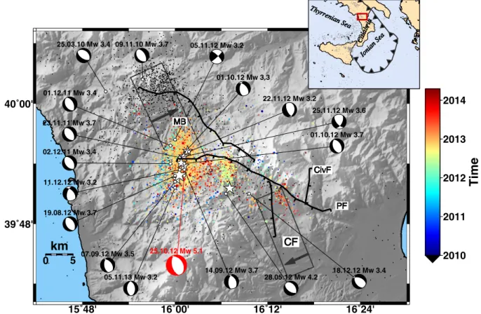
Figure 1.Map of Pollino region and seismicity from 1981 to 2009 (black circles) and colour-coded from 2010. White stars indicate earthquakes with magnitudes larger than 3.5 and focal mechanisms of the largest events are reported. Fault traces are from Frepoliet al.(2011). Rectangles are the surface projections of the faults and arrows indicate the sense of slip according to Basiliet al.(2008) and DISS working group (2010). MB, CF, PF, CivF, stand for Mercure basin Fault, Castrovillari Fault, Pollino Fault and Civita Fault, respectively. In the inset: Map of South Italy with a red box indicating the study area at the border between southern Apennines and Calabrian arc. Lightgrey dots is seismicity (Ml>3) from 1981 to 2010 and the position of Calabrian trench is

reported.

as its tectonic role and the seismic potential of the area are poorly understood so far (Faccennaet al.2011).

The major mapped faults of the region are the Mercure Basin fault in the northern part of the Pollino range, the Pollino fault running WNW–ESE parallel to the mountain chain, the Castrovillari fault which trends NNW–SSE and the approximately N–S trending Civita fault, both branching off the Pollino fault (Cintiet al.1997,2002; Michettiet al.1997; Papanikolaou & Roberts2007; Basiliet al.

2008; Frepoliet al.2011). The Mercure Basin fault in the north and the system of faults in the south are located in two pull-apart basins of the western sector of the Pollino range, the Mercure basin and the Morano-Castrovillari basin, respectively (Martiniet al.2001). In the 1000-yr-long historical catalogue of the Italian earthquakes there are noM>6 events associated with either of those tectonic structures (Rovidaet al.2011). On 1998 September 9, aMw=5.6

normal faulting event ‘reactivated’ seismically the northern part of the Mercure basin (Arrigoet al.2006; Brozzettiet al.2009). The Pollino and Castrovillari faults have been silent, despite the fact that palaeoseismological investigations on both faults suggest at least fourM>6 events occurred within a few thousand years (Cinti et al.1997; Michettiet al.1997). The lack of large earthquakes rank the region as one of the most prominent seismic gaps in the Italian peninsula (Valensise & Guidoboni2000).

Since Fall 2010, some bursts of seismicity together with a high level of background activity have been occurring in the northern part of the Pollino range in an area of about 20×20 km2_{. The individual}

bursts are accompanied by migration of the earthquake hypocentres

and by activation of nearby structures. The largest events recorded during the sequence were aMw = 4.2 on the 2012 May 28 and

aMw =5.1 on the 2012 October 25. At the time of writing, the

latter represents the main shock of the sequence (Masiet al.2014). This seismic sequence activated unknown faults at the margin of the main pull-apart basins of the region.

Several areas of Europe are affected by tectonic earthquake swarms (Apennine chain, Italy, Tj¨ornes Fracture Zone, North Ice-land, Western Alps Italy-France, Corinth Rift, Greece just to men-tion some examples) or swarms of debated origin (Vogtland, Ger-many/Czech Republic), not to mention seismic swarms induced by man-made fluid injections or linked to large water reservoirs (an example close to Pollino is the Pertusillo reservoir in Val d’Agri, see Stabileet al.2014). Seismic swarms are often of mild intensity, but occasionally they do include one or a series of damaging earth-quakes (Keranenet al.2013; McGarr2014). Seismic swarms are poorly understood. Not much is known about the physical mecha-nisms behind their nucleation and development or their potential to influence nearby active fault zones or the short and long-term local seismic hazard.

Systematic analysis of swarm activity has helped identify so far the main differences between seismic swarms and aftershock se-quences (Hainzl & Fischer2002; Hainzl & Ogata2005; Vidale & Shearer2006; Vidaleet al.2006; Lohman & McGuire2007; Hainzl et al.2012): (1) seismic swarms are not dominated by a single large magnitude event occurring at the start of the crisis, rather, seismic swarms may include several earthquakes of similar large magnitude

and the largest events do not occur necessarily early in the se-quences; (2) the temporal evolution of the seismic rate in swarms does not follow the Omori law: the seismic rate may increase and decrease at varying pace and there is no theoretical model yet for the temporal evolution; (3) the frequency-magnitude distribution of shocks in swarms often shows large, still unexplained,b-values and variations inb-values or even deviates significantly from the Gutenberg-Richter (GR) law; (4) seismic swarms generally affect rock volumes much larger than what is suggested by the magnitude of the largest event or events; (5) seismicity in swarms does not light up the entire area directly but shows a significant spread or migration from early on in the sequence. Earthquake-induced static and dynamic stress transfer, thought to be the underlying mecha-nism for aftershock occurrence, cannot explain seismic swarms: an additional forcing is necessary.

It has been proposed that seismic swarms may be linked to a release of tectonic strain intermediate between the instantaneous strain release given by large shocks and slow, silent earthquakes (Peng & Gomberg2010). In many cases, seismic swarms may ac-company slow earthquakes (Lindeet al.1996; Lohman & McGuire

2007; Ozawaet al. 2007). For such cases, the same seismogenic structure shows two different rheological behaviours: aseismic slow slip and regular earthquake, active at the same time in interfingered fault patches. Seismic swarms in subduction megathrust areas seem to repeatedly occur between areas ruptured by larger thrust events and coincide with areas where accumulation of interseismic strain is low (Holtkamp & Brudzinski 2014). Therefore, these regions illuminated by seismic swarms are supposed to mark rheological segmentations of large tectonic structures implying heterogeneity in the stress field not allowing large rupture to propagate. Indeed, strain is released in swarm regions by a combination of seismic brittle failure and aseismic slip (Holtkamp & Brudzinski2014). Furthermore, slow slip events and the associated swarm activity can also trigger large thrust events on adjacent brittle fault segments as in the 2011 Tohoku earthquake (Katoet al.2012).

The physical mechanisms proposed for the origin and evolution of elastic fracturing during ‘natural’ tectonic swarm-like activity include: (i) rupture patches migrating or expanding due to the dif-fusion of pore-pressure lowering the effective normal stress on the rupture plane (Shapiroet al.1997; Hainzl & Ogata2005); (ii) nat-ural hydraulic fracturing inducing elastic failure close to its tips (Dahm et al.2010; Hainzlet al.2012); where a combination of pore-pressure diffusion and hydrofracturing (a hydrofracture leak-ing fluids into pores) is also possible (Hainzlet al.2012) and (iii) slow-slip events or aseismic creep (themselves possibly driven by pressurised fluids) redistributing elastic stress along a large fault area (Lohman & McGuire2007; Peng & Gomberg2010).

All this processes would cause an additional time-dependent forc-ing mechanism actforc-ing on top of the long-term tectonic loadforc-ing and each of them would imply a different level of elastic energy stored in the seismic structures. This may change considerably the hazard of the region. Usually, hazard maps are calculated by assuming a Gutenberg–Richter relation and a maximum magnitude based on the secular tectonic load and historical seismicity of the area. De-creasing the epistemic uncertainties on these assumptions might be critical to obtaining a reliable estimate of short and long-term hazard and the related uncertainties.

Distinguishing between the different physical mechanisms of swarm generation is, in principle, possible if high-quality monitor-ing is available since the mechanisms are linked to different patterns or values in a set of observables. For instance, pore pressure dif-fusion is expected to produce a spreading front of seismicity with

typical velocities of up to several tens of meters per day (Hainzl & Ogata2005). Transient slow slip on faults as the driving force for earthquake swarms is expected to produce measurable deformation at the surface and migration velocity of the accompanying seismic swarm of hundreds of metres per hour (Lohman & McGuire2007). Here we analyse in detail the Pollino sequence from October 2010 to the end of March 2014 using the earthquake locations and wave-form of largest events publicly available athttp://iside.rm.ingv.it. We aim to constrain, among the suggested models for tectonic swarms, the possible driving force and discuss the implications for the seis-mic hazard. We first introduce the area geologically and revise the poor knowledge of historical seismic activity of the Pollino region. We describe in detail the sequence and calculate the focal mech-anisms of the largest events in order to put seismotectonic con-straints on the structures hosting the swarm. We investigate the role of Coulomb stress on the swarm focal area and the silent structure in the Castrovillari basin and the statistics of the events in the swarm and their time evolution. We finally discuss the known structures in the area, how they are affected by transient forcing and how this may inform the hazard assessment for the Pollino region.

Tectonic setting of the Pollino range, Southern Italy

The Pollino range is a complex morpho-tectonic structure located at the northern edge of the Calabrian arc lying at the conjuction between the end of the Southern Apennines and the Calabrian Arc (Ferrantiet al.2009; Faccennaet al.2011, Fig.1). The Pollino range is composed of Meso-Cenozoic shallow water carbonate succession forming a NE-dipping monocline. The present morpho-tectonics, which modified the pre-existing fold-and-thrust belt, may originate from a transpressional regime focused in the lower Pleistocene on a N120o_{E trending fault, often referred as the Pollino shear zone. By}

the middle Pleistocene a counter-clockwise rotation of the carbon-atic block turned the strike-slip regime into a northeast–southwest extension (Schiattarella1998). Such an extensional stress field re-sults in a complex system of normal faults striking nearly parallel to the Apennines chain and bordering the south-western boundary of the Pollino range (Schiattarella1998; Ferrantiet al.2009; Ferranti et al.2014). Other structural investigations using seismic reflection profiles and local network seismicity suggest a still ongoing trans-pressional regime with left-lateral kinematics in the easternmost and offshore part of the Pollino shear zone (Catalanoet al.1993; Ferrantiet al.2009), while inversion of deformation data suggests a transtensional regime of the western part of the range in the Mercure and Morano-Castrovillari basin (Ferrantiet al.2014).

The Pollino region as well as the whole northern Calabria un-dergo uplift at a rate of about 1 mm yr−1 _{(Ferrantiet al.2009).}

Regional geomorphological investigations, constrained by studying the flights of marine terraces at the northern shores of the Ionian, show a long wavelength (∼100 km) uplift of the Pollino region su-perimposed to a smaller scale uplift (∼10 km) (Ferrantiet al.2009; Faccennaet al. 2011). At present, the main northeast-southwest anti-apenninic extensional stress field is the dominant stress field of the central part of the Pollino range. This has been confirmed by geodetic measurements (Serpelloniet al.2005; Ferrantiet al.

2014) and stress tensor inversion of focal mechanisms solutions (Maggiet al.2009; Frepoliet al.2011; Palanoet al.2011; Totaro et al.2013). Therefore, on the local scale the inland ongoing exten-sional stress field within the Pollino range may be accommodated by basin-forming normal faulting (Martiniet al.2001).

The mapped normal faults in the region are the Mercure Basin fault in the northern part of the Pollino chain, the Pollino fault run-ning WNW–ESE parallel to the mountain chain, and two smaller structures branching off the Pollino fault: The Castrovillari fault striking NNW–SSE and the Civita Fault with a NNE–SSW trend (Fig.1) (Maggiet al.2009; Frepoliet al.2011). Recently, Brozzetti et al.(2009) identified a large normal fault structure dipping south-west and bordering the Mercure Basin at the northsouth-west and named Castello Seluci to Piana Perretti and Timpa della Manca Fault. They also proposed this structure as the fault activated by the September 1998Mw 5.6 event. Given, however, the complicated and scarce

surface expression of these faults and the lack of seismic activity associated with them, the rank of the master fault in the southern part of Pollino range is still debated (Michettiet al.1997; Cinti et al.1997,2002; Spinaet al.2009; Palanoet al.2011).

Recent analysis of surface velocities using permanent and a tem-porary Global Navigation Satellite System (GNSS) network shows extension at a rate of 1.5 and 0.5 mm yr−1_{across the Mercure Basin}

fault and the Pollino fault, respectively (Ferrantiet al.2014). There-fore, geodetic data exclude a left-lateral transpressional regime of the inland part of the Pollino shear zone; they show instead nor-mal faulting kinematics with a snor-mall component of dextral motion. However, the large interstation distances, within the GNSS station network result in large uncertainties associated with the measure-ments. When linked to the kinematics of the Southern Apennines, deformation in the southwestern sector of the Pollino range seems to be accommodated primarily by normal faulting with a decrease in extension rate moving from north to south while approaching the end of the Southern Apennines chain (Ferrantiet al.2014).

The crustal properties in the Pollino range are poorly known. Only a few tomographic studies have been carried out so far in the Pollino area (Barberiet al.2004; Orecchioet al.2011; Totaro et al.2014). Barberiet al.(2004) performed a seismic tomographic inversion forvpand thevp/vs ratio using natural earthquakes and

artificial sources in 10 km crustal layers down to 40 km depth. For the Pollino area they found a pronounced anomaly ofvp/vs ratio

with values greater than 1.9 in the Pollino range in the layer 0– 10 km. The anomaly seems to disappear at depths of 10–20 km and it appears again in the 20–30 km layer. A recently published crustal tomographic investigation also using the events of the 2010–2013 swarm sequence found an even larger volume with a prounanced vp/vs anomaly in the shallowest 10 km of the crust (Totaroet al.

2014). This is broadly interpreted by invoking high crack density, presence of fluids or porous rocks filled by fluids (Barberiet al.

2004; Totaroet al.2014). The presence of fluid circulation in terms of deep meteoric water infiltration underneath the Pollino range is also invoked to explain the anomalously low geothermal gradient of the region (Della Vedovaet al.2001).

Historical seismicity

In the 1000-yr-long historical catalogue of the Italian earthquakes (Rovidaet al.2011) there are noM> 6 events associated with either of the faults of the study area. This was first recognized by Omori at the beginning of the last century (Omori1909) and further detailed through historical investigation by referring to this lack of large events as the ‘Pollino seismic gap’ (Valensise & Guidoboni

2000). However, on the 1998 September 9, aMw = 5.6 normal

fault event ‘reactivated’ the Mercure Basin fault (Michettiet al.

2000; Arrigoet al.2006; Maggiet al.2009) having a geometry compatible with the geologically mapped fault (Basiliet al.2008).

On the contrary, the Pollino and Castrovillari faults are still silent although palaeoseismological investigations on both faults suggest severalM>6 events occurred within the last 10 000 yr (Cintiet al.

1997,2002; Michettiet al.1997).

Five historical earthquakes (1693, 1708, 1792, 1825 and 1894) with magnitude comparable or slightly smaller than the 2012 Octo-ber 25 main shock are listed in the parametric catalogue of Italian earthquakes (Rovidaet al.2011). Their inferred epicentral locations are in the northern part of the Pollino range with macroseismic mag-nitudes ranging from 4.5 to 5.5. The earliest event occurred on 1693 January 8 near the supposed intersection of the Pollino and Castro-villari faults (Guidoboniet al.2007; Rovidaet al.2011; Tertulliani & Cucci2014). The 1693 earthquake had an estimated magnitude of 5.7 (Guidoboniet al.2007) which recently has been revised to 5.2 by integrating different historical sources (Tertulliani & Cucci

2014). According to the authors, this earthquake occurred during a year-long sequence of seismic activity felt by the local population suggesting a large similarity with the ongoing seismic sequence. Also the 1708 event was part of a longer sequence that lasted for several months, with the strongest shocks occurring in a three day long period (Camassiet al.2011). This may be an indication that repeating swarm-like sequences characterize the seismicity of the Pollino region.

Chronology of the seismicity

The current activity started at the end of 2010. More than 6000 events (at the time of writing) have been located by INGV, most with shallow (<15 km) hypocentral depth (Govoniet al. 2013; Totaro et al.2013). As documented by Govoniet al.(2013), the seismicity on the Mercure Basin fault seems not to be confined to the fault activated by the 1998Mw=5.6 event (Arrigoet al.2006; Govoni

et al. 2013), but to depict a more complicated system of faults (Govoniet al.2013; Totaroet al.2013). The activity peaked on 2012 October 25 with aMl = 5.2 event striking in the southern

part of the Mercure Basin fault (Govoniet al.2013). The event caused damage in villages around the epicentral area leaving more than hundred families homeless. After about one month, the seismic activity decreased drastically to approximately ten events per day until the beginning of Spring 2014.

In this study, we make use of the locations of earthquakes between 2006 April 16 and 2014 March 27 provided by INGV (downloaded at http://iside.rm.ingv.it). We use the seismicity in the volume given by [15.9E, 16.3E], [39.8N, 40N] and 0–15 km depth (Fig.1). The events in the selected volume are 5728. Of those, 201 events are in the period 2006–September 2010 and the rest belongs to the swarm sequence, while only 124 events have a deeper hypocentral location in the same time window.

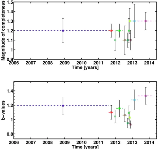
We first check the temporal homogeneity of the catalogue by analysing the temporal evolution of its completeness. We group the events in subsets of 500 and infer the parameters of the frequency-magnitude distribution by using theb-stability method (Woessner & Wiemer2005). The results for the coupled inference ofb-values and magnitudes of completeness (Mc) show the latter being rather

stable in time, taking values between 1.1 and 1.3, while the associ-atedb-values have small variations during the period of high seismic activity (Fig.2). The inferredb-values and magnitudes of complete-ness are also consistent with those inferred using all events in the catalogue. We postpone a detailed analysis of b-values variation until later in the paper after a detailed description of the different phases of the sequence.

2006 2007 2008 2009 2010 2011 2012 2013 2014 0.8 1 1.2 1.4 Time [years] b−values 2006 2007 2008 2009 2010 2011 2012 2013 2014 0.9 1 1.1 1.2 1.3 1.4 1.5 Time [years] Magnitude of completeness

Figure 2. Completeness over time of the seismicity catalogue from 2006 to 2014. In the top and bottom panels are reported the values forMcandb-value

respectively each pair with same colour-code and inferred by grouping 500 events at a time. The horizontal dashed line indicates the non-overlapping time intervals relative to each group and markers are placed at the half of interval. Errors are one bootstrap standard deviation.

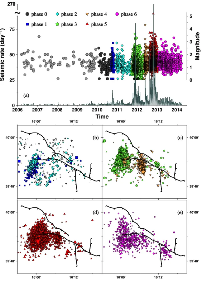
We identify six different phases (1–6) according to major changes in the temporal evolution of the daily rate of activity (Fig. 3). Phase 0 refers to the seismicity that occurred in 2010 before the onset of the swarm. The location errors of the catalogue are on the order of kilometres thus making difficult an accurate analy-sis of the spatial distribution of events. This partitioning can be later refined when precise earthquake locations will be available in order to account also for the spatial separation of the bursts of activity.

The seismicity recorded from April 2006 till the end of 2009 shows a moderate activity (Fig. 3). Almost all activity consisted of microseismicity (Ml ≤3.4). Only one shallow (depth<2 km)

Ml=3.4 event occurred at the end of January 2007 with epicentre

between the easternmost tip of the Mercure Basin fault and the Pollino fault (Fig.1). Although the daily rate of seismicity shows a slow increase from late 2009 until the beginning of 2010, the location of events does not show any sign of spatial clustering. There was an increase in events detected between early 2010 and October 2010 (phase 0). They were also widely spread along the fault traces depicted in Fig.3.

The activity suddenly started to ramp up on 2010 October 2 with a high seismicity rate lasting for less than one month (phase 1). The epicentral locations show NNE alignment with a clear spatial clustering (Fig.3). This sudden increase is followed by almost one year of moderate activity (phase 2) with a few events per day. The epicentres show the same alignment as the previous burst but slightly shifted to the west and to the east (Fig.3). During this phase few tens of events occurred, with scattered epicentres. In September 2011 the

seismic activity showed a fast acceleration (phase 3) until the end of the year followed by a slower deceleration until May 2012. The magnitudes of the events increased and fourM> 3 earthquakes occurred. Their epicentral locations cluster at the northern tip of the previous activity, lighting up a larger area compared with the previous phases 1 and 2 (Fig.3).

At the end of May 2012 the activity migrated eastward and a smaller cluster of events accompanied a shallowMl = 4.3

earth-quake on 2012 May 28 (phase 4 in Fig.3). The event represents the second largest shock of the entire sequence. The rate of activity after theMl=4.3 event showed an Omori-type decay which lasted for

about one month. During this period the seismicity rate decreased to a few events per day. The spatial distribution of these events is nearly N–S, with the largest event located at the southern tip of this small cloud. Events of this phase are tightly confined in space and seem spatially separated from the previously activated area (Figs1

and3).

In June and July of 2012, the seismic rate was less than ten events per day. At the beginning of August (phase 5 in Fig.3) the seismic-ity showed a climax with a faster acceleration of the seismic rate compared with the 2011–2012 bursts of activity. Differently from the previous phases, here the rate of events per day showed isolated peaks together with a long-term gradual increase. These isolated peaks could be related to the presence of aftershocks triggered by the largest events (Ml>3). This seismicity phase occurred over two

months and culminated on 2012 October 25 with aMl=5.2 in the

same epicentral area activated by the onset of the seismicity. During this phase more than tenM>3 events occurred, almost all in the

0

1

2

3

4

5

Magnitude

0

25

50

75

100

Seismic rate (day

−1

)

2006

2007

2008

2009

2010

2011

2012

2013

2014

Time

phase 0

phase 0

phase 1

phase 1

phase 2

phase 2

phase 3

phase 3

phase 4

phase 4

phase 5

phase 5

phase 6

phase 6

~

270

270

(a)

(a)

(b)

(b)

(c)

(c)

(d)

(d)

(e)

(e)

Figure 3.Plot of the different phases of the swarm sequence. (a) Histogram of the daily rate of events from 2006, superposed white bars are events with magnitude above 1.3. Filled symbols is magnitude versus time plot. Different colours and markers refer to phases in which we divided the swarm. (b)–(d) Map of epicentral locations of earthquakes of distinct phases. Large stars in panel (c) and (d) are theMl=4.2 andMl=5.2. Fault traces are reported as in Fig.1

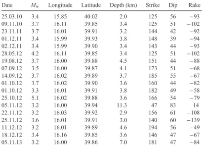
Table 1.Parameters of focal mechanisms.

Date Mw Longitude Latitude Depth (km) Strike Dip Rake

25.03.10 3.4 15.85 40.02 2.0 125 56 −93 09.11.10 3.7 16.11 39.85 3.4 125 51 −102 23.11.11 3.7 16.01 39.91 3.2 144 42 −92 01.12.11 3.4 15.99 39.93 3.8 148 39 −94 02.12.11 3.4 15.99 39.90 3.4 143 44 −93 28.05.12 4.2 16.11 39.85 3.4 125 51 −102 19.08.12 3.7 16.00 39.88 4.5 151 44 −88 07.09.12 3.5 16.00 39.87 4.1 173 51 −68 14.09.12 3.7 16.02 39.89 3.7 185 55 −67 01.10.12 3.7 16.02 39.90 3.6 160 44 −82 01.10.12 3.3 16.01 39.91 3.8 182 49 −58 25.10.12 5.1 16.02 39.88 3.6 166 54 −79 05.11.12 3.2 16.00 39.94 11.3 47 83 14 22.11.12 3.2 16.03 39.92 2.9 156 61 −108 25.11.12 3.6 16.01 39.91 3.0 140 60 −139 11.12.12 3.2 16.01 39.89 4.6 194 56 −49 18.12.12 3.4 16.16 39.85 3.6 146 47 −67 05.11.13 3.2 16.00 39.86 7.0 181 47 −84

area struck by the main shock except for one that occurred further east in the Castrovillari basin.

One month after theMl =5.2 earthquake, on 2012 November

25, the seismicity suddenly dropped to 10 events per day denoting a new phase of activity (phase 6 in Fig.3). Most earthquakes were clustered in and around the area where the main shock occurred, with a significant enlargement of the area affected by the seismicity. During 2013 the activity moved eastwards showing a small cluster right at the intersection of the Pollino and Castrovillari faults. At the time of writing, the sequence is still ongoing, with occasional events above magnitude 3.

Focal mechanisms and Coulomb stress transfer

We calculate the focal mechanisms for theMl >3.2 events in the

catalogue using data from the Italian permanent seismic network. We use the moment tensor inversion method presented in Cesca et al.(2010,2013b), which is based on the fit of full waveforms and amplitude spectra. We obtain 18 double couple solutions for which availability and quality of data allowed us a robust inversion. We find mainly NW-striking normal faulting with centroid depths between 2 and 7 km. A few events have NW-striking oblique mechanisms and centroid depths in the range of 3–5 km. We find one NW-striking pure strike-slip solution with the deepest centroid depth of 11 km (Fig.1). Overall, our results are similar to findings by Totaroet al. (2013). From the distribution of the focal mechanisms we can gain insights into the seismo-tectonic setting of the area, although a more precise relocation of the events is needed in order to image the precise geometry of the structures hosting this seismic sequence. Normal faulting mechanisms occurring in the western seismic cloud show a high degree of similarity across all the magnitudes and a NNW–SSE strike, with the steepest plane dipping southwest (Fig.1). The southwest dipping focal plane is in agreement with the southwestward trending of the depth distribution of hypocentres de-rived from precise relocation of the events within the sequence (Am-atoet al.2012; Govoniet al.2013; Totaroet al.2013). These results seem to show a disagreement between the structure(s) activated by the swarm and the geologically mapped east-dipping Mercure Basin fault (Basiliet al.2008). Moreover, they are also in contrast with the September 1998Mw=5.6 normal faulting with northeastward

dipping plane occurred in the northern sector of the Mercure basin (Arrigoet al.2006), although the conjugate southwestern dipping plane has been proposed by other authors (Brozzettiet al.2009). It is likely that the swarm has been hosted by a different, and so far, unknown blind fault pointing at a more complex tectonic setting of the Mercure basin than a simple graben-like structure.

Moving eastward from the main shock, the two shallow fo-cal mechanisms (FM parameters are reported in Table1) - with hypocentral depths of 3.4 and 3.6 km for the Mw = 4.2 and

Mw = 3.4 events, respectively—show counter-clockwise rotated

strikes (about 25 degrees) and almost parallel to the Pollino ridge and fault trace (Fig.1). The east–west elongation of the swarm, as depicted by the inferred focal mechanisms, may give some hints on the tectonic structure illuminated by the activity, as we describe in the next paragraph, although the uncertainties associated with the inversion procedure deserve caution for a definitive seismotectonic assessment.

If the two separate main clouds of seismicity (Fig.1) are ruptur-ing different segments of the same fault, then this structure could be consistent with the geologically mapped Pollino fault (see Fig.1and Papanikolaou & Roberts2007; Ferrantiet al.2014), being activated now at its westernmost tip. The migration of seismicity farther east late in the sequence (Figs1and3), the events recorded in the past (Frepoliet al.2011) and the location of the largest events during the past four centuries (Rovidaet al.2011) would support the hy-pothesis that a mechanical discontinuity exists running parallel to the Pollino ridge, characterized by low seismic activity. However, with the present few focal mechanisms and without a precise relo-cation of the events, we cannot rule out that a system of sub-parallel normal faults has been activated by the evolution of the sequence.

The presence of a strike-slip mechanism together with the oblique faulting of some events suggests complexity of the stress field, compatible with a transtensional stress field of the region. Ferranti et al.(2014) calculated the slip rate accumulated onto a southwest-dipping normal fault located in the Mercure basin based on GNSS data of surface deformation. They found geodetic slip rate com-patible with normal faulting with a minor right-lateral component of the slip. Independent inversion of focal mechanisms performed on different data collected during the ongoing sequence confirm the presence of few pure strike-slip mechanisms or oblique events (Totaroet al.2013). All this indicates a transtensional setting of the

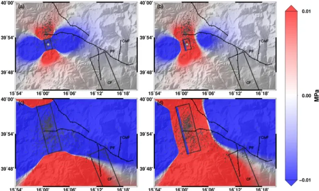
Figure 4.(a) Coulomb stress maps sliced at 3.6 km, and produced by a fault modelling theMw=5.1 largest shock on a receiver fault simulating the Castrovillari

fault (parameter from DISS here). (b) Same as in panel (a) but sliced at 6 km depth. Grey circles in panels (a) and (b) is the seismicity occurred in one month time window after the occurrence of theMw5.1 earthquake on 2012 October 25. (c) Same as previous panel but now causative fault has the longitudinal swarm

extension and size and slip is constrained to produce aMw=6.3 event, Coulomb map refers to 5 km depth. (d) same as in panel (c) but at 10 km depth. Grey

circles in panels (c) and (d) is the seismicity occurred from theMw5.1 earthquake on 2012 October 25 till 2014 of March 27. Seismicity is used to highlight

the extension of the area interested by the swarm activity. Fault traces, names and rectangle of the CF are the same as in Fig.1. The causative fault in the panels are surface projections of the dislocation patch used to calculate the Coulomb stress changes as discussed in the text.

western sector of the Pollino range with a possible rotation of the stress field into pure strike-slip regime at larger depth. Alternatively, the strike-slip component of the oblique faulting can be explained by re-activation of non-optimally oriented structures embedded in a homogeneous extensional stress regime.

Spinaet al.(2009) calculated the static stress transfer in terms of Coulomb stresses assuming the Pollino fault and Castrovillari fault to be in turn causative and receiver faults for an event of about M= 6. They conclude that aM =6 event on the Pollino fault would inhibit slip on the Castrovillari fault (named Frascineto fault in their study), but an event of the same size on the Castrovillari fault may significantly increase the Coulomb stress on the north-western branch of the Pollino fault. They also argue for a primary role of the Castrovillari fault in accommodating extensive tecton-ics, indicating the Pollino fault as a weak mechanical discontinuity capable of being loaded by the Castrovillari fault (Spinaet al.2009). Based on the focal mechanisms of the ongoing sequence, we investigate the role of the static stress transferred by the largest event (Mw=5.1, on 2012 October 25) on the eastern side of the Pollino

range using the Castrovillari fault as a target fault. This analysis complements the one performed by Spinaet al.(2009) because it addresses a possible activation of the Castrovillari fault in terms of static stress interaction. We use only the Castrovillari fault as receiver fault because fault parameters (dip=60o_{, strike=158}o

and rake= −90o_{) are accessible athttp://diss.rm.ingv.it/diss/(Basili}

et al.2008, last accessed 2014 October 1), on the contrary the same information is not available for the Pollino fault. We use the relation by Wells and Coppersmith (1994) to constrain the rupture surface given the moment magnitude of the event, obtaining a rupture area of about 20 km2_{. We model the causative fault as a square dislocation}

(Okada1992) of side 4.5 km, centred at 3.6 km depth (Fig.4). The fault strike (166o_{), dip (54}o_{) and rake (–79}o_{) were set according}

to the focal mechanism solution in Fig.1and the slip (10 cm) was estimated from:M0=G∗A∗s, whereM0is the static seismic moment

calculated in the focal mechanism inversion (Cescaet al.2010),G is the rigidity of the crust (set to 25 GPa), Ais the rupture area andsis the slip. We calculate the Coulomb stress change (CFS) according to the formula:

C F S=τ+μ(σ+p), (1)

whereτis the traction positive in the slip direction on the receiver fault plane,σ is the normal stress on the same plane positive for extension, andμ=0.7 is the friction coefficient. The pore pressure changepis related to the normal stress change according top= Bσ, whereBis the Skempton coefficient, we assume equal to 0.5. As expected, the static stress change induced in the surroundings by the event is very low on the Castrovillari fault, below 0.01 MPa (see Fig.4, panels a and b).

Since the estimated Castrovillari fault parameters are very sim-ilar to the main fault parameters, the Coulomb stress pattern plot-ted in Fig. 4 is practically indistinguishable from the Coulomb stress change acting on faults oriented in the same direction as the main fault. Therefore the pattern from panels (a) and (b) in Fig.4can also be used to consider the stress change induced by the Mw5.1 event on the swarm area, where the focal mechanisms are

all alike.

Given the relatively small extension of the main fault and the uncertainties in the epicentral locations, it is difficult to compare the swarm seismicity following the main event with the computed Coulomb stress change map (Fig.4, panels a and b). Moreover, the

10−4 10−3 10−2 10−1 100 P(M>M *) 0 1 2 3 4 5 Magnitude

(a)

(c)

(b)

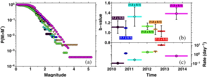
Figure 5.Frequency–magnitude plots in panel (a) and the relativeb-values (panel b) calculated for each phase of the seismic sequence; texts report theMcs

jointly inverted with theb-values. Seismicity rate calculated for each phase is plotted in panel (c). Colours and symbols are the same as in Fig.3. Errors for theb-values andMcs is one bootstrap standard deviation. Horizontal lines in panels (b) and (c) indicate the time period in which the quantities are calculated,

markers are placed in the middle point of the time window.

pattern of the induced Coulomb stress change is strongly depth-dependent, and the low precision in the hypocentral depths does not allow us to appreciate different patterns for the swarm seis-micity at different depths. Nevertheless, it is interesting to notice that the seismicity occurring within one month after the Mw 5.1

event extended mostly northward, coinciding with the positive lobe (enhancing of seismicity) of the Coulomb stress change mapped at shallower depth (Fig.4panel a) and farther beyond it. Although somewhat correlated, the epicentral area of the events that occurred in one month following theMw 5.1 event cannot be entirely

ex-plained by the spatial extent and the intensity of the Coulomb stress increase (see Fig.4panels a and b). In the present case most of the events fall in an area with positive but very low Coulomb stress change (CFS<0.01 MPa; Fig.4), and we argue for an external forcing in play or for a larger strain release rather than only redistri-bution of static stress due to aMw5.1 event. We will return to this

point later in the discussion section, after a more detailed analysis on the swarm evolution.

Additionally, we compute the Coulomb stress change that would affect the area due to a hypothetical rupture as large as the whole area lit up by the swarm activity (see Fig.4panels c and d). We consider a fracture surface of 20 × 10 km, producing a slip of 60 cm (equivalent to aMw=6.3 event using Wells & Coppersmith

(1994) relationship; Fig.4, panels c and d). Such a scenario would account for a hypothetical, very large aseismic slip, that may have affected the swarm area since the beginning of the swarm sequence. Yet, such an exercise represents an overestimation of the total seis-mic moment released by the swarm activity. We find that even in this case the calculated static stresses have low intensity on the Castrovillari fault.

As quantitatively discussed in Passarelliet al.(2013a) and Cesca et al. (2013a), positive variation of the Coulomb stress, even of a small intensity similar to what we find on northern portion of the Castrovillari fault (Fig.4), leads to an increase of triggering probability. The magnitude of the increase of probability scales with the intensity of the Coulomb stress and decreases in time according to the decay rate of aftershocks (Dieterich1994; Passarelli et al.2013). However, the possibility that a major tectonic event is triggered is mainly controlled by the tectonically pre-loaded stresses (Cescaet al.2013a; Passarelliet al.2013), so that the possibility that an earthquake on the Castrovillari fault is triggered due static

stress interaction with seismic events in the Mercure basin cannot be excluded.

Seismic swarm statistics and transient forcing

The relative abundance of small to large magnitude events is de-scribed by the b-value of the frequency–magnitude distribution (Gutenberg & Richter1944). Relative changes ofb-values in space and time are often interpreted as a change in the confining stress within the seismogenic crust. Lowerb-values, indicative of a large proportion of larger size events, correspond to higher confining stress (Schorlemmeret al. 2005). The relative variations of the b-values across a sequence are helpful in identifying changes in the earthquake generation process (Wiemer & Wyss2002). In this sense a careful analysis of the temporal evolution of the frequency-size statistics for each single phase of the sequence may help to constrain the underlying physical processes.

For the Pollino sequence we study the frequency-magnitude dis-tribution of events by using theb-stability method (Woessner & Wiemer2005). The magnitude of completenessMcvaries between

1.1 earlier in the sequence and 1.3 at the end of it (Fig.5a). The b-values oscillate somewhat showing a general feature: Theb-values are larger during periods of lower rate of activity and lower when activity is intense (see Figs5b and c). Also, a general decrease of b-value is observed in the time prior to the main shock.Mcseems

correlated withb-values, so in order to check for a possible inter-dependency, we performed the same analysis after fixingMcto its

highest value of 1.3 finding the same trend.

The observation of decreasingb-values correlated with an in-creasing rate of seismicity seems to be a common characteristic of some tectonic swarms (Hainzl & Fischer2002; Hiemeret al.2012) although the physical mechanisms behind this is still unclear. In volcanic swarms induced by fluids,b-values are considerably large when compared with tectonic seismicity (Wiemer & Wyss2002). Observation of temporal variation of theb-value for the seismic swarm sequence preceding the Augustin 2006 eruption shows the opposite trend we observe for the Pollino swarm (Jacobs & McNutt

2010). There,b-values show an increasing trend over time as the seismicity rate increases at least up to a month before the eruption (Jacobs & McNutt2010). Therefore, the increase in the average size

10

10

10

10

10

10

10

10

Probability density (min

−1

)

10

10

10

10

10

10

10

Interevent time (min)

CVall = 4.1 (2371) CVall = 4.1 (2371) CV0 = 1.2 (24) CV0 = 1.2 (24) CV1 = 1.3 (54) CV1 = 1.3 (54) CV2 = 2.2 (58) CV2 = 2.2 (58) CV3 = 1.9 (340) CV3 = 1.9 (340) CV4 = 1.6 (161) CV4 = 1.6 (161) CV5 = 1.8 (1390) CV5 = 1.8 (1390) CV6 = 1.4 (338) CV6 = 1.4 (338) 10−6 10−5 10−4 10−3 10−2 10−1 100 Probability density 10−1 ₁₀0 ₁₀1 ₁₀2 IET/<IET>

Figure 6.Probability density for interevent times (IETs) of each phase of the sequence. Colours and symbols are for the phases 0–6 in Fig.3. Dot-dashed line are IETs for all data. Coefficient of variation CV are reported together with the number of data above the catalogue completeness. Fine dotted line is exponential distribution with mean equal to six minute, while solid dashed line is power law function∼t−1.5. In the inset same as the main plot but IETs of each sequence are normalized by their mean values.

of events (i.e. mirrored in theb-values in Fig.5) when the seismicity rate is high might suggest another process in play rather than simply fluid-induced seismicity for the Pollino swarm.

We also study the distribution of interevent times by selecting eventsM>Mc=1.3. If the earthquakes in a catalogue can be

mod-elled as a Poisson process, the interevent times follow an exponen-tial distribution (Kagan & Jackson1991). In general, a Poissonian model fits seismicity well only when main shocks are considered, while aftershocks or swarm-like sequences introduce clustering in the earthquake sequences. By means of the coefficient of variation (CV), that is the ratio between the standard deviation and mean of the population of interevent times, we check when interevent times depart from an exponential distribution. Exponential distributed variables have CV=1 while overdispersed data take CV>1 indi-cating a degree of clustering in time usually described well with a power-law behaviour. Swarm-like sequences are expected to have a high degree of clustering (CV>1) and interevent times show self-similarity in a time scale from minutes to days (Hainzl & Fischer

2002; Hiemeret al.2012; Hainzlet al.2012).

As expected, we find a high degree of clustering when we use all data in the sequence (Fig. 6). In detail, CV is close to one before the onset of the swarm (i.e. phase 0) indicating random oc-currence of events, mainly due to the fact that in this time lapse seismicity is small in magnitude (M∼0.5–2.5) and the restriction

to events withM≥Mc=1.3 practically declusters the catalogue.

For all the other phases, CV takes values larger than 1, with em-pirical distribution of interevent time compatible with a power-law model (see Fig.6); only for phase 0 we cannot reject at 5 per cent confidence level the null hypothesis of exponentially distributed in-terevent times. This is similar to fractal temporal clustering found for example for the 2000 and 2008 Vogtland swarms (Hainzl & Fischer2002; Hainzlet al.2012; Hiemeret al.2012). There, a sim-ilar degree of dispersion of interevent times has been interpreted as a common triggering mechanisms across all sequences (Hainzl & Fischer2002). This explanation may apply also to the Pollino sequence.

Earthquakes swarms are usually the result of the interplay be-tween aseismic forcing acting on tectonically loaded structures and earthquake–earthquake self-interaction. In this way, the observed seismicity results from the contribution of two processes: One is re-lated to stress changes rere-lated to aseismic processes, the other one is related to earthquake-induced stress changes. While the second one is interesting for studying earthquake interactions, the first process is of major interest for exploring the initiation mechanism of the whole sequence. A recently published model based on the Epidemic Type Aftershock Sequences (ETAS) model is suitable to separate the two aforementioned contributions buried in the seismicity rate (Hainzl & Ogata2005; Marsanet al.2013).

Table 2.Parameters of ETAS model as discussed in the text.

Region Ntotal Smoothing Nbackground K C(d) α p AIC

Pollino 600 ∞ 22 0.054 0.21 1.68 1.36 356.2

Pollino 600 8 449 0.003 0.0007 2.32 1.06 335.8

The formulation of the temporal ETAS model postulates that seismicity rateλ(t) is given by the sum of a constant background rate μand a time dependent term for earthquake-earthquake triggering given by a combination of earthquake production and Omori law (Ogata1988). Hainzl & Ogata (2005) proposed a modification of the model where the background term μ(t) can account for time variation due to changes in the external aseismic forcing:

λ(t)=μ(t)+

k:tk<t

K eα(M−Mcut)_(c+t−t

k)−p, (2)

where parameterscandpare related to the Omori law,Kandαare related to the empirical magnitude-dependent aftershock productiv-ity. We use in this study an improved method proposed by Marsan et al.(2013) which allows us to systematically separate the relative contribution of transient forcing and earthquake–earthquake trig-gering mechanisms (see also Hainzlet al.2013). The methodology uses an iterative optimization procedure that simultaneously makes inference on μ(t) and the aftershock parameters (second term of eq. 2) by means of the ETAS model. The background rateμ(t) is smoothed by calculating the probability of events being background in a chosen window ofnevents, and then it is used for optimizing the aftershock parameters in eq. (2) via maximum likelihood estima-tion. The algorithm is iterated until all parameters in the right-hand of eq. (2) converge (Hainzlet al.2013; Marsanet al.2013).

The smoothing window is crucial: For weak smoothing, the model favours a strong time dependence with a large fraction of the earth-quakes associated with it, while the time dependence becomes neg-ligible for strong smoothing. The optimal smoothing is determined by the Akaike Information Criterion (AIC, Marsan et al.2013). We apply this method to the catalogue where allM<1.5 events were removed. The parameters were then optimized for theM> 2.0 events (to account for possible partial incompleteness for the smaller magnitude events) in the time interval starting 1500 d be-fore the main shocks until the end of the catalogue. The recorded time intervals that are typically incomplete immediately after larger earthquakes are also not used for parameter estimations according to Hainzlet al.(2013). We deliberately increase the cut-off magni-tude for this analysis since both the inversion and optimization of ETAS parameters are more sensitive to catalogue incompleteness than the statistical analyses previously performed.

The resulting ETAS parameters are provided in Table 2for a constant background rate (infinite smoothing) and for a smoothing window of eight events. The latter model is clearly superior based on its AIC value and indicates that a large number of events were di-rectly driven by an aseismic forcing. In particular, only the minority of events are found to be aftershocks in the Pollino sequence, while the majority of events (75 per cent) are identified as ‘background’ events. The estimated ETAS parameters are all in the range of typ-ical values observed in other regions (e.g. Hainzlet al.2013). The optimized fit is shown in Fig.7where the estimated background rate is shown as grey shaded area. The ETAS fit is rather good and the inferred ‘background’ forcing undergoes different accelerating phases throughout the sequence. After a small increase of the seis-micity rate at the beginning of the swarm in October 2010, the first considerable acceleration coincides with phase 3 of the sequence almost one year before the main shock in Fall 2011. An even faster

0 100 200 300 400 500 600 -1500 -1250 -1000 -750 -500 -250 0 250 500

cumulative number of events

time relative to mainshock [days] observed

modeled background

Figure 7.Cumulative plot of seismicity versus time. Red curve are observed earthquakes, blue curve indicates the number of events predicted by ETAS model with time dependent background rate and grey shaded curve are expected events related to the transient background rate.

acceleration on the transient forcing occurred in the three months before the main shock.

D I S C U S S I O N

One of the major advantages of long lasting seismic sequences is that they allow us to image in detail the hosting tectonic struc-tures. This is especially valuable when they are unknown beforehand (Valorosoet al.2013), as for the Pollino seismic sequence. The nor-mal faulting style of the sequence is compatible with the inferred strain field of the area (Ferrantiet al.2014), while the strike orien-tation of the two largest shocks depicts a more complex geometry of the activated faults. A departure from a purely extensional stress field in the region of the swarm seems rather robust in our and other focal mechanisms solutions (Totaroet al.2013) and inversion of deformation data (Ferrantiet al.2014). Here, we confirm a pos-sible heterogeneity in the stress field resulting in a more complex transtensional regime with a large component of extension. The question if the transtensional setting is the westernmost prolonga-tion of the Pollino shear zone, as already recognised by several authors (Schiattarella1998; Ferrantiet al.2009; Faccenna2011; Totaroet al. 2013) needs deeper investigation by means of more focal mechanism solutions and deformation data of the area.

Two alternatives are conceivable at this stage for the tectonic structure(s) activated by the swarm: (1) The whole sequence is hosted by the same WNW–ESE running structure compatible with the mapped Pollino fault; (2) The sequence activates a system of normal faults with subparallel strikes. Both scenarios are possible based on the geomorphology and tectonics of the area (Papanikolaou & Roberts2007; Brozzettiet al.2009). In case the first scenario applies, this would point at interesting properties of the activated fault. The swarm would have activated a segment about 15 km long with a highly variable rate of activity on different portions of the fault. That might be explained by invoking different degrees of locking along the fault (Figs1and3) due, for example, to small

or large-scale geometrical factors, or to an inhomogeneous fault rheology. In addition, the lack of seismic activity moving eastward along the Pollino fault trace could result from the lower strain rate measured and modelled for the Castrovillari basin (Ferrantiet al.

2014). On the other hand, a system of normal faults, as in scenario 2, was mapped in the northern part of the Mercure basin and was activated by the main shock-aftershocks sequence of the September 1998Mw5.6 earthquake (Brozzettiet al.2009).

The spatial and temporal behaviour of the seismicity we describe here is consistent with the general characteristics of swarm-like seismicity (Vidale & Shearer2006; Hainzlet al.2012). We observe: (1) a lack of an early, clear main shock in sequence followed by aftershocks (Fig.3a); (2) a significant deviation from a clear Omori-type decay in the seismic rate, with the only exception being the subsequence following theMw4.2 event of 2012 May 28 (Fig.3a);

(3) variations inb-value along the sequence, in particular a decrease preceding the largest shock on 2012 October 25 (Fig.5), (4) The sequence has affected a much larger volume of rock than what is expected according to the largest magnitude event: aMw 5.1 has

occurred while the volume of rock affected corresponds rather to aM∼6 (Fig.4) and (5) a significant expansion of the focal area during the sequence (Figs3b–e).

In particular, our ETAS-based modelling of the seismicity shows that a large proportion of the events, about 75 per cent, are not aftershocks. This implies a strong aseismic forcing acting on top of the tectonic stresses loaded secularly, supporting the hypothesis of an additional physical process in place (Dieterich1994; Todaet al.

2002). All these characteristics are usually explained by invoking fluid infiltration at crustal depth or pore pressure diffusion (Shapiro et al.1997; Parotidiset al.2003; Peng & Gomberg2010; Hainzl et al.2012).

For some swarm sequences it was possible to observe defor-mation not justified by the energy released seismically. Aseismic transient slip was then invoked, accompanied by microseismicity taking place on stronger fault patches (Lohman & McGuire2007; Ozawaet al.2007; Katoet al.2012). A large role played by fluids (either due to increase of pore pressure or fluid infiltration within the seismogenic zone) may favour aseismic slip by lowering the normal stress on the fault plane. Infiltration of fluids may also cause an expansion of the focal area due to an incremental stress accu-mulation leading to larger ruptures (Hainzl & Fischer2002). The presence of fluids in the Pollino shallower crust down to 10 km is consistent with the large scalevp/vsanomaly (Barberiet al.2004;

Totaroet al.2014), with the low geothermal gradient (Della Vedova et al.2001), electro-magnetic signals associated to the seismic se-quence (Balascoet al.2014), and variation in time of thevp/vsratio

throughout the seismic sequence (Piccininiet al.2014submitted to BGTA).

Interestingly, the fastest acceleration in the seismic rate occurred in the three months before the largest event in October 2012. This was accompanied by a decrease of theb-value, leading to a predicted increased likelihood of a larger magnitude earthquake. Laboratory fracturing experiments and studies on natural seismicity have shown that lowb-values are associated with increased levels of confining stress (Scholz1968; Schorlemmeret al.2005). In the present case, a high seismicity rate coupled with a lowb-value may indicate a change in the dynamics of the aseismic forcing (for example a tran-sient decrease of pore pressure) or, alternatively, the activation of regions with different rock rheology and thus different seismogenic characteristics. The relation between maximum observed magni-tude,b-values and seismic rate should be better investigated in future analyses of seismic swarms.

Depending on erosion or sedimentation rates, fault mechanisms and soil type, in palaeoseismic studies it is very difficult or im-possible to distinguish between offsets due to ‘regular’ earthquakes and transient aseismic slip (‘slow’ earthquakes). At the time of the discovery of palaeoseismicity on the Castrovillari fault the lack of large historical earthquakes was explained with a lack of histori-cal data. However, in recent years the knowledge of the historihistori-cal seismicity of the Pollino range has greatly improved and the area is now known to be often subject to long-lasting seismic sequences (Camassiet al.2011; Tertulliani & Cucci2014). At least during the last 400 yr, swarm-like sequences with largest shocks of 5<M< 6 have been the known behaviour of the central part of the Pollino mountain range.

In the light of our analysis, the lack of recent large earthquakes and the existence of large ‘palaeoseisms’ may be consistent with two main scenarios: (i) the faults alternate large brittle-failure events with ‘passive’ seismic swarms (that do not release a significant por-tion of the tectonically loaded stresses). The faults may therefore now be loaded with large strain. (ii) the faults tend to release strain largely aseismically. Episodes of transient slip, releasing the major-ity of the moment are accompanied by seismic swarms, that release only a small fraction of the energy through seismic waves. High resolution geodetic monitoring can indicate which one of the two scenarios is the most likely by simply budgeting the total geodetic moment accumulated and that released seismically by the sequence. Systematic studies of the variation of the seismic wave velocities in the focal area (as in Dahm & Fischer2014) or within the seis-mogenic volume (Piccinini et al.2014submitted to BGTA) will help constrain the physics of the fracturing process and will help show whether pathways for fluid circulation have opened during the sequence enhancing the seismic activity (Lucenteet al.2010).

Creeping was invoked for the Castrovillari fault by Sabadiniet al. (2009) on the basis of InSAR data and local GPS campaigns before the onset of the earthquake swarms. The centimetre scale creeping inferred by Sabadiniet al.(2009) is not consistent, if persisting over time, with the lack of surface expression of high deformation along the trace of the Castrovillari fault. However, we cannot rule out a largely aseismic transient slip in the Mercure basin as the initiating and/or driving mechanism of the swarm sequence. A large aseismic release of geodetic moment during the seismic swarm in the Mercure Basin fault is not inconsistent with the low seismic activity on the Castrovillari fault. As illustrated by our Coulomb stress changes maps for a hypotheticalM∼6 event, a large stress increase is predicted in the epicentral area of the swarm but low intensity stresses are induced on the Castrovillari fault. At present, without precise locations and no constraints from deformation data, it is difficult to say if the swarm was accompanied by a large aseismic release of geodetic moment and if the low-seismicity fault portions are linked to creeping or to increased locking.

Traditional hazard estimation methods are based on the knowl-edge of the structures involved and on estimates of the parameters of the Gutenberg–Richter relation, maximum magnitude and ground motion prediction. Regardless of the physical mechanism in place, during seismic swarms and certainly during the Pollino sequence all these quantities are poorly known or strongly time-dependent and in general affected by large uncertainties. This makes it difficult to estimate the seismic hazard with traditional methods.

A possible strategy to decrease uncertainties is to develop meth-ods to incorporate, beside the seismicity and tectonic loading of the area, the monitoring of a large number of parameters: Defor-mation, changes of velocity of seismic wave in the crust, physico-chemical properties of fluids in wells and thermal- and hot-springs.

Understanding co-variation of those signals with the seismic rate is of crucial importance to better estimate the hazard due to natural (and man-made) fluid-related seismic activity.

C O N C L U S I O N S

In this work, we have examined the geometrical, mechanical and statistical characteristics of the seismic swarm striking the Pollino range region. Focal mechanisms show primarily NNW–SSE normal faulting with some events having a right-lateral component of slip. We interpret this as a result of the transtensional stress field acting in the southern part of the Mercure Basin. Due to a lack of resolution on the hypocentres of the events, we cannot definitively discriminate the tectonic structures hosting the sequence but we discuss two possible alternative scenarios: One single curved structure or a system of subparallel faults. It is difficult to explain the spatial and temporal evolution of the sequence only in terms of static stress transfer due to the larger earthquakes within the sequence, so we argue for an external forcing as a driving mechanism of the swarm.

The external forcing is confirmed by analysis of the sequence using the ETAS model. Results indicate 75 per cent of the earth-quakes in the sequence may be attributed to a transient forcing and the rest is normal aftershock activity. Changes ofb-values in time throughout the sequence also support the external forcing hypothe-sis since lowb-values correlate with the period of highest seismicity rate and with the occurrence of the largest shock. Yet, whether the external forcing is due to transient and aseismic slip episodes can only be resolved by linking high precision earthquake locations and high resolution geodetic monitoring. The swarmy propensity, as also backed by new analysis of the historical activity, can be a manifestation of ‘passive’ energy release of small fault patches fail-ing on a largely locked fault or part of ‘active’ and largely aseismic release of energy by transient slip.

A C K N O W L E D G E M E N T S

LP, FM, FC, DR and ER were funded by the ERC Starting Grant project CCMP-POMPEI, Grant No. 240583. SC was funded by the MINE project by the German BMBF ‘Geotechnologien’ Grant No. BMBF03G0737. The comments of Rodolfo Console, an anonymous reviewer and the associate editor Egill Hauksson helped improve the manuscript. The authors thank Marybeth Rice for revising the English. We thank the Istituto Nazionale di Geofisica e Vulcanologia (INGV) for the seismic catalogue, freely available on the internet. We also thank the colleagues of the Rete Mobile, INGV Rome, for interesting discussions on the Pollino seismic swarm sequence.

R E F E R E N C E S

Amato, A. et al., 2012. Seismic activity in the Pollino region (Basilicata- Calabria border), inPaper Presented at 31th GNGTS Assem-bly Potenza, Italy. Available at: http://www2.ogs.trieste.it/gngts/gngts/ convegniprecedenti/2012/riassunti/1.1/1.1_Amato.pdf.

Arrigo, G., Roumelioti, Z., Benetatos, C.H., Kiratzi, A., Bottari, A., Neri, G., Gorini, A. & Marcucci, S., 2006. A source study of the 9 September 1998 (Mw5.6) Castelluccio earthquake in Southern Italy using teleseismic and

strong motion data,Nat. Hazards,37(3), 245–262.

Balasco, M., Lapenna, V., Romano, G., Siniscalchi, A., Stabile, T.A. & Telesca, L., 2014. Electric and magnetic field changes observed during a Seismic Swarm in Pollino Area (Southern Italy),Bull. seism. Soc. Am., doi:10.1785/0120130183.

Barberi, G., Cosentino, M.T., Gervasi, A., Guerra, I., Neri, G. & Orecchio, B., 2004. Crustal seismic tomography in the Calabrian Arc region, south Italy,Phys. Earth planet. Int.,147(4), 297–314.

Basili, R., Valensise, G., Vannoli, P., Burrato, P., Fracassi, U., Mar-iano, S., Tiberti, M.M. & Boschi, E., 2008. The Database of In-dividual Seismogenic Sources (DISS), version 3: summarizing 20 years of research on Italy’s earthquake geology, Tectonophysics, doi:10.1016/j.tecto.2007.04.014.

Brozzetti, F., Lavecchia, G., Mancini, G., Milana, G. & Cardinali, M., 2009. Analysis of the 9 September 1998Mw 5.6 Mercure earthquake

sequence (Southern Apennines, Italy): a multidisciplinary approach, Tectonophysics,476(1), 210–225.

Camassi, R., Castelli, V., Molin, D., Bernardini, F., Caracciolo, C.H., Er-colani, E. & Postpischl, L., 2011. Materiali per un catalogo dei terremoti italiani: Eventi sconosciuti, rivalutati o riscoperti,Quaderni Geof.,96, 56 pp.

Catalano, S., Monaco, C., Tortorici, L. & Tansi, C., 1993. Pleistocene strike– slip tectonics in the Lucanian Apennine (Southern Italy),Tectonics,12,

656–665.

Cesca, S., Heimann, S., Stammler, K. & Dahm, T., 2010. Automated pro-cedure for point and kinematic source inversion at regional distances, J. geophys. Res. (1978–2012),115(B6), doi:10.1029/2009JB006450. Cesca, S., Braun, T., Maccaferri, F., Passarelli, L., Rivalta, E. & Dahm,

T. 2013a. Source modelling of the M5–6 Emilia-Romagna, Italy, earth-quakes (2012 May 20–29),Geophys. J. Int.,doi:10.1093/gji/ggt069. Cesca, S., Rohr, A. & Dahm, T., 2013b. Discrimination of induced seismicity

by full moment tensor inversion and decomposition,J. Seismol.,17(1), 147–163

Cinti, F.R., Cucci, L., Pantosti, D., D’Addezio, G. & Meghraoui, M., 1997. A major seismogenic fault in a ‘silent area’: the Castrovillari fault (southern Apennines, Italy),Geophys. J. Int.,130,595–605.

Cinti, F.R., Moro, M., Pantosti, D., Cucci, L. & D’addezio, G., 2002. New constraints on the seismic history of the Castrovillari fault in the Pollino gap (Calabria, southern Italy),J. Seismol.,6(2), 199–217.

Dahm, T. & Fischer, T., 2014. Velocity ratio variations in the source region of earthquake swarms in NW Bohemia obtained from arrival time double-differences,Geophys. J. Int.,196(2), 957–970.

Dahm, T., Hainzl, S. & Fischer, T., 2010. Bidirectional and unidirectional fracture growth during hydrofracturing: role of driving stress gradients, J. geophys. Res.,115(B12), doi:10.1029/2009JB006817.

Della Vedova, B., Bellani, S., Pellis, G. & Squarci, P., 2001. Deep temper-atures and surface heat flow distribution, inAnatomy of an Orogen: The Apennines and Adjacent Mediterranean Basins,pp. 65–76, eds Vai, F. & Martini, I.P., Springer.

Dieterich, J., 1994. A constitutive law for rate of earthquakeproduction and its application to earthquake clustering,J. geophys. Res.,99(B2), 2601– 2618.

Faccenna, C.et al., 2011. Topography of the Calabria subduction zone (southern Italy): clues for the origin of Mt Etna,Tectonics,30,TC1003, doi:10.1029/2010TC002694.

Ferranti, L., Santoro, E., Mazzella, M.E., Monaco, C. & Morelli, D., 2009. Active transpression in the northern Calabria Apennines, southern Italy, Tectonophysics,476(1–2), 226–251.

Ferranti, L., Palano, M., Cannav`o, F., Mazzella, M.E., Oldow, J.S., Gueguen, E., Mattia, M. & Monaco, C., 2014. Rates of geodetic de-formation across active faults in southern Italy,Tectonophysics, 621,

101–122.

Frepoli, A., Maggi, C., Cimini, G.B., Marchetti, A. & Chiappini, M., 2011. Seismotectonic of Southern Apennines from recent passive seismic ex-periments,J. Geodyn.,51(2), 110–124.

Govoni, A.et al., 2013. Investigating the Origin of Seismic Swarms,EOS, Trans. Am. Geophys. Un.,94(41), 361–362.

Guidoboni, E., Ferrari, G., Mariotti, D., Comastri, A., Tarabusi, G. & Valen-sise, G., 2007. CFTI4Med, Catalogue of Strong Earthquakes in Italy (461 B.C.–1997) and Mediterranean Area (760 B.C.–1500), INGV-SGA. Available at:http://storing.ingv.it/cfti4med.

Gutenberg, B. & Richter, C.F., 1944. Frequency of earthquakes in California, Bull. seism. Soc. Am.,34(4), 185–188.

Hainzl, S. & Fischer, T., 2002. Indications for a successively triggered rupture growth underlying the 2000 earthquake swarm in Vogtland/NW Bohemi