Research Online
Research Online
University of Wollongong Thesis Collection
1954-2016 University of Wollongong Thesis Collections 2015
Stock loan valuation under a stochastic interest rate model
Stock loan valuation under a stochastic interest rate model
Liangbin XuUniversity of Wollongong
Follow this and additional works at: https://ro.uow.edu.au/theses
University of Wollongong University of Wollongong
Copyright Warning Copyright Warning
You may print or download ONE copy of this document for the purpose of your own research or study. The University does not authorise you to copy, communicate or otherwise make available electronically to any other person any
copyright material contained on this site.
You are reminded of the following: This work is copyright. Apart from any use permitted under the Copyright Act 1968, no part of this work may be reproduced by any process, nor may any other exclusive right be exercised, without the permission of the author. Copyright owners are entitled to take legal action against persons who infringe
their copyright. A reproduction of material that is protected by copyright may be a copyright infringement. A court may impose penalties and award damages in relation to offences and infringements relating to copyright material.
Higher penalties may apply, and higher damages may be awarded, for offences and infringements involving the conversion of material into digital or electronic form.
Unless otherwise indicated, the views expressed in this thesis are those of the author and do not necessarily Unless otherwise indicated, the views expressed in this thesis are those of the author and do not necessarily represent the views of the University of Wollongong.
represent the views of the University of Wollongong.
Recommended Citation Recommended Citation
Xu, Liangbin, Stock loan valuation under a stochastic interest rate model, Master of Science - Research thesis, School of Mathematics and Applied Statistics, University of Wollongong, 2015.
https://ro.uow.edu.au/theses/4546
Research Online is the open access institutional repository for the University of Wollongong. For further information contact the UOW Library: research-pubs@uow.edu.au
Liangbin Xu
Supervisor:
Professor Song-Ping. Zhu Co-supervisor: Dr. Wenting. Chen
This thesis is presented as part of the requirements for the conferral of the degree:
Master of Science-Research
The University of Wollongong
School of Mathematics & Applied Statistics
I, Liangbin Xu, declare that this thesis submitted in partial fulfilment of the require-ments for the conferral of the degree Master of Science-Research, from the University of Wollongong, is wholly my own work unless otherwise referenced or acknowledged. This document has not been submitted for qualifications at any other academic in-stitution.
Liangbin Xu
Stock loans are loans collateralized by stocks. They are modern financial products designed for investors with large equity positions. Mathematically, stock loans can be regarded as American call options with a time-dependent strike price once estab-lished. This study focuses on stock loans under a stochastic interest rate framework. The partial differential equation (PDE) governing the value of the stock loan is de-rived by portfolio analysis. Boundary conditions are then prescribed to close the PDE system. In particular, boundary conditions along the interest rate direction are the focus of our derivation. After simplifying the pricing system by a series of transformations, the predictor-corrector method is adopted to solve the trans-formed PDE system numerically. Moreover, we introduce the alternating direction implicit (ADI) method in the two-factor model to improve the computational ef-ficiency. To ensure the stability of the predictor-corrector method, a hybrid finite difference scheme is adopted. Numerical results suggest that the current method is reliable and the stochastic interest rate leads to a higher optimal exercise price of the stock loan in comparison with that calculated from the Black-Scholes model.
First and foremost I would like to thank my supervisor, Professor Song-ping Zhu, Head of School of Mathematics and Applied Statistics. He has been supportive since the beginning of my life at University of Wollongong. I would like thank him for his excellent guidance, caring, patience and providing me with an excellent atmosphere for doing research. Above all and the most needed, he provided me unflinching encouragement and support in various ways.
Many thanks go in particular to my co-supervisor Dr. Wenting Chen. I would like thank her for her supervision, advice, and guidance from the very early stage of this research as well as giving me extraordinary experiences through out the work.
Finally, I would like to express my deepest appreciation to my parents, Xue-juan Xu and Yingen Wu, for their support and understanding. They were always supporting me and encouraging me with their best wishes.
Abstract iii
1 Introduction and Background 1
1.1 Introduction . . . 1
1.2 Option theory . . . 2
1.2.1 Fundamentals . . . 2
1.2.2 The Black-Scholes equation . . . 3
1.2.3 American call options . . . 5
1.3 Stochastic interest rate and bond pricing . . . 6
1.3.1 Stochastic interest rate . . . 6
1.3.2 Bond valuation . . . 8
1.4 The finite difference method . . . 9
1.4.1 Fundamentals . . . 9
1.4.2 The ADI method . . . 11
1.4.3 The predictor-corrector method . . . 11
1.5 Literature review . . . 12
1.5.1 Stock loans . . . 12
1.5.2 The predictor-corrector method for American puts . . . 13
2 Pricing stock loans under a one-factor model 15 2.1 Formulation . . . 15
2.2 The predictor-corrector method . . . 16
2.2.1 Truncation and discretization . . . 16
2.2.2 Predictor . . . 18
2.2.3 Corrector . . . 18
2.3 Examples and Discussions . . . 19
3 Pricing stock loans under a two-factor model 23 3.1 Formulation . . . 23
3.1.1 Governing PDE for stock loans . . . 23
3.1.2 Boundary Conditions . . . 25
3.1.3 Transformations . . . 27
3.2 The predictor-corrector scheme . . . 28
3.2.1 Truncation and discretization . . . 28
3.2.2 Predictor . . . 29
3.2.3 Corrector . . . 30
3.3 Examples and Discussions . . . 32
3.3.1 Verification of the numerical scheme . . . 32
3.3.2 Quantitative analysis . . . 34
3.3.3 Order of accuracy . . . 38
4 Conclusions 41
Bibliography 42
A Approximations of derivatives in the prediction phase 45
B Approximations of derivatives in the correction phase 47
C Matrices and vectors in the correction phase 48
2.1 Numerical solutions produced by the current scheme and the binomial tree method. Model parameters are r = 0.06, σ = 0.4, γ = 0.1,
D= 0.03, K = 0.7,T = 20. . . 20 2.2 Optimal exercise boundaries of the stock loan and the standard
Amer-ican call option, model parameters are r = 0.1, σ = 0.2, γ = 0.1,
D= 0.15, K = 10, T = 2. . . 21 2.3 Optimal exercise boundaries of stock loans with different D, model
parameters are r= 0.1,σ = 0.2,γ = 0.1,K = 10,T = 2. . . 22
3.1 Schematic flowchart of the predictor-corrector scheme . . . 33 3.2 Comparison of the solutions produced by the current scheme and the
binomial tree method. Model parameters are r = 0.1, σ1 = 0.3, σ2 = 0, ρ=−0.1, γ = 0.1, D= 0.1, K = 10, T = 1. . . 34
3.3 Option price with different interest rate values. Model parameters are σ1 = 0.3, σ2 = 0.2, ρ=−0.5, γ = 0.1,D = 0.1,K = 10,T = 2. . . 35
3.4 The optimal exercise boundary of stock loan. Model parameters are
σ1 = 0.3, σ2 = 0.2, γ = 0.1,D= 0.1,K = 10, T = 2. . . 36
3.5 Optimal exercise boundaries of stock loan at different interest levels. Model parameters are σ1 = 0.3, σ2 = 0.2, γ = 0.1, D= 0.1,K = 10, T = 2. . . 37 3.6 Optimal exercise of stock loan. Model parameters are σ1 = 0.3, ρ=
−0.5, γ = 0.1, D= 0.1, K = 10, T = 2. . . 37 3.7 Optimal exercise of stock loan. Model parameters are σ1 = 0.3,σ2 =
0.2, γ = 0.1, D= 0.1, K = 10, T = 2. . . 38 3.8 Optimal exercise of stock loan. Model parameters are σ1 = 0.3,σ2 =
0.2, γ = 0.1, D= 0.1, K = 10, T = 2. . . 39
Introduction and Background
1.1
Introduction
Stock loans are loans using stocks as collateral. To establish a stock loan, an investor who owns one share of a stock delivers his stock to a financial institution that pro-vides the service. After charging the investor a service fee, the financial institution grants him a principal and a right which usually allows him to redeem the stock at or prior to a given time by repaying the principal and the loan interest or simply to default on it and lose the collateral. The investor’s early redemption right can be regarded as an American call option [34]. Therefore, our main task is to price this American call option. The value of this American call option is also referred to as the value of the stock loan in this thesis [32, 34].
In the current literature, stock loans are priced with a constant interest rate. However, market observations suggest that the constant interest rate can not provide a description of interest rates evolving through time [16], especially for financial products that have long time horizon, such as stock loans whose time horizon could expand over 20 or even 30 years. Hence, it is of both practical and theoretical interest to price stock loans under a stochastic interest rate framework.
We remark that stock loans considered in this thesis have a finite life time. Ad-ditionally, dividends of stocks are kept by the financial institution until redemption and will never be returned to the investor. To value stock loans under a stochastic interest rate framework, we first derive the governing PDE by portfolio analysis [2]. Appropriate boundary conditions are then prescribed to close the PDE system. Since boundary conditions along the stock price direction are straightforward, emphasis is put on those along the interest rate direction. To solve the pricing system numeri-cally, a predictor-corrector method is adopted. Also, the ADI method is introduced for efficiency. According to the numerical experiments conducted on the one-factor model, we find that the successful implementation of the predictor-corrector method
depends mainly on the use of hybrid finite difference method.
This thesis is divided into four chapters. In this chapter, some basic knowledge of mathematical finance is introduced along with a literature review. In Chapter 2, the one-factor stock loan model is solved numerically by the predictor-corrector method. In Chapter 3, the PDE system is established for pricing stock loans with stochastic interest rate. Then, the predictor-corrector method is adopted to solve the two-factor model. In addition, the ADI method is introduced in the correction phase. Numerical results are presented together with some discussions in this chapter as well. Concluding remarks are given in the last chapter.
1.2
Option theory
1.2.1
Fundamentals
An option is a financial contract between two parties on an underlying asset such as a stock, commodity or currency. The holder of the option is known as in the long position of the contract while the counterpart named writer of the option is known as in the short position of the contract.
There are two basic types of options: call options and put options. A call option allows the holder to buy the underlying asset at a predetermined price at or prior to a certain day. The predetermined price is referred to as the strike price and the “certain” day is commonly referred to as the expiry or maturity. Notice that the holder of the option has the right but no obligation to buy or sell the underlying asset. The option is said to be exercised only when the holder chooses to buy or sell the asset.
Based on the exercise style, an option can also be classified as either a European option or an American option. A European option can only be exercised at its expiry while an American option can be exercised at or prior to its expiry. Due to the permission of early exercise, the value of an American option is usually greater than that of its European counterpart. Also, the early exercise nature makes the pricing of American options much more complicated [31].
An important concept in mathematical finance is the so-called self-financing. Supposing that an investor holds a portfolio initially, an investment strategy is self-financing if no extra funds are added or withdrawn from the initial investment. The cost of acquiring more units of one security in the portfolio is completely financed by the sale of some units of other securities within the same portfolio. Based on this, the concept of arbitrage can be defined as
whereV is a self-financing portfolio and the probability of V(T)>0 is 1. In option pricing theory, a widely used principle is the no arbitrage argument. In a nutshell, we assume that there are no arbitrage opportunities in the market.
1.2.2
The Black-Scholes equation
Black and Scholes derived the Black-Scholes equation by means of portfolio analysis in 1973 [2]. The stock price in this model is assumed to follow the Geometric Brownian Motion as
dS = (µ−D)Sdt+σSdW,
whereµis the expected return on stock, Dis the continuous dividend yield of stock and σ is the volatility of the stock price. The stochastic process W is a standard Brownian motion and is defined as
• W0=0.
• Wt has stationary, independent increments.
• Wt+s−Ws satisfies the normal distribution with mean 0 and variance t, i.e.,
Wt+s−Ws ∼N(0, t).
• Wt has continuous trajectories.
An important mathematical tool in the option pricing area is Itˆo’s lemma. Sup-pose x is a stochastic process in the form
dx=a(x, t)dt+b(x, t)dW,
where W is a standard Brownian motion, a and b are functions of x and t. The Itˆo lemma states that a function G(x, t) satisfies
dG= (a∂G ∂x + ∂G ∂t + 1 2b 2∂ 2G ∂x2)dt+b ∂G ∂xdW.
To derive the Black-Scholes equation, a portfolio is constructed which shorts one derivative V and longs ∆ shares of stock S. Denoting Π as the value of the portfolio, the change of Π over a small time period dt is
With Itˆo’s lemma, the change of Π over a small time perioddt can be expressed as dΠ =−dV + ∆dS+D∆Sdt =−∂V ∂SdS− ∂V ∂tdt− 1 2 ∂2V ∂S2(dS) 2+ ∆dS+D∆Sdt = (∆− ∂V ∂S)σSdW + [(µ−D)(∆− ∂V ∂S)S− ∂V ∂t − 1 2σ 2S2∂2V ∂S2 +D∆S]dt. By choosing ∆ = ∂V
∂S, the increment of Π becomes fully deterministic since the
randomness is eliminated. As a result, we have
dΠ = (−∂V ∂t − 1 2σ 2S2∂2V ∂S2 +DS ∂V ∂S)dt.
Based on the no arbitrage argument, this portfolio must instantaneously earn the rate of return that equals to the risk-free interest rate. Therefore, we have
dΠ =rΠdt,
from which, the Black-Scholes equation for an option on a continuous dividend paying asset can be obtained as
∂V ∂t + (r−D)S ∂V ∂S + 1 2σ 2S2∂2V ∂S2 −rV = 0.
In addition, to obtain the option price, the Black-Scholes equation needs to be solve together with a set of boundary conditions. The boundary conditions are associated with the properties of a specific option. For instance, the pricing system for a standard European call option is
∂V ∂t + (r−D)S ∂V ∂S + 1 2σ 2S2∂2V ∂S2 −rV = 0, V(∞, t) =Se−D(T−t), V(0, t) = 0, V(S, T) = max(S−K,0),
where T is the expiry date and K is the strike price. The terminal condition
V(S, T) = max(S − K,0) is the payoff of the call option. In the limit S → ∞, the option becomes equivalent to the asset but without its dividend income and we have V(∞, t) = Se−D(T−t). The conditionV(0, t) = 0 states that the call option is worthless when stock price is zero.
The pricing system above can be solved both analytically and numerically. The analytic solution is V(S, t) =e−D(T−t)SN(d1)−Ke−r(T−t)N(d2), where d1 = log(S/K) + (r−D+12σ2)(T −t) σ√T −t , d2 = d1 − σ √ T −t, and N(·) is the cumulative distribution function for the normal distribution. For an American option under the Black-Scholes framework, the governing equation is the same, however, the boundary conditions are different.
1.2.3
American call options
The distinctive feature of an American option is its early exercise privilege. The early exercise of either an American call or an American put leads to the loss of insurance value associated with holding the option. For an American call, the holder gains on the dividend yield form the asset but loses on the time value of the strike price. There is no advantage to exercise an American call prematurely when the asset received upon early exercise does not pay dividends. The early exercise right is rendered worthless when the underlying asset does not pay dividends, so the American call has the same value as that of its European counterpart in this case. For an American call on a dividend paying asset, it may become optimal for the holder to exercise prematurely the American call when the asset price S rises to some critical asset value, called the optimal exercise price. Since the loss of insurance value and time value of the strike price is time dependent, the optimal exercise price depends on time to expiry [19].
We consider a standard American call option on a dividend paying asset under the Black-Scholes framework. Denote the optimal exercise boundary of the American call option V(S, τ) as Sf(τ), where τ =T −t is the time to expiry. The American call option remains alive inside the continuation region
{(S, τ)∈[0, Sf)×[0, T]}.
Early exercise is not optimal in this region and thus the call value must be greater than its intrinsic value S−K. SinceSf is not known in advance, it is also part of the solution of the problem. Therefore, the pricing of American options is usually referred to as a free boundary problem.
To establish the pricing system for an American call option, boundary conditions across the free boundarySf have to be prescribed. Generally, one assumes that both
the option price and the delta are continuous across the free boundary Sf, i.e.,
V(Sf, τ) =Sf −K,
∂V
∂S(Sf, τ) = 1.
These two conditions are termed as the value matching condition and the smooth pasting condition, respectively [19]. It should be pointed out that the smooth pasting condition is not derived from the value matching condition. Proofs of the smooth pasting condition can be found in many textbooks such as [19, 31]. Together with the terminal condition and the boundary condition at S = 0, the PDE system for this particular American call option is
∂V ∂τ = (r−D)S ∂V ∂S + 1 2σ 2 S2∂ 2V ∂S2 −rV, V(S,0) = max(S−K,0), V(0, τ) = 0, ∂V ∂S|S=Sf = 1, V(Sf, t) = Sf −K.
The optimal exercise price Sf(τ) of an American call at time close to expiry is given by
lim
τ→0+Sfτ =Kmax(1, r D).
At expiry τ = 0, the American call option will be exercised whenever S ≥ K and so Sf(0) =K. Hence, for D < r, the optimal exercise price jumps discontinuously at τ = 0 [19]. Note that if D = 0, Sf(0) = ∞ and there is no free boundary. It agrees with the well-known result that it is never optimal to exercise an American call before expiry when the underlying pays no dividends.
1.3
Stochastic interest rate and bond pricing
1.3.1
Stochastic interest rate
Although the effects of interest rate changes on traded-option prices are relatively small, because of their short lifetime, many other securities that are also influenced by interest rate have much longer duration. Their analysis in the presence of un-predictable interest rates is of crucial practical importance [31]. Also, interest rate derivative products are highly sensitive to the level of interest rates. The correct modelling of the stochastic behaviour of the term structure of interest rates is im-portant for the construction of reliable pricing models of interest rate derivatives [19].
model introduced by Vasicek [28] in 1977. In this model, the interest rate is assumed to follow the Ornstein-Uhlenbeck process as
dr =α(γ−r)dt+sdW,
where W is a standard Brownian motion. The standard deviation parameter, s, determines the volatility of the interest rate and in a way characterizes the amplitude of the instantaneous randomness inflow. The other two parameters α and γ stands for the long term mean level and the speed of reversion, respectively. As an early model, the Vasicek interest model takes the mean reversion of interest rate into consideration. However, a downside of this model is that the interest may become negative which is in contradiction to the financial fact that the interest rate is always positive.
The CIR interest model developed by Cox, Ingersoll and Ross [8] is another widely used stochastic interest rate model. It can be expressed as
dr=k(θ−r)dt+σ√rdW,
whereW is a standard Brownian motion. The parameterkcorresponds to the speed of adjustment, θto the mean andσ to the volatility. The CIR interest model covers empirical observations that higher interest rate is associated with larger volatility. It produces more realistic heavier-tailed distributions of interest rates [29]. Also, the interest rate is kept non-negative under this model. A disadvantage of this model is that the coefficients in the model depend on the level of interest rate. This dependence of the coefficients on the level of interest rates is plausible on the ground that it is consistent with the presumption that interest rates tend to be more volatile when interest rate levels are higher [11].
The Dothan interest model is a simple stochastic interest rate model which can be written as
dr=σrdW,
where σ is the constant volatility and W is a standard Brownian motion. In the Dothan interest rate model, the interest rate remains always positive, while the proportional volatility term accounts for the sensitivity of the volatility of interest rate changes to the level of interest rate. On the other hand, the Dothan interest rate model is the only lognormal short rate model that allows for an analytical formula for the zero coupon bond price [6]. This model is commonly discussed e.g. [4, 22] and its application is mainly in bond pricing. Dothan [10] used this model in valuing discount bonds. Pintoux and Privault [25] computed zero coupon bond prices in the Dothan interest rate model by solving the associated PDE using integral
representations of heat kernels and Hartman-Watson distributions. Brennan and Schwartz [3] used this model in developing numerical models of savings, retractable, and callable bonds. Since the Dothan interest rate model has some very nice features and is commonly adopted in pricing financial bonds and bond-related derivatives, we adopt it as the stochastic interest rate model in this thesis.
1.3.2
Bond valuation
A bond is a financial contract under which the issuer promises to pay the bond-holder a stream of coupon payments on specified coupon dates and principal on the maturity date. If there is no coupon payment, the bond is said to be a zero-coupon bond [19]. Note that all the bonds mentioned in this thesis are zero-coupon bonds.
Suppose that the interest rate follows the stochastic process
dr=µ(r, t)dt+ρ(r, t)dW,
where W is a standard Brownian motion, µ and ρ are two functions. To price a bond under such a stochastic interest rate model, we construct a portfolio that longs one share of bond with maturity T1 and shorts ∆ shares of bond with maturity T2.
We denote the value of these two bonds as V1 and V2, respectively. Consequently,
the value of the portfolio denoted as Π is
Π =V1−∆V2.
The change of the Π over a tiny time step dt is
dΠ =dV1−∆dV2.
Notice that V1 and V2 are functions of r and t. By applying Itˆo’s lemma, we have
dVi =aidt+bidW, for i= 1,2, where ai = ∂Vi ∂t +µ ∂Vi ∂r + 1 2ρ 2∂2Vi ∂r2 , bi =ρ ∂Vi ∂r . Accordingly, we have dΠ = (a1−∆a2)dt+ (b1 −∆b2)dW.
The randomness can be eliminated by setting ∆ = b1
b2
have dΠ =rΠdt a1− b1 b2 a2 =r(V1− b1 b2 V2) a1−rV1 b1 = a2−rV2 b2 . (1.1)
Denoting the common ratio in (1.1) by λ(r, t) which is called the market price of risk, the equation that governs the value of a bond V can be derived as
∂V ∂t + (µ−λ) ∂V ∂r + 1 2ρ 2∂2V ∂r2 −rV = 0. (1.2)
Under the Dothan interest rate model, (1.2) can be simplified as
∂V ∂t −λ ∂V ∂r + 1 2ρ 2∂ 2V ∂r2 −rV = 0. (1.3)
The bond price can be obtained analytically by solving (1.3) together with a set of boundary conditions [10]. Since we only need the governing equation itself when deriving the PDE for stock loans with stochastic interest rate, we do not dive into the solution of (1.3).
1.4
The finite difference method
1.4.1
Fundamentals
The finite difference method is one of the oldest and yet simplest methods to solve the differential equation (DE). Their development was stimulated by the emergence of computers that offered a convenient framework for dealing with complex problems of science and technology. Theoretical results have been obtained during the last five decades regarding the accuracy, stability and convergence of the finite difference method for PDEs.
A finite difference method proceeds by replacing the derivatives in a DE with finite difference approximations. This gives a finite algebraic system of equations to be solved in place of DEs, something that can be done on a computer [21].
To illustrate the finite difference approximation, we adopt the example used in [27]. When a function U(x) and its derivatives are single-values, finite and continu-ous functions of x, then by the Talyor series,
U(x+h) = U(x) +hU0(x) + 1 2h 2U00 (x) + 1 6h 3U000 (x) +... (1.4)
and U(x−h) = U(x)−hU0(x) + 1 2h 2U00 (x)− 1 6h 3U000 (x) +... (1.5)
Addition of these equations gives
U(x+h) +U(x−h) = 2U(x) +h2U00(x) +O(h4),
where O(h4) denotes terms containing fourth and higher powers of h. Assuming
they are negligible in comparison with lower powers of h it follows that,
U00(x)' 1
h2{U(x+h)−2U(x) +U(x−h)},
with a leading error on the right hand side of order h2. Subtraction of (1.5) from
(1.4) and neglect of terms of order h3 leads to
U0(x)' 1
2h{U(x+h)−U(x−h)},
with an error of order h2. By using the Talyor series, hundreds of finite difference
approximations can be derived with desired accuracy.
Explicit and implicit methods are approaches used for obtaining solutions of time-dependent DEs. Explicit methods calculate the state of a system at a later time for the state of the system at the current time, while implicit methods find a solution by solving an equation involving both the current state of the system and the later one.
There are two types of errors when the finite difference method is adopted to solve DEs. One is the truncation error which is caused by the truncation of the Taylor series. The other one is the round-off error resulting from the finite-precision arithmetic usually used when the method is implemented on a computer.
There are also three importance concepts called convergence, consistency and stability. Convergence means that the finite-difference solution approaches the true solution to the DE as the meshes go to zero while consistency means that the discretize DE reduces to the original DE as increments in the independent variables vanish. These two concepts are associated with truncation errors. Stability means that the error caused by a small perturbation in the numerical solution remains bound. It is related to round-off errors. The Lax Equivalence Theorem reveals that given a properly posed linear initial value problem and a consistent finite difference scheme, stability is the only requirement for convergence [20].
1.4.2
The ADI method
To illustrate the ADI method, we consider the heat equation in two space dimensions which takes the form
∂u ∂t = ∂2u ∂x2 + ∂2u ∂y2,
with the initial condition u(x, y,0) = f(x, y) and boundary conditions all along the boundary of our spatial domain Ω. We discretize the solution domain by
xi = (i−1)∆x, yj = (j−1)∆y, tn =n∆t
fori= 1,2, ..., I+ 1,j = 1,2, ..., J+ 1 andn= 1,2, ..., N+ 1. The unknown function value at the grid point (tn, xi, yj) is denoted as =Ui,jn.
To solve the heat equation numerically, the ADI method is often used, in which the two steps each involve discretization in only one spatial direction at the advanced time level but coupled with discretization in the opposite direction at the old time level [21]. The ADI method was first introduced by Douglas and Rachford [24]. One of its great advantages is that it reduces a two-dimensional problem to a succession of several one-dimensional problems which usually have a simpler structure. The classical method of this form is
Ui,j? =Ui,jn + ∆t 2 ( ∂U? i,j ∂x2 + ∂2Un i,j ∂y2 ), Ui,jn+1 =Ui,j? + ∆t 2 ( ∂U? i,j ∂x2 + ∂2Ui,jn+1 ∂y2 ).
With the method, each of the two steps involves diffusion in both the xand the
y direction. In the first step the diffusion inxis modelled implicitly, while diffusion in y is modelled explicitly, with the roles reversed in the second step. In this case each of the two steps can be shown to give a first order accurate approximation to the full heat equation over time ∆t/2, so that U? represents a first order accurate approximation to the solution at time tn+1
2. Because of the symmetry of the two
steps, however, the local error introduced in the second step almost exactly cancels the local error introduced in the first step, so that the combined method is in fact second order accurate over the full time step [21].
1.4.3
The predictor-corrector method
Methods are referred as predictor-corrector methods because the overall computa-tion in a step consists of a preliminary prediccomputa-tion of the answer followed by a correc-tion of this first predicted value [5]. A wide variety of predictor-corrector methods has been developed; for the present, we shall give just one, which is explained in
[13].
Consider a first order ordinary partial differential equation:
dy
dt =f(t, y), y(0) =y0, t ∈[0, T].
We placeN+ 1 uniform grids in the interval and denote the mesh as ∆t=tn+1−tn for n = 1,2, ..., N. For convenience, we denote the solution at tn as yn. In the predictor-corrector method, the solution at the new time step is predicted using the explicit Euler method:
y? =yn+f(tn, yn)∆t,
where the?indicates that this is not the final value of the solution at tn+1. Rather,
the solution is corrected by applying the trapezoid rule using y? to compute the derivative:
yn+1 =yn+1
2[f(tn, y
n) +f(t
n+1, y?)]∆t.
This method can be shown to be second order accurate (the accuracy of the trapezoid rule) but has roughly the stability of the explicit Euler method. One might think that by iterating the corrector, the stability might be improved but this turns out not to be the case because this iteration procedure converges to the trapezoid rule solution only if ∆t is small enough [13].
1.5
Literature review
1.5.1
Stock loans
Stock loans can suit various demands of investors. For instance, stock loans are used by risk aversion investors to transfer the risk of holding stocks to financial institutions. For stock holders who need cash but face selling restrictions, stock loans can overcome the barrier and establish market liquidity [34].
Stock loans have drawn increasing attention in academic world since 2007. Stock loan pricing was first studied by Xia and Zhou under the Black-Scholes framework [34]. They stressed that the stock loan valuation problem was equivalent to an Amer-ican call option problem. In their particular case, it was a conventional perpetual American call option with a possible negative interest rate after the time-dependent strike price was fixed. The negative interest rate led to a major difficulty in applying the standard approach involving a variational inequality and the smooth-fit principle to solve the problem. To solve the problem, they chose to use a pure probabilistic approach.
mean-reverting stochastic volatility model. They applied a perturbation technique to the free boundary value problem for the stock loan price. An analytical pric-ing formula and optimal exercise boundary were derived by means of asymptotic expansion. As they stated, although they focused on stock loan problem where ef-fective interest rate is negative, the methodologies were applicable to the positive interest rate, and perpetual American option on a stock which with a higher value of dividend yield.
Grasselli and Gomez [14] considered stock loan valuation in an incomplete mar-ket setting, which took into account the natural trading restrictions faced by the client. When maturity of the loan is infinite, they used a time-homogeneous utility maximization problem to obtain an exact formula for the value of the service fee charged by the bank. For loans of finite maturity, they characterized the service fee using variational inequality techniques.
Prager and Zhang [26] investigated European type stock loan valuation. They listed, proved and analyzed formulae for stock loan valuation with finite horizon under various stock models, including classic geometric Brownian motion, mean-reverting and two-state regime-switching with both mean-mean-reverting and geometric Brownian motion states. They also provided some numerical examples.
Dai and Xu [9] analyzed stock loans with four different dividend distributions: dividends gained by the lender before redemption, reinvested dividends returned to the borrower on redemption, dividends always delivered to the borrower and div-idends returned to the borrower on redemption. They examined the asymptotic behaviour of optimal exercise price as the time to expiry went to infinity and the behaviour at expiry. For the first dividend distribution, they revealed that its op-timal exercise price at expiry was of the same form regardless of the relationship between interest rate and loan interest rate. They also presented numerical results which were computed by means of binomial tree method.
Passcucci, Taboada and Vazquez [23] used a PDE model to price stock loans when the accumulative dividend yield associated to the stock was returned to the investor on redemption. The model was formulated in terms of an obstacle problem associated a Kolmogorov equation and the existence and uniqueness in the set of solutions with polynomial growth were obtained. They adopted the combination of Crank-Nicolson Larange-Galerkin with the augmented Lagrangian active set method to solve the problem numerically.
1.5.2
The predictor-corrector method for American puts
Wu and Kwok used the predictor-corrector method for American put options in 1997 [33]. They adopted a front-fixing technique to display the nonlinearity of the
PDE system explicitly in the governing equation. The basic idea was to linearize the governing equation by predicting the optimal exercise price. They derived a formula for the predicted optimal exercise price by using the governing equation. When con-structing the predictor-corrector scheme, they adopted a three-level discretization to the governing equation.
Zhu and Zhang [37] proposed a new predictor-corrector finite difference scheme to price the American put option. They adopted a two-level discretization to the governing equation. Also, the Crank-Nicholson method was used in the correction phase. Through the comparison with Zhu’s analytical solution [35], they demon-strated that the numerical results obtained from the new scheme converge well to the exact optimal exercise boundary and option values.
Zhu and Chen [36] investigated the pricing of American put options under the Heston model which was a two-factor model. In their predictor-corrector scheme, one-sided estimate was adopted to generate the predictor of the optimal exercise price.
Pricing stock loans under a
one-factor model
We focus on the pricing of stock loans with constant interest rate in this chapter. There are three sections in this chapter. We present the pricing system in the first section and illustrate the predictor-corrector method in the second one. Numerical results are provided in the last section.
2.1
Formulation
As pointed out in [34], once a stock loan is established, it can be regarded as the client buying an American call option with a time-dependent strike price Keγt at a price (S−K +c), where S is the stock price, K is the principal, c is the service fee andγ is the continuously compounding loan interest rate. Denoting the value of the stock loan as V and the pricing system is
∂V ∂t + (r−D)S ∂V ∂S + 1 2σ 2 S2∂ 2V ∂S2 −rV = 0, V(S, T) = max(S−KeγT,0), V(0, t) = 0, ∂V ∂S(Sf, t) = 1, V(Sf, t) = Sf −Ke γt .
Although the governing equation is linear, the PDE system is nonlinear due to the free boundary Sf arising from the early exercise nature. To tackle the nonlinearity, we adopt the predictor-corrector method. We obtain the optimal exercise price in the prediction phase so that the PDE system becomes a linear one in the correction phase. The predictor-corrector method succeeded in pricing American put options [33, 36, 37]. Here, we attempt to extend this method to the stock loan valuation.
To simplify the PDE system, we introduce the following change of variables
Y =e−γtSf(t), f(τ) =e−γtSf(t), C(x, τ) = e−γtV(S, t),
whereτ =T −tand x= ln(Yf) is the Landau transform. With these new variables, the backward problem is turned to a forward one and the time-dependent strike price is fixed. Also, the moving boundary problem is converted into a fixed boundary problem. Consequently, the transformed PDE system is
∂C ∂τ = ( 1 2σ 2+D+γ−r− 1 f ∂f ∂τ) ∂C ∂x + 1 2σ 2∂2C ∂x2 + (γ −r)C C(x,0) = max(f e−x−K,0), C(∞, τ) = 0, ∂C ∂x(0, τ) = −f, C(0, τ) =f −K. (2.1)
In this new PDE system (2.1), the nonlinearity is explicitly displayed in the gov-erning equation and the original moving domain [0, Sf] is now converted into a semi-infinite but fixed domain [0,+∞). We also highlight that C here can be re-garded as a standard American call option whose optimal exercise price is f. In addition, this intermediate call optionC is on the underlying Y and its strike price is K. Dai and Xu [9] also stressed that the optimal exercise price f atτ = 0 is
f(0) =Kmax(1,r−γ D ).
2.2
The predictor-corrector method
There are three parts in this section. We introduce the truncation of the pricing domain and the discretization of the PDE system in the first part and predict the optimal exercise price in the second part. In the third part, we calculate intermediate call option values through the fully implicit method and then correct the optimal exercise price.
2.2.1
Truncation and discretization
The PDE system (2.1) is defined in a semi-infinite domain
To implement numerical calculations in a computer, we need to truncate the original domain into a finite one as
{(x, τ)∈[0, xmax]×[0, T]}.
wherexmaxis the end point in thexdirection. The numerical experiments conducted by Kandilarov and Valkov [18] suggest that xmax = 4.
We place I+ 1 uniform grids in the x direction and N+ 1 uniform grids in the time direction. As a result, we have
∆x= xmax I , ∆τ = T N, and xi = (i−1)∆x, τn= (n−1)∆τ,
where i = 1, ...I + 1; n = 1, ...N + 1. Values of unknown functions C and f at a certain grid point (i, n) are denoted asCin =C(xi, τn) andfn=f(τn), respectively. Turning now to the numerical treatment of boundary conditions. For the value matching condition, its discretization is
C1n =fn−K. (2.2)
When discretizing the smooth pasting condition, one-sided estimate is adopted to avoid the fictitious point. From the Taylor series, we have
C2n =C1n+ ∆x∂C n 1 ∂x + 1 2(∆x) 2∂ 2Cn 1 ∂x2 +O((∆x) 3), C3n =C1n+ 2∆x∂C n 1 ∂x + 2(∆x) 2∂2C1n ∂x2 +O((∆x) 3).
After eliminating second-order derivatives, the smooth pasting condition can be discretized as ∂Cn 1 ∂x = 4Cn 2 −C3n−3C1n 2∆x =−f n.
Combining these two discretized conditions at x = 0, the relationship between f
and C can be found as
fn= 4C n
2 + 3K −C3n
3−2∆x , (2.3)
2.2.2
Predictor
Suppose the current time step is n. In this phase, we predict the value of optimal exercise price at the next time step by using the information obtained upto the current time step. For convenience, predicted values of the option price and the optimal exercise price at the (n + 1)th time step are denoted as ˜Ci,jn+1 and ˜fjn+1, respectively.
Apply the explicit method to the governing equation at a certain grid point (i, n) and we have ˜ Cin+1 =Anif˜n+1+Bin, for i= 2, ..., I, j = 2, ..., J, n = 1, ..., N, (2.4) where Ani =− 1 fn ∂Cn i ∂x , Bin= (1 2σ 2+D−r+γ)∆τ∂Cin ∂x + 1 2σ 2∆τ∂2Cin ∂x2 + [1−(r−γ)∆τ]C n i .
It should be pointed out that the central difference scheme is adopted to approxi-mate ∂∂x2C2. On the other hand, a hybrid finite difference scheme is required for to
approximate ∂C∂x. In particular, we use the central difference scheme for r ≤ γ+D
and the forward difference scheme for r > D.
Take i = 2 and i = 3 in (2.4) and substitute them into (2.3). The optimal exercise price can predicted by
˜ fn+1 = 3K + 4B n 2 −B3n 3−2∆x−4An 2 +An3 .
To predict boundary values, we use the value matching condition at x= 0 and the Dirichlet boundary condition at x→ ∞, respectively, as
˜
C1n+1 = ˜fn+1−K,
˜
CIn+1+1 =CIn+1+1 = 0.
2.2.3
Corrector
Values of the intermediate American call optionCare calculated by the fully implicit method in this correction phase. These values are used to correct the predicted optimal exercise price as well.
(i, n), we have Cin+1−Cn i ∆τ = ( 1 2σ 2+D−r+γ− f˜n+1−fn ∆τf˜n+1 ) ∂Cin+1 ∂x + 1 2σ 2∂2C n+1 i ∂x2 + (γ−r)C n+1 i .
Here, the central difference is adopted for all the derivatives of C with respect to
x, regardless of the interest rate value. Providing that i = 1,2..., I, we write the equation system in a matrix form as
GX =Y −e. (2.5)
Vectors above are defined as
X = [C2n+1, C3n+1,· · · , CIn−+11, CIn+1]T, Y = [C2n, C3n,· · · , CIn−1, CIn]T,
e= [aC˜1n+1,0,· · · ,0,0]T.
The coefficient matrix G is defined as
G= b c 0 · · · 0 a b c . .. ... 0 . .. ... ... 0 .. . . .. a b c 0 · · · 0 a b where a= ∆τ 2∆x( 1 2σ 2−r+D− f n+1−fn ∆τ fn+1 )− 1 2σ 2 ∆τ ∆x2, b = 1 + ∆τ r+ σ 2∆τ ∆x2 , c=− ∆τ 2∆x( 1 2σ 2− r+D− f n+1−fn ∆τ fn+1 )− 1 2σ 2 ∆τ ∆x2.
SinceGis a tridiagonal matrix, equation (2.5) can be solved efficiently by the built-in algorithm built-in MATLAB. With newly computed option values, the optimal exercise price is corrected via (2.3) and the option values at x= 0 is corrected via (2.2)
2.3
Examples and Discussions
Dai and Xu [9] priced the stock loan discussed in this chapter by the binomial tree method in 2011. To verify the predict-corrector method, we shall compare our numerical results with those provided in [9].
by the current scheme and the binomial tree method. It is clear that the optimal exercise price calculated by these two methods agree well with each other, with the maximum point-wise error being no more than 1.54%.
Figure 2.1: Numerical solutions produced by the current scheme and the bino-mial tree method. Model parameters are r = 0.06, σ = 0.4, γ = 0.1, D = 0.03,
K = 0.7,T = 20. 0 2 4 6 8 10 12 14 16 18 20 0.8 1 1.2 1.4 1.6 1.8 2 Time to expiry
optimal exercise price f
finite difference binomial tree
During the numerical experiments, we realize that an appropriate hybrid finite difference scheme is required to make the numerical scheme stable. We would expect the hybrid finite difference scheme to be much more complicated when it comes to the two-factor model.
Now that it is stock loan valuation, we are curious to see the difference between the optimal exercise price of a stock loan (an American call option with strike price
Keγt) and that of a standard American call option with strike price K. The two optimal exercise boundaries are plotted in Fig 2.2. The optimal exercise price of stock loan turns out to be a non-monotonic function, which is quite different from the standard American call case. This is mainly caused by the time-dependent strike price Keγt.
As time goes by, the losses on the insurance value associated with long hold-ing of the American call becomes smaller. In this case, the optimal exercise price becomes lower since investors will be satisfied with a lower compensation from the dividend received from the asset. On the other hand, the strike price is an increasing function with respect to t. Therefore, investors will demand a higher compensation to cover their losses on the strike price which pushes the optimal exercise price
higher. The overall affect makes the optimal exercise price of stock loans not nec-essarily a monotonic function. From a mathematical point of view, the product of an increasing function and a decreasing one can be either a monotonic function or a non-monotonic one. To further investigate the monotonicity of Sf(τ), we have
Sf0(τ) =−γKeγ(T−τ)f(τ) +f0(τ)Keγ(T−τ)
=Keγ(T−τ)[f0(τ)−γf(τ)].
(2.6)
Sine Keγ(T−τ) is always positive, the monotonicity of S
f(τ) depends mainly on the term [f0(τ)−γf(τ)]. When γ is large enough, Sf(τ) is a monotonicity decreasing function which means that the influence of time-dependent strike price is far more significant than the influence of insurance value. Whenγ is small enoughSf(τ) is a monotonicity decreasing function which means that the influence of insurance value is far more significant. For other cases, the optimal exercise boundary of stock loans first increases and then decreases with respect to τ.
Figure 2.2: Optimal exercise boundaries of the stock loan and the standard American call option, model parameters arer = 0.1,σ = 0.2,γ = 0.1,D= 0.15,
K = 10,T = 2. 0 0.2 0.4 0.6 0.8 1 1.2 1.4 1.6 1.8 2 10 10.5 11 11.5 12 12.5 13 13.5 Time to expiry
Optimal exerics price
American call stock loan
The impact of dividend yieldDon the optimal exercise price is shown in Fig 2.3. As expected, the optimal exercise price is larger with a smaller value ofD. Suppose there are two stocks with different dividend yields but the same stock price. A reasonable investor will only choose to redeem the one with a higher dividend yield since he has the same cost. Therefore, stock loans on these two stocks do not have the same optimal exercise price. To redeem the one with a lower dividend yield, the investor will demand a higher optimal exercise price.
Figure 2.3: Optimal exercise boundaries of stock loans with differentD, model parameters arer= 0.1, σ= 0.2,γ = 0.1,K = 10, T = 2. 0 0.2 0.4 0.6 0.8 1 1.2 1.4 1.6 1.8 2 11 11.5 12 12.5 13 13.5 14 Time to expiry
Optimal exericse price
D=0.15 D=0.05
Pricing stock loans under a
two-factor model
This chapter is divided into three sections and is aimed at pricing stock loans under a stochastic interest rate framework. We derive the governing equation and discuss the boundary conditions, especially boundary conditions in the interest rate direction, in the first section. The predictor-corrector method is illustrated in the second section. Numerical examples and discussions are provided in the last section
3.1
Formulation
This section is divided into three parts. We derive the governing equation for stock loans under the Dothan interest rate framework in the first part. Boundary condi-tions are prescribed in the second part to close the PDE system. In the last part, we simplified the pricing system by a series of transformations.
3.1.1
Governing PDE for stock loans
We assume that both the stock price and the risk-free interest rate follow the Geo-metric Brownian motion in Itˆo’s form as:
dS = (r−D)Sdt+σ1SdW1, dr=ardt+σ2rdW2,
where r is the risk-free interest rate, D is the continuously compounding dividend yield, σ1 and σ2 are constant volatilities of stock price and risk-free interest rate,
respectively. Noticing that there is no drift term in the Dothan interest rate model [10], we set a = 0. The Random terms W1 and W2 are two standard Brownian
motions correlated with a factor ρ and we have
dW1dW2 =ρdt.
Financially,ρshould be restricted in [−1,0], because high interest rates usually yield low stock prices [1].
To derive the governing equation, we construct a portfolio that longs ∆1 shares
of stocksS, ∆2shares of bondP and shorts one share of stock loanV. In particular,
the bond P satisfies the following PDE:
∂P ∂t + 1 2σ 2 2r 2∂2P ∂r2 −rP = 0, (3.1)
where the price of the market risk and is set to zero [10]. Upon denoting the value of the portfolio as Π, we have
Π =−V + ∆1S+ ∆2P,
and thus the change of Π over a tiny time step dt is
dΠ =−dV + ∆1dS+ ∆2dP +D∆1Sdt. (3.2)
By applying Itˆo’s lemma, (3.2) can be further expanded as
dΠ =(∆1− ∂V ∂S)σ1SdW1+ (∆2 ∂P ∂r − ∂V ∂r)σ2rdW2 −(1 2σ 2 1S 2∂2V ∂S2 + 1 2σ 2 2r 2∂2V ∂r2 +σ1σ2ρrS ∂2V ∂S∂r − 1 2∆2σ 2 2r 2∂2P ∂r2 )dt −[∂V ∂t −∆1DS−∆2 ∂P ∂t + (∆1− ∂V ∂S)(D−r)S]dt. (3.3) Given ∆1 = ∂V ∂S and ∆2 = ∂V ∂r/ ∂P
∂r,the randomness contained in (3.3) vanishes.
In this case, the portfolio must instantaneously earn the same rate of return as other short-term risk-free securities. Otherwise, there exists arbitrage opportunities. As a result, we have
dΠ =rΠdt. (3.4)
Substituting (3.3) and (3.1) into (3.4), the equation that governs the value of stock loans under the Dothan interest rate framework can be found as
∂V ∂t + (r−D)S ∂V ∂S + 1 2σ 2 1S 2∂2V ∂S2 + 1 2σ 2 2r 2∂2V ∂r2 +ρσ1σ2rS ∂2V ∂S∂r −rV = 0. (3.5)
3.1.2
Boundary Conditions
The pricing domain of this two-factor model is
{(S, r, t)∈[0, Sf]×[0,∞)×[0, T]},
where Sf(t, r) is the free boundary and T is the expiry.
Since the value of a stock loan at expiry is identical to its payoff, the terminal condition is:
V(S, r, T) = max(S−KeγT,0),
When the stock price is zero, a reasonable investor will not exercise the stock loan. Therefore, the boundary condition at S = 0 is
V(0, r, t) = 0.
Similar to those of a standard American call option, we impose the value matching condition and the smooth pasting condition across the free boundary Sf. These conditions are expressed, respectively, as
V(Sf, r, t) =Sf −Keγt,
∂V
∂S(Sf, r, t) = 1.
Mathematically, r = 0 is the so-called degenerate boundary. According to [7], no boundary condition along the degenerate boundary is required if the correspond-ing Fichera function is non-negative. The correspondcorrespond-ing Fichera function of the governing equation (3.5) is
0− 1
2ρσ1σ2r−σ
2 2r,
which is zero when r= 0. Therefore, we do not impose any boundary condition at
r= 0.
When r → ∞, the value of a European call option on a no dividend paying asset is nothing but the stock price [12]. The Black-Scholes formula produces the same result for a European call option with constant interest. Therefore, we assume that the price of a European call option on a constant dividend paying asset with stochastic interest rate would bee−D(T−t)S whenr→ ∞. The value of an American
option is no less than its European counterpart while no more than the stock price. Noticing that e−D(T−t)S can be regarded as the discounted price of stock, it can be
that S is not related to K orKeγt, we assume
lim
r→∞V =e
−D(T−t)S.
Another way to derive the boundary condition is to artificially let V satisfied the governing equation at r → ∞. Divide both sides of the governing equation by
r2 and take r→ ∞. As a result, we obtain
∂2V ∂r2 = 0,
which can be solved as
V(S, r, t) =F1(S, t)r+F2(S, t), (3.6)
where F1 and F2 are two general functions for r → ∞. With both the terminal
condition and the boundary condition at S = 0 taken into consideration, (3.6) can be further simplified as
V(S, r, t) = F2(S, t),
from which a Neumann condition can be derived as
lim
r→∞
∂V ∂r = 0.
Although the Neumann condition is automatically satisfied when the Dirich-let condition is satisfied, we still choose the Neumann condition here to close the PDE system. The main reason is related to the numerical treatment which will be explained in the next section. Besides, the Dirichlet condition is mainly our assumption rather than a rigorous derivation.
In summary, the PDE system for the pricing of stock loans under the Dothan interest rate framework is
∂V ∂t + (r−D)S ∂V ∂S + 1 2σ 2 1S 2∂2V ∂S2 + 1 2σ 2 2r 2∂2V ∂r2 +ρσ1σ2rS ∂2V ∂S∂r −rV = 0, V(S, r, T) = max(S−KeγT,0). V(0, r, t) = 0, ∂V ∂S(Sf, r, t) = 1, V(Sf, r, t) = Sf −Ke γt , ∂V ∂r (S,∞, t) = 0.
Same as the one-factor model, the governing equation in this two-factor models is linear whereas the PDE system is nonlinear because the free boundarySf. Similarly,
we adopt the predictor-corrector method to solve the pricing system numerically.
3.1.3
Transformations
To simplify the pricing system, we turn the backward problem to a forward one through τ =T −t. The time-dependent strike price and the moving boundary are fixed by
Y =e−γtS, f(τ, r) = e−γtSf(r, t), C(x, r, τ) = e−γtV(S, r, t), (3.7)
where x = ln(f
Y ) is the Landau transform. With these new variables, the
trans-formed PDE system is
∂C ∂τ = (L1− 1 f ∂f ∂τ) ∂C ∂x +L2 ∂2C ∂x2 +L3 ∂2C ∂x∂r +L4 ∂2C ∂r2 + (γ−r)C, C(x, r,0) = max(e−xf −K,0), C(∞, r, τ) = 0, C(0, r, τ) =f(τ, r)−K, ∂C ∂x(0, r, τ) = −f(τ, r), ∂C ∂r(x,∞, τ) = − 1 f ∂f ∂r ∂C ∂x, (3.8) where L1 = 1 2σ 2 1 +D+γ−r+ 1 2σ 2 2r 21 f ∂2f ∂r2 − 1 2σ 2 2r 2 1 f2( ∂f ∂r) 2, L2 = 1 2σ 2 1 − ρσ1σ2r f ∂f ∂r + σ2 2r2 2f2 ( ∂f ∂r) 2, L3 = σ2 2r2 f ∂f ∂r −ρσ1σ2r, L4 = 1 2σ 2 2r 2.
In this new PDE system, C is still a standard American call option. Its underlying is Y, strike price is K and optimal exercise price is f. However, the intermediate option C is now under a two-factor model. By using a similar approach as adopted in [17], one can get
f(0, r) = Kmax(1,r−γ D ).
To investigate the impact of stochastic interest rate on stock loans clearly, we com-pute the values ofV and Sf via changing of variables (3.7) once the values of C and
3.2
The predictor-corrector scheme
This section is divided into three parts. In the first part, we truncate the pricing domain and discretize the PDE system. The optimal exercise price and the boundary values are predicted in the second part. Option values are computed and optimal exercise price is corrected in the last part.
3.2.1
Truncation and discretization
The PDE system (3.8) is defined on a semi-infinite domain
{(x, r, τ)∈[0,∞)×[0,∞)×[0, T]}.
To implement numerical calculations in a computer, we truncate the original domain into a finite one as
{(x, r, τ)∈[0, xmax]×[0, rmax]×[0, T]},
where rmax is the end point in the r direction. Providing that the interest rate is always far less than one, rmax is set to 1. Besides, we still truncate the x direction at xmax= 4.
By placing I+ 1 uniform grids in the x direction, J+ 1 uniform grids in the r
direction and N + 1 uniform grids in the time direction, we have
∆x= xmax I , ∆r = rmax J , ∆τ = T N, and xi = (i−1)∆x, rj = (j−1)∆r, τn= (n−1)∆τ,
where i = 1, ...I + 1; j = 1, ...J + 1; n = 1, ...N + 1. Values of unknown functions
C and f at a certain grid point (i, j, n) are denoted as Ci,jn = C(xi, rj, τn) and
fjn=f(rj, τn), respectively.
We discretize the Dirichlet boundary condition atx=xmaxand the value match-ing condition at x= 0, respectively, as
CIn+1,j = 0,
C1n,j =fjn−K.
For the smooth pasting condition at x= 0, we discretize it as
∂Cn 1,j ∂x = 4Cn 2,j−C3n,j−3C1n,j 2∆x =−f n j.
With these discretized boundary conditions in the x direction, the relationship between C and f at a certain interest rate level j can be expressed as
fjn = 4C n
2,j+ 3K −C3n,j
3−2∆x . (3.9)
At this stage, the discretized PDE system at a certain grid point (i, j, n) can be written as ∂Cn i,j ∂τ = (H1,j− 1 fn j ∂fn j ∂τ ) ∂Cn i,j ∂x +H2,j ∂2Cn i,j ∂x2 +H3,j ∂2Cn i,j ∂x∂r +H4,j ∂Cn i,j ∂r2 + (γ−rj)C n i,j, Ci,j1 = max(e−xif1 j −K,0), CIn+1,j = 0, ∂C1n,j ∂x = 4C2n,j−C3n,j−3C1n,j 2∆x , C n 1,j =f n j −K, ∂Cn i,J+1 ∂r =− 1 fn j+1 ∂fn J+1 ∂r ∂Cn i,J+1 ∂x , where H1,j = 1 2σ 2 1+D+γ−rj+ 1 2σ 2 2r 2 j 1 fn j ∂2fn j ∂r2 − 1 2σ 2 2r 2 j( 1 fn j ∂fn j ∂r ) 2, H2,j = 1 2σ 2 1−σ1σ2ρrj 1 fn j ∂fjn ∂r + 1 2σ 2 2r 2 j( 1 fn j ∂fjn ∂r ) 2, H3,j =σ22r2j 1 fn j ∂fn j ∂r −σ1σ2ρrj, H4,j = 1 2σ 2 2r 2 j.
3.2.2
Predictor
Suppose the current time step is n, the predicted values of the option price and the optimal exercise price are ˜Ci,jn+1 and ˜fjn+1, respectively. We apply the explicit scheme to the governing equation at a certain grid point (i, j, n) and obtain
˜
Ci,jn+1 =Ani,jf˜jn+1+Bi,jn , (3.10)
for i= 2, ..., I, j = 2, ..., J and n= 1, ..., N, where
Ani,j =− 1 fn j ∂Ci,jn ∂x , Bi,jn = ∆τ H2,j ∂2Ci,jn ∂x2 + ∆τ H3,j ∂2Ci,jn ∂x∂r + ∆τ H4,j ∂2Ci,jn ∂r2 + (∆τ H1,j+ 1) ∂Cn i,j ∂x + [∆τ(γ−rj) + 1]C n i,j.
Considering (3.9) and (3.10), the predictor of the optimal exercise price can be constructed as ˜ fjn+1 = 3K + 4B n 2,j−B3n,j 3−2∆x−4An 2,j +An3,j . (3.11)
As listed in Appendix A, approximations of the derivatives are much more complex in this two-factor model. In particular, there are five different finite difference schemes contained in this phase.
According to the boundary condition C(∞, r, τ) = 0, boundary values at x =
xmax for j = 2, ..., J are determined as
˜
CIn+1+1,j =CIn+1+1,j = 0.
Based on the transformed value matching condition across f, we have
C1n,j+1 = ˜fjn+1−K,
for j = 2, ..., J, where ˜fjn+1 is determined from (3.11).
Although there is no boundary condition imposed at r = 0, it is still possible to estimate boundary values at r = 0. By assuming that the option value at r also satisfies (3.8), we have ∂Cn i,j ∂τ = ( 1 2σ 2 1+D+γ− 1 fn j ∂fn j ∂τ ) ∂Cn i,j ∂x + 1 2σ 2 1 ∂2Cn i,j ∂x2 +γC n i,j, Ci,11 = max(e−xif1 1 −K,0), CIn+1,1 = 0, ∂Cn 1,1 ∂x = 4Cn 2,1−C3n,1−3C1n,1 2∆x , C n 1,j =f n 1 −K. (3.12)
Since the governing equation in (3.12) is not associated with r at all, option values at r= 0 can be calculated directly from (3.12) by using the fully implicit method.
Atr =rmax, we adopt a rough predicted boundary as
˜
Ci,Jn+1+1 =Ci,Jn +1.
The Neumann condition at r=rmax is later used in the correction phase to obtain option values.
3.2.3
Corrector
In this correction phase, values of C are computed by the ADI method. These option values are then used to do the correction.
The governing equation at a certain grid point (i, j, n) at this stage can be written as ∂Cn i,j ∂τ =M1,j ∂Cn i,j ∂x +M2,j ∂2Cn i,j ∂x2 +M3,j ∂2Cn i,j ∂x∂r +M4,j ∂Cn i,j ∂r2 + (γ−rj)C n i,j, where M1,j = 1 2σ 2 1 +D+γ −rj + 1 2σ 2 2r 2 j 1 ˜ fjn+1 ∂2f˜n+1 j ∂r2 − 1 2σ 2 2r 2 j( 1 ˜ fjn+1 ∂f˜jn+1 ∂r ) 2− 1 ˜ fjn+1 ∂f˜jn+1 ∂τ , M2,j = 1 2σ 2 1 − ρσ1σ2rj ˜ fjn+1 ∂f˜jn+1 ∂r + 1 2σ 2 2r 2 j( 1 ˜ fjn+1 ∂f˜jn+1 ∂r ) 2, M3,j = σ22r2j ˜ fjn+1 ∂f˜jn+1 ∂r −ρσ1σ2r, M4,j = 1 2σ 2 2r 2 j. (3.13) Since ˜fjn+1 is already determined,M1,j, M2,j, M3,j, M4,j can be regarded as constants for any fixed j. Approximations of the derivatives contained (3.13) are provided in Appendix B.
To implement the ADI method, we introduce a new time step (n+ 12) between the current time step and the next time step. For convenience, the new time step is denoted as ?. With the ADI approach, we approximate x-derivatives implicitly and r-derivatives explicitly for any fixedj at the (n+12)th time step and alternate the derivatives to be approximated implicitly and explicitly for any fixed i at the (n+ 1)th time step [21]. Mathematically, the algorithm above can be expressed in the matrix form as
(
G1X? =Yn−e1, for j = 2, ..., J, G2Xn+1 =Y?−e2, for i= 2, ..., I,
(3.14)
The matrices and vectors contained in (3.14) are defined in Appendix C.
Upon solving (3.14), all the option values inside the pricing domain can be obtained. With these option values, the corresponding optimal exercise price is corrected via fjn+1 = 4C n+1 2,j + 3K −C n+1 3,j 3−2∆x ,
which is then used to correct option values atx= 0 via
C1n,j+1 =fjn+1−K.
not calculated or corrected by now. If the Dirichlet boundary condition atr=rmax is adopted, one only needs to use ˜fJn+1+1. On the other hand, with the Neumann boundary condition, the calculation of the option price at r =rmax requires newly calculated option values. To make the calculation robust, we choose to use the Neumann condition here. We discretize the Neumann condition at r =rmax as
4Ci,Jn+1−3Ci,Jn+1+1−Ci,Jn+1−1 = 3 ˜f
n+1 J+1 −4f n+1 J +f n+1 J−1 ˜ fJn+1+1 ˜ Cin+1+1,J+1−C˜in−+11,J+1 2∆x . (3.15)
Given i= 2, ..., I, (3.15) can be written in a matrix form as
G3X2 =Y2. (3.16)
For details of (3.16), please refer to Appendix D. Option values at r = rmax can be calculated by solving (3.16). With newly calculated option values, again, the optimal exercise price and the option value are corrected, respectively, by
fJn+1+1 = 4C n+1 2,J+1+ 3K −C n+1 3,J+1 3−2∆x , C1n,J+1+1 =fJn+1+1−K.
Now, we obtain all the option values and the optimal exercise prices at the (n+ 1)th time step. By repeating the predictor-corrector procedure, we can finally reach the values at τ =T. The overall procedure of the predictor-corrector scheme is summarized in the flowchart as shown in Fig 3.1.
3.3
Examples and Discussions
Numerical examples and discussions are included in this section. This section is divided to three parts. The first part is to verify the current approach. Quantitative analysis is presented in the second part. Discussions about the convergence are conducted in the last part.
3.3.1
Verification of the numerical scheme
Whenσ2 = 0, the risk-free interest rate is a constant rather than a stochastic process.
Hence, the original two-dimensional problem degenerates to a one-dimensional one which can be handled by the binomial tree method. Under this circumstance, we verify the numerical results produced by the current scheme with those produced by the binomial tree method.
Figure 3.1: Schematic flowchart of the predictor-corrector scheme
n= 1
Given fn and Cn
Compute predicted optimal exercise price ˜fn+1 by the explicit method
Predict boundary values
Compute option Cn+1 inside the pricing domain by the ADI method
Correct optimal exercise price and obtain fn+1
Sepcial numerical treatment at boundaryr =rmax
n =N n =n+ 1
end
Yes No
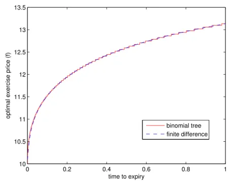
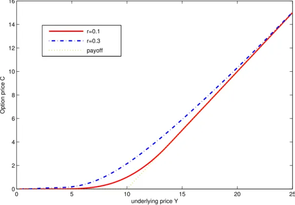
Depicted in Fig 3.2 is the comparison between the optimal exercise price pro-duced by the current scheme withN = 10000,I = 300,J = 20 and the binomial tree method with N = 10000. We focus on the calculation of the optimal exercise price because it is far more difficult to be calculated accurately than the option price [37]. As observed from Fig 3.2, the optimal exercise price calculated by the two methods agree well with each other. Precisely, the maximum point-wise error is no more than 0.89%. In Fig 3.3, we further display the option price C as a function of underlying
Y at two interest rate levels. Clearly, the option price is an increasing function of underlying, which conforms the financial clause set for a standard American call. Moreover, the smooth pasting condition across the free boundary is well satisfied at both interest rate levels. These test results also confirm the reliability of the current method.
Figure 3.2: Comparison of the solutions produced by the current scheme and the binomial tree method. Model parameters are r = 0.1, σ1 = 0.3, σ2 = 0,
ρ=−0.1,γ = 0.1,D= 0.1,K= 10, T = 1. 0 0.2 0.4 0.6 0.8 1 10 10.5 11 11.5 12 12.5 13 13.5 time to expiry
optimal exercise price (f)
binomial tree finite difference
3.3.2
Quantitative analysis
With confidence in the current scheme, we investigate the relationship betweent interest rate and the optimal exercise price. Impacts of parameters ρ and σ2 on
stock loans are studied. Since what solved in the last section is C, we first find the values ofV and Sf by (3.7). Notice that the optimal exercise price of the stock loan plotted here is a function of τ.
Figure 3.3: Option price with different interest rate values. Model parameters areσ1= 0.3,σ2= 0.2, ρ=−0.5, γ= 0.1, D= 0.1,K = 10, T = 2. 0 5 10 15 20 25 0 2 4 6 8 10 12 14 16 underlying price Y Option price C r=0.1 r=0.3 payoff
plot the boundary against the interest rate at T = 0. A relating question is that whether the optimal exercise boundary is higher for different levels of interest rate. As observed from Fig 3.4, the optimal exercise price is an increasing function of the interest rate at a fixed time point. To confirm the conclusion that the optimal exercise price is higher with a higher interest rate level (not only at a fixed time point), we plotted three boundary optimal exercise boundaries in Fig 3.5. From this additional figure we find that the optimal price is indeed higher with a higher interest rate level.
Figure 3.4: The optimal exercise boundary of stock loan. Model parameters are
σ1 = 0.3,σ2 = 0.2,γ = 0.1,D= 0.1,K = 10,T = 2. 0 0.1 0.2 0.3 0.4 0.5 0.6 0.7 0.8 0.9 1 10 20 30 40 50 60 70 80 90 100 Interest rate
Optimal exercise price
Now we turn to investigate impacts of other parameters. Depicted in Fig 3.6 are optimal exercise boundaries of stock loans at r = 0.1 with three σ2 values. We
observe that the optimal exercise price is higher with a larger value of σ2.
Consid-ering that σ2 = 0 represents the constant interest, we conclude that the stochastic
interest rate leads to a higher optimal exercise price. Financially, it means that the investor demands a larger compensation since the interest rate with a higher volatility is more attractive.
Financially, a lower correlation between interest rate and stock price means that low stock prices come with higher interest rates [30]. As a result, it is more attractive to hold the call option. In a nutshell, a smallerρindicates a higher optimal exercise price of the American call option. Since f(τ, r) = e−γtSf(t, r), there should be the same result when it comes to the stock loan with stochastic interest rate. Depicted in Fig 3.7 are optimal exercise prices of stock loan with differentρvalue withrbeing
Figure 3.5: Optimal exercise boundaries of stock loan at different interest levels. Model parameters