Self-Adaptive Workload Classification and Forecasting
for Proactive Resource Provisioning
Nikolas Roman Herbst
Karlsruhe Institute of Technology Am Fasanengarten 5 76131 Karlsruhe, Germany
Nikolaus Huber
Karlsruhe Institute of Technology Am Fasanengarten 5 76131 Karlsruhe, GermanySamuel Kounev
Karlsruhe Institute of Technology Am Fasanengarten 5 76131 Karlsruhe, GermanyErich Amrehn
IBM Research & Development Schoenaicher Str. 220 71032 Boeblingen, Germany
[email protected]
ABSTRACT
As modern enterprise software systems become increasingly dynamic, workload forecasting techniques are gaining in im-portance as a foundation for online capacity planning and resource management. Time series analysis offers a broad spectrum of methods to calculate workload forecasts based on history monitoring data. Related work in the field of workload forecasting mostly concentrates on evaluating spe-cific methods and their individual optimisation potential or on predicting Quality-of-Service (QoS) metrics directly. As a basis, we present a survey on established forecasting methods of the time series analysis concerning their benefits and drawbacks and group them according to their compu-tational overheads. In this paper, we propose a novel self-adaptive approach that selects suitable forecasting methods for a given context based on a decision tree and direct feed-back cycles together with a corresponding implementation. The user needs to provide only his general forecasting objec-tives. In several experiments and case studies based on real-world workload traces, we show that our implementation of the approach provides continuous and reliable forecast re-sults at run-time. The rere-sults of this extensive evaluation show that the relative error of the individual forecast points is significantly reduced compared to statically applied fore-casting methods, e.g. in an exemplary scenario on average by 37%. In a case study, between 55% and 75% of the viola-tions of a given service level agreement can be prevented by applying proactive resource provisioning based on the fore-cast results of our implementation.
Permission to make digital or hard copies of all or part of this work for personal or classroom use is granted without fee provided that copies are not made or distributed for profit or commercial advantage and that copies bear this notice and the full citation on the first page. To copy otherwise, to republish, to post on servers or to redistribute to lists, requires prior specific permission and/or a fee.
ICPE’13,April 21–24, 2013, Prague, Czech Republic. Copyright 2013 ACM 978-1-4503-1636-1/13/04 ...$15.00.
Categories and Subject Descriptors
C.4 [Computer Systems Organization]: Performance of
Systems
Keywords
workload forecasting, arrival rate, time series analysis, pro-active resource provisioning
1.
INTRODUCTION
Virtualization allows to dynamically assign and release re-sources to and from hosted applications at run-time. The amount of resources consumed by the executed software services are mainly determined by the workload intensity. Therefore, they both typically vary over time according to the user’s behavior. The flexibility that virtualization en-ables in resource provisioning and the variation of the resource demands over time raise a dynamic optimisation -problem. Mechanisms that continuously provide appropri-ate solutions to this optimisation problem could exploit the potential to use physical resources more efficiently resulting in cost and energy savings as discussed for example in [1, 23].
Commonly, mechanisms that try to continuously match the amounts of demanded to provisioned resources are reac-tive as they use threshold based rules to detect and react on resource shortages. However, such reactive mechanisms can be combined with proactive ones that anticipate changes in resource demands and proactively reconfigure the system to avoid resource shortages. For building such proactive mech-anisms, the time series analysis offers a spectrum of sophis-ticated forecasting methods. But as none of these methods is the best performing in general, we work on the idea to in-telligently combine the benefits of the individual forecasting methods to achieve higher forecast accuracy independent of the forecasting context.
In this paper, we present a survey of forecasting meth-ods offered by the time series analysis that base their com-putations on periodically monitored arrival rate statistics. We group the individual forecasting methods according to
their computational overhead, their benefits and drawbacks as well as their underlying assumptions. Based on this anal-ysis, we design a novel forecasting methodology that dynam-ically selects at run-time a suitable forecasting method for a given context. This selection is based on a decision tree that captures the users’ forecasting objectives, requirements of individual forecasting methods and integrates direct feed-back cycles on the forecast accuracy as well as heuristics for further optimisations using data analysis. Users need to provide only their general forecast objectives concern-ing forecastconcern-ing frequency, horizon, accuracy and overhead and are not responsible to dynamically select appropriate forecasting methods. Our implementation of the proposed Workload Classification and Forecasting (WCF) approach is able to continuously provide time series of point forecasts of the workload intensity with confidence intervals and forecast accuracy metrics in configurable intervals and with control-lable computational overhead during run-time.
In summary, the contributions of this paper are: (i) We identify the characteristics and components of an observed workload intensity behavior and define metrics to quantify these characteristics for the purpose of automatic classifica-tion and selecclassifica-tion of a forecasting method. (ii) We provide a survey of state-of-the-art forecasting approaches based on time series analysis (including interpolation, decomposition and pattern identification techniques) focusing on their ben-efits, drawbacks and underlying assumptions as well as their computational overheads. (iii) We propose an novel forecast-ing methodology that self-adaptively correlates workload in-tensity behavior classes and existing time series based fore-casting approaches. (iv) We provide an implementation of
the proposed WCF approach as part of a new
Workload-ClassificationAndForecasting(WCF) system1
specifical-ly designed for online usage. (v) We evaluate our WCF ap-proach using our implementation in the context of multiple different experiments and case studies based on real-world workload intensity traces.
The results of our extensive experimental evaluation con-sidering multiple different scenarios show that the dynamic selection of a suitable forecast method significantly reduces the relative error of the workload forecasts compared to the results of a statically selected fixed forecasting method, e.g. in the presented exemplary scenario on average by 37%. Even when limiting the set of forecasting methods consid-ered in the dynamic selection, our self-adaptive approach achieves a higher forecast accuracy with less outliers than individual methods achieve in isolation. In the presented case study, we apply proactive resource provisioning based on the forecast results of the introduced WCF approach and achieve to prevent between 55% and 75% of the violations of a given service level agreement (SLA).
The major benefit of our self-adaptive WCF approach is an enhancement in foresight for any system that is capable of dynamically provision its resources. In other words, our WCF approach is able to extend the reconfiguration times a system needs for its optimisation. Additionally, the forecast results that are provided by the WCF system can be used for anomaly detection.
The remainder of the paper is structured as follows: In Section 2, we define several concepts and terms that are cru-cial for understanding the presented approach. In the next
1
http://www.descartes-research.net/tools/
step, we analyze characteristics of a workload intensity be-havior and give a compact survey on existing workload fore-casting methods based on time series analysis. We present our self-adaptive approach for workload classification and forecasting in Section 3. In Section 4, we evaluate the WCF approach by presenting and discussing an exemplary exper-iment and a case study. We review related work in Section 5, and present some concluding remarks in Section 6.
2.
FOUNDATIONS
In this section, we start by defining crucial terms in the context of software services, workload characterization and performance analysis that are helpful to build a precise un-derstanding of the presented concepts and ideas and are used in the rest of the paper:
We assume thatSoftware services are offered by a
com-puting system to a set of users which can be humans or other systems. In our context, a software service can be seen as a deployed software component.
EachRequest submitted to the software service by a user encapsulates an individual usage of the service.
Arequest class is a category of requests that are charac-terized by statistically indistinguishable resource demands.
Aresource demand in units of time or capacity is a mea-sure of the consumption of physical or virtual resources in-curred for processing an individual request.
The termworkload refers to the physical usage of the
sys-tem over time comprising requests of one or more request classes. This definition deviates from the definition in [29],
where workload is defined as a more general term
captur-ing in addition to the above the respective applications and their SLAs.
Aworkload categoryis a coarse-grained classification of a workload type with respect to four basic application and technology domains as defined in [29]: (i) Database and Transaction Processing, (ii) Business Process Applications, (iii) Analytics and High Performance Computing, (iv) Web Collaboration and Infrastructures.
A time series X is a discrete function that represents
real-valued measurements xi ∈ R for every time point ti
in a set of n equidistant time pointst=t1, t2, ..., tn: X =
x1, x2, ..., xnas described in [26]. The elapsed time between
two points in the time series is defined by a value and a time unit.
The number of time series points that add up to the next upper time unit or another time period of interest is called thefrequency of a time series. The frequency attribute of a time series is an important starting point for the search of seasonal patterns.
Atime series of request arrival ratesis a time series whose
values representni ∈N unique request arrivals during the
corresponding time intervals [ti, ti+1).
A workload intensity behavior (WIB) is a description of a workload’s characteristic changes in intensity over time like the shape of seasonal patterns and trends as well as the level of noise and bursts as further described in the following section. The WIB can be extracted from a corresponding time series of request arrival rates.
2.1
Workload Intensity Behavior
According the theory of the time series analysis [8, 16, 28], a time series can be decomposed into the following three
components, whose relative weights and shapes characterise the respective WIB:
The trend component can be described by a monotoni-cally increasing or decreasing function (in most cases a linear function) that can be approximated using common
regres-sion techniques. A break within the trend component is
caused by system extrinsic events and therefore cannot be forecast based on historic observations but detected in retro-spect. It is possible to estimate the likelihood of a change in the trend component by analysing the durations of historic trends.
The season component captures recurring patterns that are composed of at least one or more frequencies, e.g. daily, weekly or monthly patterns (but they do not need to be integer valued). These frequencies can be identified by using a Fast Fourier Transformation (FFT) or by auto-correlation techniques.
Thenoise component is an unpredictable overlay of var-ious frequencies with different amplitudes changing quickly due to random influences on the time series. The noise can be reduced by applying smoothing techniques like weighted moving averages (WMA), by using lower sampling frequency, or by a low-pass filter that eliminates high frequencies. Find-ing a suitable trade-off between the amount of noise reduc-tion and the respective potential loss of informareduc-tion can en-hance forecast accuracy.
A time series decomposition into the above mentioned components is illustrated in Figure 1. This decomposition of a time series has been presented in [31]. The authors offer an implementation of their approach for time series deposition and detection of breaks in trends or seasonal
com-ponents (BFAST)2. In the first row, the time series input
data is plotted. The second row contains detected (yearly) seasonal patterns, whereas the third row shows estimated trends and several breaks within these trends. The remain-der in the unremain-dermost row is the non-deterministic noise com-ponent computed by the difference between the original time series data and the sum of the trend and the seasonal com-ponents. ð òé ð ð òè ð ð òçð ¼ ¿ ¬¿ ó ð òð ì ð òð ð ð òðì -»¿ -± ² ¿´ ð òé ê ð òèî ¬® » ²¼ ó ð òð ë ð òðë îððð îððî îððì îððê îððè ®» ³ ¿ ·² ¼ »® Ì·³»
Figure 1: Time Series Decomposition into Season, Trend and Noise Components as presented in [31]
The theory of time series analysis differentiates between static and dynamic stochastic processes. In static process models, it is assumed that the trend and season component remain constant, whereas in dynamic process models, these
2
http://bfast.r-forge.r-project.org/
components change or develop over time and therefore have to be approximated periodically to achieve good quality fore-casts. Still, the trend and season components are considered to be deterministic and the quality of their approximation is important for the workload forecasting techniques. Depend-ing on the applied stochastic model, the season, trend and noise components can be considered either as multiplicative or additive.
A nearly complete decomposition of a time series into the three components described above using for example the BFAST approach [31] induces a high computational over-head. Hence, more easily computable characteristics of a time series are crucial for efficient workload classification at run-time as described in the following:
Theburstiness index is a measure for the spontaneity of fluctuations within the time series and calculated by the ratio of the maximum observed value to the median within a sliding window.
Thelength of the time series mainly influences the accu-racy of approximations for the above mentioned components and limits the space of applicable forecasting methods.
The number ofconsecutive monotonic values either
up-wards or downup-wards within a sliding window indirectly char-acterises the influence of the noise and seasonal components. A respective small value can be seen as a sign of a high noise level and a hint to apply a time series smoothing technique. Themaximum, themedian and thequartiles are impor-tant indicators of the distribution of the time series data and
can be unified in the quartile dispersion coefficient (QDC)
defined as the distance of the quartiles divided by the me-dian value.
The standard deviation and the mean value are combined
in thecoefficient of variation(COV) which characterizes the
dispersion of the distribution as a dimensionless quantity. Absolutepositivityof a time series is an important charac-teristic because intervals containing negative or zero values can influence the forecast accuracy and even the applicabil-ity of certain forecasting methods. As arrival rates cannot be negative by nature, a time series that is not absolutely positive should be subjected to a simple filter eliminating the negative values or analyzed using specialized forecasting method.
We define arelative gradient as the absolute gradient of
the latest quarter of a time series period in relation to the
median of this quarter. It captures the steepness of the
latest quarter period as a dimensionless value. A positive relative gradient shows that the last quarter period changed less than the median value, a negative value indicates a steep section within the time series (e.g., the limb of a seasonal pattern).
Thefrequency of a time series represents the number of
time series values that form a period of interest (in most
cases simply the next bigger time-unit). These values are an important input as they are used as starting points for the search for seasonal patterns.
The presented metrics are sufficient to capture the most important characteristics of a WIB, though they have low computational complexity. Hence, they are of major impor-tance for our online workload classification process.
2.2
Survey of Forecasting Methods
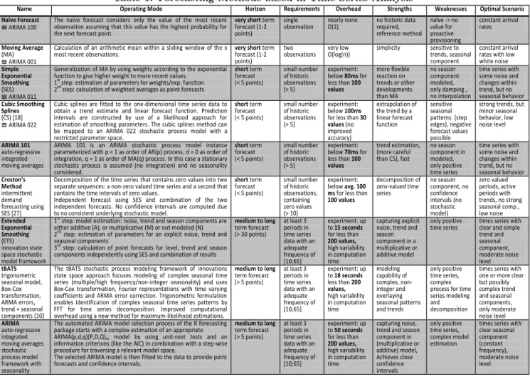
In this section, we compare the most common forecasting approaches based on the time series analysis and highlight
Table 1: Forecasting Methods based in Time Series Analysis
Name Operating Mode Horizon Requirements Overhead Strengths Weaknesses Optimal Scenario Naïve Forecast
≘ ARIMA 100
The naïve forecast considers only the value of the most recent observation assuming that this value has the highest probability for the next forecast point.
very short term forecast (1-2 points)
single
observation nearly none O(1) no historic data required, reference method naïve -> no value for proactive provisioning constant arrival rates Moving Average (MA) ≘ ARIMA 001
Calculation of an arithmetic mean within a sliding window of the x
most recent observations. very shortforecast (1-2 term points)
two
observations very low O(log(n)) simplicity sensitive to trends, seasonal component
constant arrival rates with low white noise Simple Exponential Smoothing (SES) ≘ ARIMA 011
Generalization of MA by using weights according to the exponential function to give higher weight to more recent values.
1st
step: estimation of parameters for weights/exp. function 2nd step: calculation of weighted averages as point forecasts
short term forecast (< 5 points) small number of historic observations (> 5) experiment: below 80ms for less than 100 values more flexible reaction on trends or other developments than MA no season component modeled, only damping , no interpolation
time series with some noise and changes within trend, but no seasonal behavior Cubic Smoothing Splines (CS) [18] ≘ ARIMA 022
Cubic splines are fitted to the one-dimensional time series data to obtain a trend estimate and linear forecast function. Prediction intervals are constructed by use of a likelihood approach for estimation of smoothing parameters. The cubic splines method can be mapped to an ARIMA 022 stochastic process model with a restricted parameter space.
short term forecast (< 5 points) small number of historic observations (> 5) experiment: below 100ms
for less than 30 values (no improved accuracy) extrapolation of the trend by a linear forecast function sensitive seasonal patterns (step edges), negative forecast values possible
strong trends, but minor seasonal behavior, low noise level ARIMA 101 auto-regressive integrated moving averages
ARIMA 101 is an ARIMA stochastic process model instance parameterized with p = 1 as order of AR(p) process, d = 0 as order of integration, q = 1 as order of MA(q) process. In this case a stationary stochastic process is assumed (no integration) and no seasonality considered. short term forecast (< 5 points) small number of historic observations (> 5) experiment: below 70ms for less than 100 values trend estimation, (more careful than CS), fast no season component in modeled, only positive time series
time series with some noise and changes within trend, but no seasonal behavior Croston’s Method intermittent demand forecasting using SES [27]
Decomposition of the time series that contains zero values into two separate sequences: a non-zero valued time series and a second that contains the time intervals of zero values.
Independent forecast using SES and combination of the two independent forecasts. No confidence intervals are computed due to no consistent underlying stochastic model.
short term forecast (< 5 points) small number of historic observations, containing zero values (> 10) experiment: below avg. 100 ms for less than
100 values decomposition of zero-valued time series no season component, no confidence intervals (no stochastic model) zero valued periods, active periods with trends, no strong seasonal comp., low noise Extended Exponential Smoothing (ETS) innovation state space stochastic model framework 1st
step: model estimation: noise, trend and season components are either additive (A), or multiplicative (M) or not modeled (N) 2nd
step: estimation of parameters for an explicit noise, trend and seasonal components
3rd
step: calculation of point forecasts for level, trend and season components independently using SES and combination of results
medium to long term forecast (> 30 points) at least 3 periods in time series data with an adequate frequency of [10;65] experiment: up to 15 seconds
for less than
200 values,
high variability in computation time
capturing explicit noise, trend and season component in a multiplicative or additive model
only positive
time series times series with clear and simple trend and seasonal component, moderate noise level tBATS trigonometric seasonal model, Box-Cox transformation, ARMA errors, trend + seasonal components [10]
The tBATS stochastic process modeling framework of innovations state space approach focuses modeling of complex seasonal time series (multiple/high frequency/non-integer seasonality) and uses Box-Cox transformation, Fourier representations with time varying coefficients and ARMA error correction. Trigonometric formulation enables identification of complex seasonal time series patterns by FFT for time series decomposition. Improved computational overhead using a new method for maximum-likelihood estimations.
medium to long term forecast (> 5 points) at least 3 periods in time series data with an adequate frequency of [10;65] experiment: up to 18 seconds less than 200 values, high variability in computation time modeling capability of complex, non-integer and overlaying seasonal patterns and trends only positive time series, complex process for time series modeling and decomposition
times series with one or more clear but possibly complex trend and seasonal components, only moderate noise level ARIMA auto-regressive integrated moving averages stochastic process model framework with seasonality
The automated ARIMA model selection process of the R forecasting package starts with a complex estimation of an appropriate ARIMA(p,d,q)(P,D,Q)m model by using unit-root tests and an
information criterions (like the AIC) in combination with a step-wise procedure for traversing a relevant model space.
The selected ARIMA model is then fitted to the data to provide point forecasts and confidence intervals.
medium to long term forecast (> 5 points) at least 3 periods in time series data with an adequate frequency of [10;65] experiment: up to 50 seconds
for less than
200 values,
high variability in computation time
capturing noise, trend and season component in (multiplicative or additive) model, Achieves close confidence intervals only positive time series, complex model estimation
times series with clear seasonal component (constant frequency), moderate noise level
their requirements, advantages and disadvantages present-ing a short summary based on [8, 16, 17, 28, 10, 18, 27]. All considered forecasting methods have been implemented
by Hyndman in the R forecast package3 and documented
in [17]. The implemented forecasting methods are based ei-ther on the state-space approach [16] or the ARIMA (auto-regressive integrated moving averages) approach for stochas-tic process modelling [8]. These two general approaches for stochastic process modeling have common aspects, but are not identical as in both cases there exist model instances that have no counterpart in the other approach and both have different strength and weaknesses as discussed, e.g., in [17]. In Table 1, we briefly describe the considered forecasting approaches which are ordered according to their computa-tional complexity. Besides from [17], detailed information on the implementation, parameters and model estimation of the individual methods can be taken from cited sources within Table 1. Capturing the complexity in common O-notation in most cases is infeasible except for the two first simple cases. As the shape of seasonal patterns contained in the data as well as the used optimisation thresholds during a model fitting procedure strongly influence the computa-tional costs, the length of time series size represents only one part of the problem description. Therefore, the
compu-3
http://robjhyndman.com/software/forecast/
tational complexity of the individual methods has been eval-uated based on experiments with a representative amount of forecasting method executions on a machine with a
In-tel Core i7 CPU (2.7 GHz). The forecasting methods make
use of only a single core as multi-threading is not yet fully supported by the existing implementations.
2.3
Forecast Accuracy Metrics
A number of error metrics have been proposed to capture the differences between point forecasts and corresponding
observations. They are summarized, explained and
com-pared in [19]. The authors propose to use theMean Absolute
Scaled Error (MASE) as forecast accuracy metric to enable consistent comparisons of forecasting methods across
differ-ent data samples. The MASE metric for an interval [m, n] is
defined as follows withb[m,n] as the average change within
the observation:
(I)errort=f orecastt−observationt, t∈[m, n]
(II)b[m,n]= n−1m·
Pn
i=m+1|observationi−observationi−1|
(III)M ASE[m, n] =meant=[m+1,n]( errort b[m,n] )
Computing the MASE metric enables direct interpretation whether the forecast accuracy is higher compared to the naive forecasting approach which typically serves as a ref-erence. Therefore, we use the MASE metric as the central
element to build a reliable and direct feedback mechanism for our WCF approach as presented in the following section.
3.
APPROACH
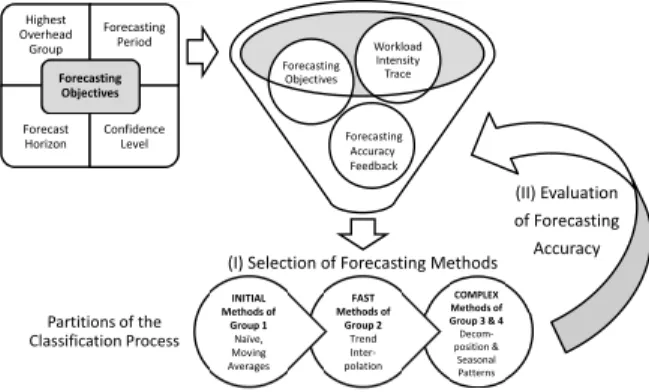
As stated in the Introduction, the major contribution of this paper is the construction of an online workload clas-sification mechanism for optimized forecasting method se-lection. In this section, we present the individual concepts that are incorporated into our WCF approach as sketched in Figure 2. Highest Overhead Group Forecasting Period Forecast Horizon Confidence Level
Forecasting Objectives
(I) Selection of Forecasting Methods
Forecasting Objectives Workload Intensity Trace INITIAL Methods of Group 1 Naïve, Moving Averages Partitions of the Classification Process (II) Evaluation of Forecasting Accuracy Forecasting Accuracy Feedback FAST Methods of Group 2 Trend Inter-polation COMPLEX Methods of Group 3 & 4 Decom-position & Seasonal Patterns
Figure 2: Workload Classification Process
We will use the term WIB class to refer to the current
choice of the most appropriate forecasting method. Each class identifier is equal to the name of the corresponding forecasting method. A WIB may change and develop over time in a way that the classification is not stationary and therefore it needs to be periodically updated. The WIB class
at a time pointtcorresponds to the currently selected
fore-casting methodAproviding the best accuracy compared to
the other available forecasting methods. At a later point in
timet+i, the WIB may be reclassified and may now
cor-respond to another forecasting methodB. As in some cases
different forecasting methods may possibly deliver identical results, the class of a WIB is not necessarily unique at each point in time.
3.1
Overhead of Forecasting Methods
The forecasting methods as presented in Table 1 are grou-ped into four subsets according to their computational over-head:
Group 1 stands for nearly no overhead and contains the Moving Average (MA)and theNaive forecasting methods.
Group 2 stands for low overhead and contains the fast
forecasting methodsSimple Exponential Smoothing (SES),
Cubic Spline Interpolation (CS), the predefinedARIMA101
model and the specializedCroston’s Methodfor intermittent
time series. The processing times of forecasting methods in
this group are below 100msfor a maximum of 100 time series
points.
Group 3 stands for medium overheads and contains the
forecasting methodsExtended Exponential Smoothing (ETS)
andtBATS. The processing times are below 30 seconds for less than 200 time series points.
Group 4 stands for high overheads and contains again tBATS and additionally theARIMAforecasting framework
with automatic selection of an optimalARIMAmodel. The
processing times remain below 60 seconds for less than 200 time series points.
3.2
Forecasting Objectives
Given that forecast results can be used for a variety of pur-poses like manual long term capacity planning or short term proactive resource provisioning, a set of forecasting objec-tives is introduced to enable tailored forecast result process-ing and overhead control. The followprocess-ing parameters charac-terizing the forecasting objectives are defined:
(i) TheHighest Overhead Group parameter is a value of
the interval [1,4] specifying the highest overhead group from which the forecasting methods may be chosen in the classi-fication process.
(ii) TheForecast Horizonparameters are defined as a
tu-ple of two positive integer values quantifying the number of time series points to forecast. The first value defines the start value, the second value accordingly the maximum fore-cast horizon setting. Due to the significant differences of the forecasting methods in term of their processing times and capabilities for long term forecasts, the start value need to be increased up to the given maximum value during the learning phase (until the periods are contained in the time series data) using multipliers that are defined as part of the configuration of the classification process.
(iii) TheConfidence Levelparameter can be a value in the
interval [0,100) and sets the confidence levelalphaas per-centage for the confidence intervals surrounding the forecast mean values.
(iv)Forecasting Period is a positive integer parameter i
specifying how often in terms of the number of time series points a forecasting method execution is triggered. The con-figuration of the presented parameters allows to customize the forecasting strategy according to the characteristics of the considered scenario.
3.3
Partitions of the Classification Process
We partition the classification process according to the amount of historic data available in the time series to sup-port an initial partition, a fast partition and a complex parti-tion. These partitions are connected to the overhead groups of the forecasting methods. Having a short time series, only
forecasting methods in theoverhead group 1 can be applied.
A medium length may allow application of methods
con-tained in the overhead group 2 and a long time series
en-ables the use of the methods in overhead group 3 and 4.
The two thresholds that define when a time series is short, medium or long can be set as parameters in the classifica-tion setting. Based on experience gained from experiments, it is our recommendation to set the initial-fast threshold to a value between five (as this is the minimal amount of point needed for Cubic Spline Interpolation) and the value corresponding to half a period. The fast-complex threshold should be set to a value as high as covering three complete time series periods for the simple reason that most methods in the respective overhead group need at least three pattern occurrences to identify them.
3.4
Optional Smoothing
A high noise level within thetime series of request arrival ratescomplicates every forecasting process. To improve the forecast accuracy it is conducive to observe metrics that
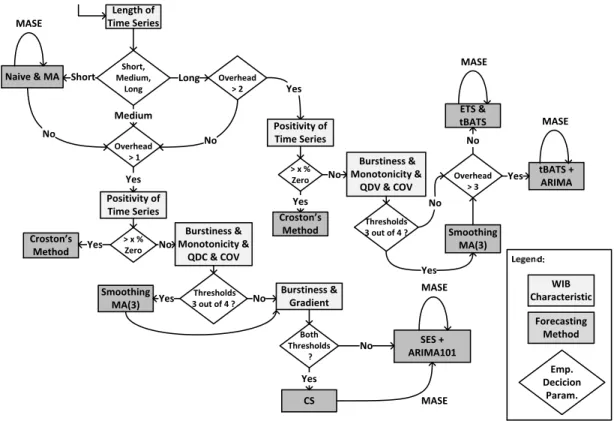
cap-Length of Time Series Short, Medium, Long Short Overhead > 1 SES + ARIMA101 No tBATS + ARIMA ETS & tBATS WIB Characteristic Forecasting Method Emp. Decicion Param. Naive & MA MASE Medium Overhead > 2 Long No Positivity of Time Series Yes > x % Zero Croston’s Method Yes No Burstiness & Monotonicity & QDC & COV No Thresholds 3 out of 4 ? Smoothing MA(3) Yes MASE Yes > x % Zero Croston’s Method Yes Positivity of Time Series Overhead > 3 No No Burstiness & Monotonicity & QDV & COV Thresholds 3 out of 4 ? Smoothing MA(3) Yes Yes No MASE MASE Burstiness & Gradient Both Thresholds ? CS Yes MASE No
Figure 3: Decision Tree for Online Classification and Selection of Appropriate Forecasting Methods
ture the noise level within the time series and define thresh-olds to trigger a smoothing method before the time series is processed by the forecasting method. However, any smooth-ing method has to be applied carefully not to eliminate valu-able information. The four metrics (burstiness index, rela-tive monotonicity, COV and QDC) introduced in Section 2.1 are suitable and sufficient to quantify noise related char-acteristics within a time series and therefore are repeatedly applied to the set of the most recent time series points of
configurable lengthn. Smoothing of the time series can be
achieved for example using the elementary method Weighted Moving Averages (WMA) where the level of smoothing can easily be controlled by the window size and the weights. In our WCF approach, we observe the four mentioned noise-related metrics and apply WMA when three of them cross configurable thresholds. We use a window size of three, a weight vectorw= (0.25,0.5,0.25) and a control variable to assure that no time series value is smoothed more than one time. With this setting we are carefully smooth out a high noise level, but avoid the loss of valuable information. Time series smoothing can also be achieved by far more complex methods like using a Fast Fourier Transformation to build a low-pass filter eliminating high frequencies. However, this would introduce additional overheads and would require an inadequately high amount of time series data.
3.5
Decisions based on Forecast Accuracy
As mentioned in Section 2.3 and extensively discussed in [19], the MASE metric is the metric of choice for quan-tifying the forecast accuracy. We describe in this Section
how the MASE metric is used in our adaptive classification process to identify and validate the current WIB class.
Given that the MASE metric compares the forecast accu-racy against the accuaccu-racy of the naive forecasting method, it is directly visible when a method performs poorly. If the MASE value is close to one or even bigger, the computed forecast results are of no value, as their accuracy is equal or even worse than directly using monitoring values. The closer the metric value is to zero, the better the forecast-ing method delivers trustworthy forecast results. The fore-casting method having the smallest MASE value defines the WIB class of our adaptive classification process.
In our approach, two or more forecasting methods are ex-ecuted in parallel and compared in configurable intervals to check whether the recent WIB class is still valid. This WIB class validation is also triggered when the forecast result
seems implausible or shows low accuracy (MASE value>1).
The MASE metric is estimated during the forecast execution itself as at this point in time observation values are not yet available. This estimation needed when two or more fore-casting methods are executed in parallel to output the more promising result. Just before the next forecast execution is triggered, the MASE metric is then precisely calculated as observation values and forecast results are available at this point in time and used to validate the WIB classification.
3.6
Decision Tree with Feedback Cycles
The presented concepts and mechanisms were combined to build our WCF approach that automatically adapts to changing WIBs with the result of optimized and more con-stantly adequate forecasting accuracy. The combination of
a classification process with a set of forecasting methods enables a configuration according to given forecasting ob-jectives. Figure 3 illustrates the classification process of the WCF approach. The classification process can be seen as independent from the forecasting method executions and is triggered according to the configuration of theclassification period parameter every n time series points, just before a forecasting method execution is requested. The classifica-tion process uses the forecasting objectives specified by the user and the WIB characteristics to reduce the space of pos-sible forecasting methods. The suitable forecasting meth-ods are then processed together and their estimated fore-cast accuracy is evaluated to output the more promising result. Before the next forecasting method execution, the classification (which is the selection of the better perform-ing method) is validated by the observed MASE metric and used until the next classification process execution is trig-gered. The WCF parameter set we propose in this section follows rules of thumb from time series analysis literature and has been experimentally calibrated using several inde-pendent real-world workload traces provided by IBM. These traces are not used for the evaluation of the WCF approach. In the presented exemplary scenario and the case study in Section 4 the recommended parameter set is applied with-out any changes. For further case specific optimisations, the WCF approach can be controlled in detail by adjusting the parameter settings and thresholds.
4.
EVALUATION
In this section, we present results of an extensive evalu-ation of our WCF approach based on real-world scenarios. Due to the space constraints, we focus on presenting a se-lected experiment focusing a forecast accuracy comparison and an exemplary case study where the forecast results are interpreted for proactive resource provisioning. In general, real-world WIB traces are likely to exhibit strong seasonal patterns with daily periods due to the fact that the users of many software services are humans. The daily seasonal patterns are possibly overlaid by patterns of a longer periods such as weeks or months. Depending on the monitoring pre-cision, a certain noise level is normally observed, but can be reduced by aggregation of monitoring intervals or smoothing techniques as discussed in Section 3.4. Deterministic bursts within a WIB trace are often induced by planned batch tasks (for example in transaction processing systems). In addition, a WIB trace can exhibit non-deterministic bursts that can-not be foreseen by any time series analysis technique due to system extrinsic influences. For the evaluation of the WCF approach we used multiple real-world WIB traces with dif-ferent characteristics representing difdif-ferent types of work-loads. The results presented in this paper are based on the following two WIB traces:
(i)Wikipedia Germany Page Requests: The hourly num-ber of page requests at the webpage of Wikipedia Germany
has been extracted from the publicly available server logs4
for October 2011.
(ii)CICStransaction processing monitoring data was
pro-vided by IBM of an real-world deployment of an IBM z10 mainframe server. The data reports the number of started transactions during one week from Monday to Sunday in 30 minute windows.
4
http://dumps.wikimedia.org/other/pagecounts-raw/
4.1
Exemplary Scenario
In the presented exemplary scenario, the WCF system uses forecasting methods from all four overhead groups and is compared to the fixed use of the Extended Exponential
Smoothing (ETS) method. Additionally, the Naive
fore-casting method (which is equivalent to system monitoring without forecasting) is compared to the other forecasting methods to quantify and illustrate the benefit of applying forecasting methods against just monitoring the request ar-rival rates. The individual forecasting methods have been executed with identical exemplary forecast objectives on the same input data and are therefore reproducible. The fore-cast results are provided continuously over the experiment duration, which means that at the end of an experiment there is for every observed request arrival rate a correspond-ing forecast mean value with a confidence interval. This al-lows to evaluate whether the WCF system successfully clas-sifies the WIB. A successful classification would mean that the forecasting method that delivers the highest accuracy for a particular forecasting interval is selected by the WCF system. To quantify the forecast result accuracy, a relative error is calculated for every individual forecast mean value:
relativeErrort= |f orecastV alueobservedArrivalRatet−observedArrivalRatet|
t .
The distributions of these relative errors are illustrated us-ing cumulative histograms which have inclusive error classes on the x-axis and the corresponding percentage of all
fore-cast points on the y-axis. In other words, an [x, y] tuple
expresses that y percent of the forecast points have a
rela-tive error between 0% andx%. Accordingly, given that the
constant liney= 100% represents the hypothetical optimal
error distribution, in each case the topmost line represents the best case of the compared alternatives with the lowest error. We chose to illustrate the error distribution using cu-mulative histograms to obtain monotone discrete functions of the error distribution resulting in less intersections and therefore in a clearer illustration of the data. To improve readability, the histograms are not drawn using bars but sim-ple lines connecting the individual [x, y] tuples. In addition, statistical key indices like the arithmetic mean, the median and the quartiles as well as the maximum were computed to enable direct comparison of the relative error distribu-tions and rank the forecasting methods according to their achieved forecast accuracy. Finally, directed paired t-tests from common statistics were applied to ensure the statis-tical significance of the observed differences in the forecast accuracy of the different forecasting methods.
This experiment compares the forecast accuracy of the WCF approach with the ETS method and the Naive method during a learning process which means that at the beginning there is no historical data available to the individual casting methods that are compared. Concerning the fore-casting objectives, the forecast horizon (in this scenario iden-tical to the forecasting frequency) for all forecasting methods is configured to increase stepwise as shown in Table 2. The maximum overhead group is set to 4 for an unrestricted set of forecasting methods. The confidence level is set to 95%, but not further interpreted in this scenario.
The cumulative error distribution for each of the meth-ods are shown in Figure 5 as well as in Figure 6 which demonstrate that the WCF method achieves significantly better forecast accuracy compared to ETS and Naive. ETS can only partially achieve slightly better forecast accuracy than the Naive method, however, it induces processing
over--100 0 100 200 300 400 500
NAIVE NAIVE NAI
VE NAI VE NAI VE NAI VE AR IM A101 CS CS AR IM A1 01 CS SES SES AR IM A101 AR IM A1 01 AR IM A1 01 AR IM A1 01 AR IM A101 AR IM A101 CS CS CS CS CS CS AR IM A1 01 AR IM A1 01 AR IM A1 01 AR IM A101 AR IM A101 AR IM A101 CS CS CS CS SES AR IM A AR IM A AR IM A AR IM A AR IM A AR IM A TB ATS TB ATS TB ATS AR IM A AR IM A AR IM A TB ATS TB ATS TB ATS TBAT S TBAT S TB ATS AR IM A AR IM A AR IM A AR IM A AR IM A AR IM A 01234567891011121314151617181920212223242526272829303132333435363738394041424344454647484950515253545556575859606162636465666768697071727374757677787980818283 84 85 86 87 88 89 90 91 1 0 0 0 x CI CS t ran sacti ons per 3 0 min ut e in terv al ETS WCF Observation Monday Tuesday Wednesday Thursday Friday
classification by WCF
# forecast execution -> overhead group 2, horizon 2 -> overhead group 4, horizon 12
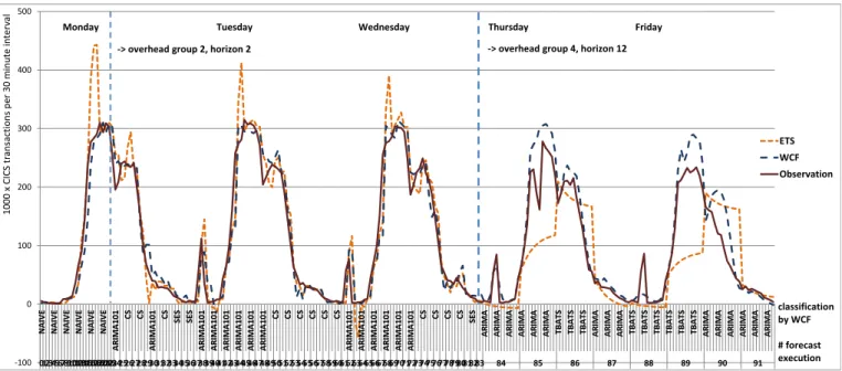
Figure 4: Exemplary Scenario: Comparison Chart of WCF and ETS
Table 2: Exemplary Scenario
Experiment Focus Comparison of unrestricted WCF to static ETS and Naive Forecasting Methods WCF(1-4), ETS(3), Naive(1) (overhead group)
Input Data CICS transactions, Monday to Friday, WIB trace 240 values in transactions per 30 minutes,
frequency = 48, 5 periods as days Forecast Horizon (h) h = 1 for 1sthalf period,
(= Forecasting Frequency) h = 2 until 3rdperiod complete,
h = 12 for 4thand 5thperiod
heads of 715 ms per forecasting method execution compared to 45 ms for the Naive method (computation of the confi-dence intervals). The WCF method has an average process-ing overhead of 61 ms durprocess-ing the first three periods of the WIB trace. For the fourth and fifth period (Thursday and Friday), when forecasting methods of the overhead group 4 are selected, WCF’s processing overhead per forecasting method execution is on average 13.1 seconds. The forecast mean values of the individual methods and the respective actual observed request arrival rates in the course of time are plotted in Figure 4. In this chart it is visible that the ETS method forecast values have several bursts during the first three periods and therefore do not remain as close to the actual observed values as the WCF forecast values do. During the last eight forecast executions the WCF approach successfully detects the daily pattern early enough to achieve better results than ETS.
The WCF approach shows the lowest median error value of 20.7% and the lowest mean error value of 47.4%. In addi-tion, WCF has a significantly smaller maximum error value. Though the ETS method is a sophisticated procedure on its own, the results of the presented exemplary scenario demon-strate that the application of ETS on its own leads to poor
5% 10% 15% 20% 25% 30% 35% 40% 45% 50% 55% 60% 65% 70% 75% 80% 85% 90% 95%100% > Naive 10% 19% 23% 28% 34% 41% 46% 49% 51% 56% 59% 62% 67% 68% 69% 71% 79% 80% 85% 87%100% ETS 12% 19% 30% 36% 43% 46% 50% 53% 56% 61% 63% 66% 71% 73% 74% 75% 76% 79% 79% 81%100% WCF 13% 25% 34% 46% 56% 64% 66% 68% 70% 72% 76% 79% 82% 82% 83% 86% 88% 89% 90% 91%100% 0% 10% 20% 30% 40% 50% 60% 70% 80% 90% 100% p er cen t of f ore cas t v alu es
Cumulative Percentage Error Distribution
Comparison of WCF to ETS and Naive forecasting methods CICS transactions (5 days, 48 frequency, 240 forecast values)
percentage error class [0%, x%]
Figure 5: Exemplary Results: Cumulative Error
Distribution of WCF, ETS and Naive
forecast accuracy with average errors almost as high as for the Naive method and even higher maximal errors.
4.2
Case Study
In this section, we present a case study demonstrating how the proposed WCF method can be successfully used for proactive online resource provisioning. WCF offers a higher degree of flexibility due to the spectrum of integrated
fore-WCF
ETS
Naiv
e
0.0 0.5 1.0 1.5
Figure 6: Exemplary Results: Box & Whisker Plots of the Error Distributions
0 0,5 1 1,5 2 2,5 3 3,5 4 NAI VE NAI VE NAI VE CS CS CS CS CS CS SES A R IM A 10 1 CS CS CS SE S TB A T S TB A T S A R IM A A R IM A A R IM A A R IM A A R IM A A R IM A A R IM A A R IM A A R IM A A R IM A A R IM A A R IM A A R IM A A R IM A A R IM A TB A T S TB A T S A R IM A A R IM A A R IM A A R IM A A R IM A A R IM A A R IM A A R IM A A R IM A A R IM A A R IM A A R IM A A R IM A A R IM A * ** *** TBA T S TB A T S TB A T S A R IM A A R IM A A R IM A A R IM A A R IM A A R IM A A R IM A TBA T S TB A T S A R IM A A R IM A A R IM A A R IM A A R IM A A R IM A A R IM A 012345678910111213141516171819202122232425262728293031 32 33 34 35 36 37 38 39 40 41 42 43 44 45 *** 60 61 62 63 64 65 66 67 M ill io n Wi ki p e d ia Page R e q u e sts p e r h o u rs upper confidence lower confidence forecasted value observation upper threshold lower threshold Day 1 Monday classification by WCF # forecast execution Day 8 Monday Day 18 Thursday
-> overhead group 2, horizon 3
//
-> overhead group 4, horizon 12
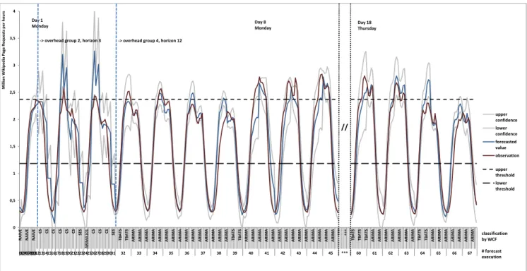
Figure 7: Case Study Chart: 21 Days Wikipedia Page Requests, WCF4 approach
cast methods. None of these forecasting methods can offer this degrees of flexibility on their own. For this case study scenario, there is no historic knowledge available at the be-ginning and the WCF has to adapt to this and wait for the first three periods (Monday, Tuesday, Wednesday) until fore-casting methods of the overhead group 4 can be applied. For an arrival rate higher than a given threshold, the SLA of the average response time is violated. We assume that the un-derlying system of the analyzed workload intensity behavior is linearly scalable from zero to three server instances. This assumption implies a constant average resource demand per request for all system configurations. Furthermore we as-sume the presence of a resource provisioning system that reacts on observed SLA violations as well as on forecast re-sults. For an arrival rate lower than a given threshold, the running server instances are not efficiently used and there-fore one of them is shut down or put in stand by mode. In this scenario, the WCF system provides forecast mean values and confidence intervals to the resource provisioning system which then can proactively add or remove server instances at that point in time, when the resource or server is needed, in addition to solely reacting on SLA violations. Details on the WCF configuration for this case study scenario are given in Table 3.
In Figure 7, the WCF forecast values are plotted together with the corresponding confidence intervals and the actual observed workload intensities. The two dotted lines repre-sent the given thresholds that define when a server instance needs to be started or shut down. The upper threshold is placed in a way that it is not reached constantly in every daily seasonal period (for example not on the weekends). The additions or removals of server instances are triggered either in a reactive manner after an SLA violation or in a
Table 3: Case Study Scenario
Forecast Strategy WCF(1-4) (overhead group)
Input Data Wikipedia Germany, 3 weeks, WIB trace 504 values in page requests per hour,
frequency = 24, 21 periods as days Forecast Horizon h = 1 for 1st
half period (= Forecasting Frequency) h = 3 until 3rdperiod is complete (number of forecast points (h)) h = 12 from 4th
on Confidence Level 80 %
proactive fashion anticipating the points in time when SLA violations would occur. It can be seen that SLA violations cannot be forecast reliably in the first three daily periods. For the following daily periods, SLA violations can be cor-rectly anticipated in the majority of cases. Only when the amplitude of the daily pattern changes, for example before and after weekends, the forecast mean values deliver false positives or do not anticipate the need for additional com-puting resources on time. To obtain the results summarized
Table 4: Case Study: SLA Violations Summary
Comparison Reactive vs. proactive WCF based
provisioning of server instances
Reactive 76 SLA violations
Proactive 42 SLA violations correctly anticipated
(WCF based) and 15 more nearly correctly
6 cases of false positives
in Table 4, we counted correct, incorrect and nearly correct forecasts for all threshold crossings of the real workload. In the worst case 34 and in the best case 19 SLA violations occur when using the proactive approach based on WCF compared to 76 SLA violations in the reactive case. 17% of SLA violations were not anticipated by the proactive WCF-based approach in addition to 8% reported false positives.
4.3
Result Interpretation
As part of our comprehensive evaluation, we considered a number of different scenarios under different workloads with different forecasting objectives and different respective WCF configurations. The experiment results show that the WCF system is able to sensitively select appropriate forecasting methods for particular contexts thereby improving the over-all forecast accuracy significantly and reducing the number of outliers as compared to individual forecasting methods applied on their own. In the presented exemplary scenario, WCF achieved an improvement in forecast accuracy on av-erage by 37%. As demonstrated in the case study scenario, the interpretation of WCF forecast results by proactive re-source provisioning reduces the number of SLA violations by between 55% to 75%. In addition, our proposed self-adaptive WCF approach supports the system users to select a forecasting method according to their forecasting objec-tives. Especially at the beginning of a WIB’s lifetime, when no or few historical data is available, a static decision made by a user would not fit for the WIB’s lifetime. With its dy-namic design and the flexibility to react on changes in the WIB, the WCF system is able to adapt to such changes, thereby increasing the overall accuracy of the forecast re-sults. Our WCF system enables online and continuous fore-cast processing with controllable computational overheads. We achieve this by scheduling forecasting method execu-tions and WIB classificaexecu-tions in configurable periods. In all experiments, the processing times of all forecasting meth-ods remained within the boundaries specified by their cor-responding overhead group in such a way that the forecast results are available before their corresponding request ar-rival rates are monitored. The latter is crucial especially for the execution of forecasting methods at a high frequency with short horizons.
For a WIB with strong daily seasonal pattern and high amplitude variance due to known calendar effects, the fore-cast accuracy might be strongly improved by splitting this WIB into two separate time series: regular working days in the first and weekends and public holidays in the second. This can reduce the impact of the possibly strong overlay of weekly patterns. As part of our future work, we plan to introduce support for such time series splittings as well as for the selection of the data aggregation level for varying forecasting objectives. This can be achieved by a realisation of an intelligent filter applied to the monitoring data before it is provided to the WCF system in form of time series.
5.
RELATED WORK
We divide related work into the following three groups: (i) The first group of related work has its focus on evaluating forecasting methods applied to either workload related data or performance monitoring data. (ii) In the second group of related work we consider approaches for workload fore-casting that are not based on the methods of the time series analysis, as opposed to our proposed WCF approach.
(iii) In the third group of related work we cover research that has its focus on approaches for proactive resource pro-visioning using tailored forecasting methods.
(i) In 2004, Bennani and Menasc´e have published their
re-search results of an robustness assessment on self-managing computer systems under highly variable workloads [4]. They come to the conclusion that proactive resource management improves a system’s robustness under highly variable
work-loads. Furthermore, the authors compare three different
trend interpolating forecasting methods (polynomial inter-polation, weighted moving averages and exponential smooth-ing) that have been introduced as means for workload
fore-casting in [24]. Bennani and Menasc´e propose to select the
forecasting methods according to the lowestR2 error as
ac-curacy feedback. Still, the focus of this work is more on the potentials of proactive resource provisioning and the evalu-ation of forecasting methods is limited to basic trend inter-polation methods without any pattern recognition for sea-sonal time series components. In [11], Frotscher assesses the capabilities to predict response times by evaluating the fore-cast results provided by two concrete ARIMA models with-out seasonality, simple exponential smoothing (SES) and the Holt-Winters approach as a special case of the extended ex-ponential smoothing (ETS). His evaluation is based on gen-erated and therefore possibly unrealistic times series data. The author admits that the spectrum of forecasting meth-ods offered by time series analysis is not covered and he is critical about the capability to predict response times of the evaluated methods as their strengths in trend extrapolation does not suit to typically quickly alternating response times. (ii) In [21] and a related research paper [5], the authors propose to use neuronal nets and machine learning approa-ches for demand prediction. This demand predictions are meant to be used by an operating system’s resource man-ager. Goldszmidt, Cohen and Powers use an approach based on Bayesian learning mechanisms for feature selection and short term performance forecasts described in [13]. Short-coming of these approaches is that the training of the ap-plied neuronal nets on a certain pattern need to be com-pleted before the nets can provide pattern based forecasts. This stepwise procedure limits the flexibility and implies the availability of high amounts of monitoring data for the min-ing of possibly observable patterns.
(iii) The authors of [12] use a tailored method to decom-pose a time series into its dominating frequencies using a Fourier transformation and then apply trend interpolation techniques to finally generate a synthetic workload as fore-cast. Similarly in [14], Fourier analysis techniques are ap-plied to predict future arrival rates. In [9], the authors base their forecast technique on pattern matching methods to de-tect non-periodic repetitive behavior of cloud clients. The research of Bobroff, Kochut and Beaty presented in [7] has its focus on the dynamic placement of virtual machines, but workload forecasting is covered by the application of static
ARMA processes for demand prediction. In [20], an
ap-proach is proposed and evaluated that classifies the gradi-ents of a sliding window as a trend estimation on which the resource provisioning decision are then based. The au-thors Grunske, Aymin and Colman of [3, 2] focus on QoS forecasting such as response time and propose an automated and scenario specific enhanced forecast approach that uses a combination of ARMA and GARCH stochastic process mod-eling frameworks for frequency based representation of time
series data. This way, the authors achieve improved fore-cast accuracy for QoS attributes that typically have quickly alternating values. In [25], different methods of the time se-ries analysis and Bayesian learning approaches are applied. The authors propose to periodically selected a forecasting method using forecast accuracy metrics. But it is not fur-ther evaluated how significantly this feedback improves the overall forecast accuracy. No information is given on how the user’s forecast objectives are captured and on how the computational overheads can be controlled. In contrast to our research, the authors concentrate on the prediction of resource consumptions.
However, besides of [25], a common limitation of the above mentioned approaches is their focus on individual methods that are optimised or designed to cover a subset of typical situations. Therefore, they are not able to cover all pos-sible situations adequately as it could be achieved by an intelligent combination of the innovation state space frame-works (ETS and tBATS) and the auto-regressive integrated moving averages (ARIMA) framework for stochastic process modeling. Furthermore, in all mentioned approaches besides in [14], the resource utilisation or average response times are monitored and taken as an indirect metric for the recent workload intensity. But these QoS metrics are indirectly in-fluenced by the changing amounts of provisioned resources and several other factors. The forecasting computations are then based on these values that bypass resource demand esti-mations per request and interleave by principle performance relevant characteristics of the software system as they can be captured in a system performance model.
6.
CONCLUSION
Today’s resource managing systems of virtualized comput-ing environments often work solely reactive uscomput-ing threshold-based rules, not leveraging the potential of proactive re-source provisioning to improve a system performance while maintaining resource efficiency. The results of our research is a step towards exploiting this potential by computing con-tinuous and reliable forecasts of request arrival rates with appropriate accuracy.
The basis of our approach was the identification of work-load intensity behavior specific characteristics and metrics that quantify them. Moreover, we presented a survey on the strengths, weaknesses and requirements of existing forecast methods from the time series analysis and ways to estimate and evaluate the forecast accuracy of individual forecast ex-ecutions. As the major contribution of this paper, we pre-sented an approach classifying workload intensity behaviors to dynamically select appropriate forecasting methods. This has been achieved by using direct feedback mechanisms that evaluate and compare the recent accuracy of different fore-casting methods. They have been incorporated into a deci-sion tree that considers user specified forecasting objectives. This enables online application and processing of continu-ous forecast results for a variable number of different WIBs. Finally, we evaluated an implementation of our proposed ap-proach in different experiments and an extensive case study based on different real-world workload traces. Our exper-iments demonstrate that the relative error of the forecast points in relation to the monitored request arrival rates is significantly reduced as in the exemplary scenario by 37% on average compared to the results of a static application of the Extended Exponential Smoothing (ETS) method. More
importantly, the major benefit of our approach has been demonstrated in an extensive case study, showing how it is possible to prevent between 55% and 75% of SLA violations.
6.1
Future Work
We plan to extend the functionality of the WCF system to apply it in further areas. One extension is the combina-tion of the WCF system with an intelligent filter that helps a system user to fit the aggregation level of the monitored arrival rates for specific forecasting objectives, e.g, continu-ous short term forecasts for proactive resource allocation or manually triggered long term forecasts for server capacity planning. For divergent forecasting objectives, such a fil-ter would multiplex an input stream of monitoring data and provide it as individual WIBs in different aggregation levels at the data input interface of the WCF system. A second WCF system application area will be a combination with an anomaly detection system like ΘPAD as outlined in [6] at the data output interface of the WCF system. Such a sys-tem can compute continuous anomaly ratings by comparing the WCF system’s forecast results with the monitored data. The anomaly rating can serve to analyze the workload in-tensity behavior for sudden and unforeseen changes and in addition as an reliability indicator of the WCF system’s re-cent forecast results.
Ultimately, we will connect the WCF system’s interface (data input) to a monitoring framework like Kieker [30] to continuously provide online forecast results. These forecast results can then be used as input for self-adaptive resource management approaches like [15], giving them the ability to proactively adapt the system to changes in the work-load intensity. This combination of workwork-load forecasting and model-based system reconfiguration is an important step to-wards the realization of self-aware systems [22].
7.
REFERENCES
[1] H. Abdelsalam, K. Maly, R. Mukkamala, M. Zubair, and D. Kaminsky. Analysis of energy efficiency in
clouds. InFuture Computing, Service Computation,
Cognitive, Adaptive, Content, Patterns, 2009. COMPUTATIONWORLD ’09. Computation World:, pages 416–421, nov. 2009.
[2] A. Amin, A. Colman, and L. Grunske. An Approach to Forecasting QoS Attributes of Web Services Based
on ARIMA and GARCH Models. InProceedings of the
19th IEEE International Conference on Web Services (ICWS). IEEE, 2012.
[3] A. Amin, L. Grunske, and A. Colman. An Automated Approach to Forecasting QoS Attributes Based on Linear and Non-linear Time Series Modeling. In (Accepted for publication to appear) Proceedings of the 27th IEEE/ACM International Conference on Automated Software Engineering (ASE). IEEE/ACM, 2012.
[4] M. N. Bennani and D. A. Menasce. Assessing the robustness of self-managing computer systems under
highly variable workloads. InProceedings of the First
International Conference on Autonomic Computing, pages 62–69, Washington, DC, USA, 2004. IEEE Computer Society.
[5] M. Bensch, D. Brugger, W. Rosenstiel, M. Bogdan, W. G. Spruth, and P. Baeuerle. Self-learning
prediction system for optimisation of workload management in a mainframe operating system. In ICEIS, pages 212–218, 2007.
[6] T. C. Bielefeld. Online Performance Anomaly Detection for Large-Scale Software Systems, March 2012. Diploma Thesis, University of Kiel.
[7] N. Bobroff, A. Kochut, and K. Beaty. Dynamic placement of virtual machines for managing sla
violations. InIntegrated Network Management, 2007.
IM ’07. 10th IFIP/IEEE International Symposium on, pages 119 –128, 21 2007-yearly 25 2007.
[8] G. Box, G. Jenkins, and G. Reinsel.Time series
analysis : forecasting and control. Wiley series in probability and statistics. Wiley, Hoboken, NJ, 4. ed. edition, 2008. Includes index.
[9] E. Caron, F. Desprez, and A. Muresan. Pattern matching based forecast of non-periodic repetitive
behavior for cloud clients.J. Grid Comput., 9:49–64,
March 2011.
[10] A. M. De Livera, R. J. Hyndman, and R. D. Snyder. Forecasting time series with complex seasonal patterns
using exponential smoothing.Journal of the American
Statistical Association, 106(496):1513–1527, 2011. [11] T. Frotscher. Prognoseverfahren f¨ur das
Antwortzeitverhalten von Software-Komponenten,
March 2011. Christian-Albrechts-Universit¨at zu Kiel,
Bachelor’s Thesis.
[12] D. Gmach, J. Rolia, L. Cherkasova, and A. Kemper. Workload analysis and demand prediction of
enterprise data center applications. InProceedings of
the 2007 IEEE 10th International Symposium on Workload Characterization, IISWC ’07, pages 171–180, Washington, DC, USA, 2007. IEEE Computer Society. [13] M. Goldszmidt, I. Cohen, and R. Powers. Short term
performance forecasting in enterprise systems. InIn
ACM SIGKDD Intl. Conf. on Knowledge Discovery and Data Mining, pages 801–807. ACM Press, 2005. [14] M. Hedwig, S. Malkowski, C. Bodenstein, and
D. Neumann. Towards autonomic cost-aware allocation of cloud resources. InProceedings of the International Conference on Information Systems ICIS 2010, 2010.
[15] N. Huber, F. Brosig, and S. Kounev. Model-based Self-Adaptive Resource Allocation in Virtualized
Environments. In6th International Symposium on
Software Engineering for Adaptive and Self-Managing Systems (SEAMS 2011), Honolulu, HI, USA, May 23-24 2011.
[16] R. Hyndman, A. K¨ohler, K. Ord, and R. Snyder,
editors.Forecasting with Exponential Smoothing : The
State Space Approach. Springer Series in Statistics. Springer-Verlag Berlin Heidelberg, Berlin, Heidelberg, 2008.
[17] R. J. Hyndman and Y. Khandakar. Automatic time series forecasting: The forecast package for R, 7 2008. [18] R. J. Hyndman, M. L. King, I. Pitrun, and B. Billah. Local linear forecasts using cubic smoothing splines. Monash Econometrics and Business Statistics Working Papers 10/02, Monash University, Department of Econometrics and Business Statistics, 2002. [19] R. J. Hyndman and A. B. Koehler. Another look at
measures of forecast accuracy.International Journal of
Forecasting, pages 679–688, 2006.
[20] H. Kim, W. Kim, and Y. Kim. Predictable cloud provisioning using analysis of user resource usage patterns in virtualized environment. In T.-h. Kim, S. S. Yau, O. Gervasi, B.-H. Kang, A. Stoica, and
D. Slezak, editors,Grid and Distributed Computing,
Control and Automation, volume 121 of Communications in Computer and Information Science, pages 84–94. Springer Berlin Heidelberg, 2010.
[21] S. D. Kleeberg. Neuronale Netze und Maschinelles
Lernen zur Lastvorhersage in z/OS. Universit¨at
T¨ubingen, Diploma Thesis.
[22] S. Kounev, F. Brosig, N. Huber, and R. Reussner. Towards self-aware performance and resource management in modern service-oriented systems. In Proceedings of the 2010 IEEE International Conference on Services Computing, SCC ’10, pages 621–624, Washington, DC, USA, 2010. IEEE Computer Society.
[23] L. Lef`evre and A.-C. Orgerie. Designing and
evaluating an energy efficient cloud.The Journal of
Supercomputing, 51:352–373, 2010. 10.1007/s11227-010-0414-2.
[24] D. A. Menasc´e and V. A. F. Almeida.Capacity
planning for Web performance: metrics, models, and methods. Prentice-Hall, Inc., Upper Saddle River, NJ, USA, 1998.
[25] X. Meng, C. Isci, J. Kephart, L. Zhang, E. Bouillet, and D. Pendarakis. Efficient resource provisioning in
compute clouds via vm multiplexing. InProceedings of
the 7th international conference on Autonomic computing, ICAC ’10, pages 11–20, New York, NY, USA, 2010. ACM.
[26] T. Mitsa.Temporal Data Mining. Chapman &
Hall/CRC data mining and knowledge discovery series. Chapman & Hall/CRC, 2009.
[27] L. Shenstone and R. J. Hyndman. Stochastic models underlying croston’s method for intermittent demand forecasting.Journal of Forecasting, 24(6):389–402, 2005.
[28] R. H. Shumway.Time Series Analysis and Its
Applications : With R Examples. Springer Texts in StatisticsSpringerLink : B¨ucher. Springer
Science+Business Media, LLC, New York, NY, 2011. [29] J. Temple and R. Lebsack. Fit for Purpose: Workload
Based Platform Selection. Technical report, IBM Corporation, 2010.
[30] A. van Hoorn, J. Waller, and W. Hasselbring. Kieker: A framework for application performance monitoring
and dynamic software analysis. InProceedings of the
3rd ACM/SPEC International Conference on Performance Engineering (ICPE 2012). ACM, Apr. 2012. Invited tool demo paper. To appear.
[31] J. Verbesselt, R. Hyndman, A. Zeileis, and D. Culvenor. Phenological change detection while accounting for abrupt and gradual trends in satellite
image time series.Remote Sensing of Environment,
![Figure 1: Time Series Decomposition into Season, Trend and Noise Components as presented in [31]](https://thumb-us.123doks.com/thumbv2/123dok_us/1123201.2649618/3.918.94.430.718.910/figure-series-decomposition-season-trend-noise-components-presented.webp)