Semiparametric Estimation of the Bid-Ask Spread in Extended
Roll Models
Xiaohong Chena∗ Oliver Lintonb† Stefan Schneebergerc‡ Yanping Yid § aCowles Foundation for Research in Economics, Yale University
b Department of Economics, University of Cambridge cDepartment of Economics, Yale University
dSchool of Economics, Shanghai University of Finance and Economics
First version: August 2015; Revised November 22, 2017
Abstract
We propose new methods for estimating the bid-ask spread from observed transaction prices alone. Our methods are based on the empirical characteristic function. We compare our meth-ods theoretically and numerically with the Roll (1984) method as well as with its best known competitor, the Hasbrouck (2004) method, and find that our estimators perform much better when this distribution is far from Gaussian. Our methods are applied to the E-mini futures con-tract on the S&P 500 during the Flash Crash of May 6, 2010. We also establish√T consistency and asymptotic normality of the proposed estimators in various extended Roll models.
JEL Classification Number: C12, C13, C14.
Keywords: Bid-ask spread; Roll model; Semiparametric estimation; Empirical characteristic func-tion; Latent variables.
∗
PO Box 208281, New Haven CT 06520-8281, USA. E-mail: [email protected].
†
Austin Robinson Building, Sidgwick Avenue, Cambridge CB3 9DD, UK. E-mail: [email protected].
‡
New Haven CT 06520-8281, USA. E-mail: [email protected].
§
The corresponding author. Tel.: (+86)21-65902962. Address : School of Economics, Shanghai University of Finance and Economics, 777 Guoding Road, Shanghai, 200433, China. E-mail: [email protected].
1
Introduction
The bid-ask spread of a financial asset is the difference between the ask and the bid quotes. The spread reflects the cost of providing market liquidity, the difference in price paid by an urgent buyer
and received by an urgent seller, which is a major part of the transaction cost facing investors. It has
been studied extensively by financial economists, see, e.g. Glosten and Milgrom (1985), Glosten and Harris (1988), Harris (1990), Huang and Stoll (1997), Schultz (2001), Harris and Piwowar (2006),
Corwin and Schultz (2012), Bleaney and Li (2015), and the references therein. The estimation strategy of the bid-ask spread (transaction cost) depends crucially on the market structure andthe data availability.
Measuring the bid-ask spread in practice can be quite time consuming (reconstruction of the
limit order book is required) and may be subject to a number of potential accuracy issues due to the quoting strategies of High Frequency Traders, for example. For the U.S. municipal bond market
(see, e.g., Harris and Piwowar (2006)) and the U.S. corporate bond market (see, e.g., Edwards et al.
(2007)), the firm bid and ask quotes are absent. As for other over-the-counter (OTC) markets, market-wide transaction data are generally not available (see, e.g., Jankowitsch et al. (2011)). Data
are also limited for open outcry markets (e.g. the futures trading in CME), where bid and ask quotes by traders expire (if not filled) without recording (see, e.g., Hasbrouck (2004)). Moreover, in
the U.S. markets transaction data are only available since 1983and in many countries transaction data are not available at all.
Using observed transaction prices alone, the seminal paper Roll (1984) proposes a simple model to estimate the effective bid-ask spread without information on the bid and the ask quotes, or the
trade direction (i.e., whether the trade initiator is a buyer or a seller). The basic Roll estimator has seen its popularity in analyzing the U.S. historical data sets (prior to 1983), the international
markets without transaction data, the illiquid markets (particularly OTC markets), the cases when
intraday quotes and trades cannot be reliably matched, and the cases when the transaction data are cumbersome to use or expensive to purchase.
In the Roll (1984) model, an observed (log) asset price pt evolves according to pt=p∗t +It s0 2, p ∗ t =p∗t−1+εt, (1) ∆pt=εt+ (It−It−1) s0 2 =εt+ ∆It s0 2 , (2)
where{p∗t} are the underlying fundamental (log) price with serially uncorrelated innovations{εt}. The trade direction indicators {It} are i.i.d. and take the values +1 (if the transaction is buyer initiated), or−1 (if the transaction is seller initiated) with equal probability. {εt}are uncorrelated with {It}. Essentially, Roll (1984) assumes an informationally efficient market. The parameter of interest s0 is the effective bid-ask spread, measuring the order processing cost. The transaction
prices{pt}are the only observable variables in Eq.(1). Thus, assuming the one-period returns{∆pt} have finite second moments, the true unknowns0 is identified using the population auto-covariance
of {∆pt} and can be estimated using its sample analogue
s0= 2
p
−Cov(∆pt,∆pt−1), bsRoll:= 2 q
−Covd(∆pt,∆pt−1). (3)
In practice, this estimator is not satisfactory, since the empirical first-order autocovariance of
one-period returns is often positive, then Eq.(3) is not well-defined. Roll (1984) encounters this phe-nomenon in about a half of the cases in his data, which consists of annual samples of daily and
weekly prices. The literature contains several proposals to deal with this shortcoming. Harris (1990)
suggests to replace−Covd(∆pt,∆pt−1) in (3) by its absolute value
Covd(∆pt,∆pt−1) . This makes
the estimator always well-defined. Hasbrouck (2009) suggests to set the estimated spread to zero if
the empirical autocovariance is positive, which is motivated by the finding of Harris (1990) that pos-itive autocovariance estimates are more likely for smaller spreads. However, it is not clear whether
either of these ad hoc modifications work well in finite samples, and they are theoretically not well motivated.
A well-known alternative by Hasbrouck (2004) proposes to estimate the bid-ask spread based on Bayesian analysis, using the Gibbs sampler. In doing so, he uses a stronger version of the Roll model,
in whichεt ∼i.i.d. N 0, σ2ε
jointly with the spreads0. Unfortunately the Hasbrouck (2004) estimator performs poorly or even
is not well defined when the distribution of εt is far from Gaussian, e.g. fat-tailed or asymmetric. However, the Gaussian assumption generally fails in financial data. Corwin and Schultz (2012)
develop another spread estimator from consecutive daily high and low transaction prices. They also assume that the fundamental price process is a geometric Brownian motion, which is even stronger
than the discrete time Gaussian assumption employed in Hasbrouck (2004).
The recent empirical literature emphasizes several issues with the Roll model : (a) Market
orders are assumed not to bring news into prices, so that It has no effect on the underlying true price p∗t. However, the literature finds the quoted prices increase after a buyer-initiated trade (see, e.g., Glosten and Milgrom (1985), Glosten and Harris (1988), Huang and Stoll (1997), Muravyev
(2016)). (b) It assumes balanced market order flow, i.e.,q= 1/2,which may be accurate on average, but may be inaccurate for certain episodes of trading (see, e.g., Brunnermeier and Pedersen (2005),
Ito and Yamada (2016)). (c) It assumes always a price change due to transactions, but many transactions might happen with no price change (see, e.g., Huang and Stoll (1997)). In the presence
of any of these effects, one is not able to identify the spread jointly with parameters describing adverse selection cost or order flow imbalance, using either Roll (1984)’s or Hasbrouck (2004)’s
methodology, without additional assumptions or observed information. The spread estimators of
Roll (1984) and Hasbrouck (2004) will also be inconsistent. There have been many recent suggestions for estimating spreads (and liquidity costs more generally), that relax some of these assumptions,
but at the cost of requiring additional observed information (data) such as trade direction indicators. As we have mentioned, these data may not be readily available or, if available, be not well measured
for the relevant frequency (see, e.g., Andersen and Bondarenko (2014)). Bleaney and Li (2015) provide a detailed discussion of all the above and additional problems with the basic Roll (1984)
model. Goyenko et al. (2009) review many different liquidity proxies based on lower frequency data, including the Roll-type transaction-price-based measures, as well as those that use additional
information such as trading volumes.
transaction prices are available. These prices could be daily or weekly closing prices, but might also consist of high frequency intraday prices. However, contrary to, e.g., Corwin and Schultz (2012), we do not require intraday data for our method to work. We assume that{εt}is i.i.d. and independent of the increments of the unobserved trade direction indicators {∆It}, or independent of{It} when adverse selection cost is considered. The independence assumption allows us to propose new, simple
estimators ofs0 that are based on empirical characteristic functions. However, we do not impose any
parametric restrictions (in contrast to Hasbrouck (2004)), or any location/scale assumptions, and
we do not require the existence of moments of any order (in contrast to Roll (1984), which requiresεt to have finite second moments). This feature seems to be attractive for financial applications where distributions can be asymmetric and heavy-tailed. In addition to the basic Roll (1984) model, we
also propose solutions to the three problems (a)-(c) with the Roll model listed above. We show how to estimate parameters that capture an adverse selection component in the spread in Section 3, or
those associated with unbalanced order flow in Section 4, or those that characterize the probability of no price change in Section 5. The consistency and asymptotic normality of our estimators are
established without requiring finite moments of the observed price data. In simulation studies that mimic the design of Hasbrouck (2009), our estimators are competitive to Roll (1984)’s and
Hasbrouck (2004)’s when the latent true fundamental return distribution is Gaussian, and perform
much better when the distribution is either asymmetric or heavy-tailed.
We apply our estimators to a high-frequency dataset of transaction prices on the E-mini futures
contract during the Flash Crash of May 6, 2010. We use a rolling-window approach to understand the development of the spread during the crisis period and more tranquil periods. In the
applica-tion, we also show the evolution of some additional estimated quantities, including the estimated characteristic function of the fundamental price innovationsεt, indicators for an unbalanced order flow, an adverse selection component in the spread, and the aggregation robustness of our method. The rest of the paper is organized as follows: Section 2 presents the basic model and provides new
simple spread estimators and their asymptotic properties. In Section 3, we study the estimation of adverse selection cost. In Section 4, we address order flow imbalance in a simple extended
model. In Section 5, a simplified model is used to consider the case when the transaction may occur
without price change. Section 6 presents a simulation study and the empirical application. Section 7 concludes. All the proofs, some figures and tables are presented in the online supplement.
2
Basic Model and Large Sample Properties of Estimators
In this section we assume that the observed price dynamics follow a basic Roll (1984) type model.
Assumption 1. (i) Data {pt}Tt=1 is generated from Eq. (1) with s0 >0, where {εt} is i.i.d. and
independent of{∆It}and has unknown distribution function F; (ii){It}is i.i.d.; and (iii) It takes
the values ±1 with equal probability.
The distribution of εt could be continuous or discrete and could have no finite moments. Let ϕε(u) := E(exp (iuεt)) denote the characteristic function (c.f.) of εt. Let ϕ∆p,2(u, u0) := E(exp (iu∆pt+iu0∆pt−1)) and ϕ∆p,1(u) :=E(exp (iu∆pt)) =ϕ∆p,2(u,0)denote the joint c.f. of
(∆pt,∆pt−1) and the marginal c.f. of ∆pt, respectively. By definition, they are nonparametrically identified and estimable from data. We shall obtain a useful expression based on these quantities that will identify the unknown spread parameter s0 > 0. The use of marginal quantities such
as characteristic functions for identification of s0 is reminiscent of the classic GMM approach to
identification and estimation of continuous time models where the transition density is hard to
ex-press analytically, but many moment conditions can be obtained from the marginal distributions. Precisely, Assumption 1 implies that, for all (u, u0)∈R2,
ϕ∆p,2(u, u0) =ϕε(u)ϕε(u0) cos us0 2 cos(u0−u)s0 2 cosu0s0 2 . (4)
If the distribution of εt were parametrically specified, one could work directly with equation (4) and develop estimation methods that would be a simple alternative to the Hasbrouck (2004)
likelihood-type procedure. In our case, where this distribution is not specified, these relations still involve the unknown function ϕε, albeit in a convenient multiplicative fashion. We find a relation that eliminates the unknown functionϕε(·),and then proceed to estimate the parametric model for
the trade direction effects0. Denote
V :={u∈R:ϕ∆p,1(u)6= 0}. (5)
Sinceϕ∆p,1(·) is uniformly continuous inR(see, e.g., page 3 of Lukacs (1972)) andϕ∆p,1(0) = 1, V
contains an open interval of01. Denote
H(u, u0) := ϕ∆p,2(u, u 0)
ϕ∆p,1(u)ϕ∆p,1(u0)
f or any (u, u0)∈ V2, (6)
which is nonparametrically estimable from the data{∆pt}. Eq. (4) implies that
H(u, u0) = cos (u−u 0)s0 2 cos us0 2 cos u0s0 2 =:R(u, u 0 ;s0) f or all (u, u0)∈ V2, (7)
and therefore H(u, u0) is real-valued for all (u, u0)∈ V2. Or equivalently,
ϕ∆p,2(u, u0) =ϕ∆p,1(u)ϕ∆p,1(u0)R(u, u0;s0) f or all(u, u0)∈ V2. (8)
Eq. (7) (or (8)) is free of the nuisance functionϕε(·)and only depends on the parameter of interest
s0. Chen et al. (2017) obtains the identification result for s0 and the c.f. ϕε(·) using either the diagonal information or the off-diagonal information of Eq. (7) (or (8)).
Eq. (7) (or (8)) for estimation of s0 is similar to the classic GMM approach to estimation. Due
to the continuity of the c.f. ϕ∆p,2(u, u0) in R2 and ϕ∆p,2(0,0) = 1, V2 contains an open ball of
(0,0), and hence Eq. (7) (or (8)) contains infinitely many overidentifying restrictions for s0. Let
S := [0, s]denote the parameter space, where s >0 is chosen from prior experience for the market (to ensure thats0 ∈ S). Denote
U := (u, u0)∈ V2 : min s∈S cos us 2 cosu0s 2 >0 , (9)
which still contains an open ball of(0,0). Denote
R(u, u0;s) := cos (u−u 0)s 2 cos us2 cos u0s 2 , (10)
which is well defined on U × S. Let U ⊆ U and |U |denote the number of points inU, which can be chosen such that|U | ≥1. We introduce two simple minimum distance criterion functions on S:2
J(s,U) := X (u,u0)∈U |ϕ∆p,2(u, u0)−ϕ∆p,1(u)ϕ∆p,1(u0)R(u, u0;s)|2 ≥0, (11) Q(s,U) := X (u,u0)∈U |H(u, u0)−R(u, u0;s)|2≥0, (12) where| · |denotes the modulus of a complex number. Since Eq. (7) (or (8)) holds for all(u, u0)∈ V2
and U ⊆ U ⊆ V2, both criteria are minimized ats=s
0, i.e.,J(s0,U) = 0 andQ(s0,U) = 0. Assumption 2. (i)s0∈ S, whereS is compact; (ii)U ⊆ U, and∃(˜u,u˜)∈ U such thatu˜∈(0, π/s);
and (iii) |U |<∞.
As shown in Theorem 3 of Chen et al. (2017), under Assumption 1 and 2, s0 is identified as
the unique solution tomins∈SJ(s,U) andmins∈SQ(s,U). For the identification ofs0 it suffices to
choose a gridU satisfying Assumption 2(ii) with|U |= 1. But a gridU with larger|U |>1is better for more accurate estimation of s0. Assumption 2(iii) is assumed for easy implementation of our
simple estimators. Constructing U according to Section 2.1.1 will ensure that Assumption 2(ii) is satisfied with a grid U consisting of finitely many discrete points in(0, π/s)2∩ V2.
Remark 1. Our model covers the case where the underlying true (log) pricep∗t has a possible drift. The observed pricept then evolves according to
pt=p∗t+It s0 2 , p ∗ t =c0+p∗t−1+et, (13) ∆pt=c0+et+ ∆It s0 2. (14)
Note that in this paper the distribution of εt is left completely unspecified, thus we could define
εt = c0+et (also applicable to the extended models). ϕε(·) (the c.f. of εt) can be identified, see Chen et al. (2017) for details. Then c0 could be identified as, for example, the mean of εt using
ϕε(·). 2
If|U |=∞, there is a slight abuse of notations in definitions (11) and (12). Summations should be replaced by integrals with respect to some (positive) sigma-finite measure onU.
We next introduce several simple spread estimators and then present their large sample
proper-ties.
2.1 New Simple Spread Estimators
Theorem 3 of Chen et al. (2017) suggests to estimate s0 as a minimizer of the empirical version of
the criterion (11) or (12). We first replace the population characteristic functions ϕ∆p,2 and ϕ∆p,1
by the corresponding empirical characteristic functions (e.c.f.), defined as
ϕT ,2(u, u0) = 1 T −1 T X t=2 exp iu∆pt+iu0∆pt−1 , ϕT ,1(u) =ϕT ,2(u,0) = 1 T T X t=1 exp (iu∆pt), (15)
where {∆pt}Tt=1 denotes a sample of observed returns. Define HT(u, u0) := ϕT ,2(u,u
0)
ϕT ,1(u)ϕT ,1(u0) as the
empirical counterpart ofH(u, u0). Two simple minimum distance estimators are then given by3
b
secf := arg min s∈S JT(s,U) = X (u,u0)∈U |ϕT ,2(u, u0)−ϕT ,1(u)ϕT,1(u0)R(u, u0;s)|2, (16) b
secf,2 := arg min
s∈S
QT(s,U) =
X
(u,u0)∈U
|HT(u, u0)−R(u, u0;s)|2. (17) Bothbsecf and bsecf,2 belong to a class of minimum distance estimators. In the following, we provide
a unified framework to analyze their properties. Let a grid U be such that 1≤ |U | < ∞. Denote the vectorized versions of {H(u, u0) : ∀(u, u0) ∈ U }, {HT(u, u0) : ∀(u, u0) ∈ U } and {R(u, u0;s) :
∀(u, u0) ∈ U } as H(U), HT(U) and R(U;s), respectively. Let D be any positive semi-definite
|U | × |U | matrix, which is conformable with the chosen grid vectorization. We define a general weighted minimum distance criterion
QD(s,U) := [H(U)−R(U;s)]|D[H(U)−R(U;s)]. (18) Note thatQ(s,U) =QI(s,U) andJ(s,U) =QD0(s,U), where I is a|U | × |U |identity matrix and
D0 = diag
|ϕ∆p,1(u)|2|ϕ∆p,1(u0)|2 :∀(u, u0)∈ U conformable with the chosen grid vectorization.
3P
(u,u0)∈U|HT(u, u0)−R(u, u0;s)|2 =P(u,u0)∈U(Re (HT(u, u0))−R(u, u0;s))
2
+P
(u,u0)∈U(Im (HT(u, u0)))
2
, in which the second part does not depend on the parameter of interest.
A general weighted minimum distance estimator is then defined as follows:
b secf,
b
DT := arg mins∈S QDbT,T(s,U) = [Re (HT(U))−R(U;s)]
|
b
DT [Re (HT(U))−R(U;s)], (19) where DbT is a consistent estimator of D. bs
ecf,DbT defines a class of minimum distance estimators,
including bsecf and bsecf,2. We show in Section 2.2 the
√
T consistency and asymptotic normality of
b secf,Db
T. In principle, we can choose D to obtain the optimally weighted estimator sb
∗
ecf, i.e., the estimator that has the smallest asymptotic variance among the class of estimators (19).
For implementation, instead of using a numerical optimization routine to minimize the criteria
JT (s,U),QT(s,U),QDbT,T(s,U)over the parameter spaceS = [0, s], we apply a simple grid search
over an equally spaced fine grid of S. This is because simulations suggest that these criteria are only locally convex around s0 and the numerical optimization might not work well (probably due
to the periodicity of the involved cos(·) functions in R(U;s), see Figure A1 in Section A5 of the online supplement). And a grid search over S ensures that one picks the global minimum as the estimators.
2.1.1 Choice of a Grid U
The choice ofU plays an important role in the finite sample performance of our simple estimators, and therefore we discuss it in detail here. Due to the specific expressions of Eq. (7) or (8) and their empirical counterparts, it is sufficient and desirable to restrict the gridU consisting of points (u, u0) close to the origin. To see this, suppose that the fundamental price innovations {εt} have a density with respect to Lebesgue measure (which we do not assume, but also do not want to
rule out). Since {εt} and the increments of the trade direction indicators {∆It} are independent by assumption, this implies that the observed price innovations{∆pt} have a density as well. The Riemann-Lebesgue lemma (see also Theorem 1.1.6 in Ushakov (1999)) implies that
lim k(u,u0)k→∞ ϕ∆p,2(u, u0) = 0. (20)
But the e.c.f. ϕT,2 is the c.f. of a discrete distribution, and as such it is almost periodic (see, e.g.,
regardless of the sample sizeT, lim sup k(u,u0)k→∞ ϕT ,2(u, u0) = 1. (21)
This means that, at least for an absolutely continuous distribution of{εt}, the e.c.f. is not a good approximation of the true c.f. for large u, u0. Indeed, we find in simulations that the relative
approximation error between the true c.f. and the e.c.f. increases exponentially with u, even for a large sample size (see Figure A2 in Section A5 of the online supplement). Thus, for large values of
u, u0, the moment conditions in (7) and (8) become very noisy, which appears to be problematic. This suggests to restrictU to points close to the origin to ensure that the e.c.f.’s are bounded away from zero by a certain magnitude. But the choice ofU should depend on how fast the true c.f.ϕ∆p,2
decays to zero, which is governed by the unknown distribution ofεt and the unknown true spread
s0. To overcome this problem, we suggest the following data-driven construction of a suitable grid
U.
Algorithm:
(1) Compute the joint and marginal e.c.f.’sϕT ,2(·,·) andϕT ,1(·) from the data.
(2) Choose a cutoff c∈(0,1)and compute the largest valueu¯∈(0,0.95π/s]for which min{|ϕT ,2(¯u,u¯)|,|ϕ2T,1(¯u)|} ≥c.
We found in simulations that c= 0.1 works well; values of c close to 0 and 1 tend to increase
the variance of the estimator.
(3) Choose a numberng∈Nand construct the gridU =V × V, whereV containsng equally spaced points in (0,u¯). We found in simulations that the accuracy of our simple estimatorssbecf and
b
secf,2 turns to increase in the number of grid points;ng ≥12 seems to work well.
Remark 2. The above construction of U corresponds to trimming constraints In ϕ 2 T ,1(u) ≥c o
andI {|ϕT ,2(u, u)| ≥c}. We show in the proof of Theorem 1, as long as the cutoff pointcis chosen
In addition to the proper choice of U, another aspect of our estimation procedure also deserves attention. According to its definition in (7), the population quantity H satisfies H(u, u0) > 1 for all small positive values u, u0 whenever s0 > 0. In finite samples, however, we often find
that for the empirical counterpart HT, its real part Re (HT(u, u0)) < 1 for a number of points (u, u0) ∈ U, especially for small values of s0 > 0 (for an illustration, see Figure A3 in Section
A5 of the online supplement). This is simply due to sampling variation, and simulations confirm that the problem disappears with increasing sample size. This gives rise to the following problem:
our estimation strategy minimizes the distance betweenR(u, u0;s)and HT(u, u0)over S = [0, s]. If Re (HT(u, u0))<1, thens= 0provides the "best fit" at(u, u0), in thats= 0minimizes the distance betweenR(u, u0;s)andHT(u, u0), sinceR(u, u0;s)>1fors >0andR(u, u0; 0) = 1. If this happens for a large portion of the grid points, then the global minima of the empirical criterion functions
QT, JT and QDbT,T will be shifted towards s = 0. However, such an estimate is not informative,
although we encounter this phenomenon predominately for small samples and when the trues0 is
very close to zero. To avoid this downward bias, we suggest to exclude problematic grid points
withRe (HT(u, u0))<1 from the optimization step. This issue resembles the problem of a positive empirical covariance for the original Roll’s estimator. However, instead of emulating the various
proposals in the literature to deal with this issue (e.g., Hasbrouck (2009)’s suggestion to set the
estimate to be 0 for a positive empirical covariance would correspond to settingRe (HT(u, u0)) = 1), we simply remove the problematic points from the gridU.
Remark 3. Instead of c.f.’s, we could use moment generating functions (m.g.f.’s). This would avoid
the problem of singularities and periodicity, since all cosine functions would be replaced by the non-periodic and positive hyperbolic cosine functions. However, this comes at the cost of assuming{εt} has a finite m.g.f. around the origin, which implies that all of its moments are finite. This is a strong assumption – in particular for finance applications – and goes against our desire to make minimal
2.2 Large-Sample Properties of the Estimators
For any positive semi-definite weighting matrixD, and its consistent estimate DbT, we present the
large sample properties of bsecf, b
DT defined in (19). The class of estimators bsecf,DbT include bsecf
(D=D0) andbsecf,2 (D=I) as special cases. The conditions are very weak.
Assumption 3. (i) D is a positive semi-definite|U | × |U | matrix; and (ii) DbT →p D asT → ∞.
Theorem 1. Let Assumptions 1, 2 and 3 hold. Then: sbecf, b
DT →
ps
0 as T → ∞.
In the following,∇s denotes the first derivative of a function with respect tos. Each component of ∇sR(U;s)is ∇sR(u, u0;s) = u0 2 sin u s 2
cos us2+ u2sin u0s2cos u0s2
cos u2s
cos u0s
2
2 . (22)
Assumption 4. (i) The true unknowns0lies in the interior ofS; and (ii)∇sR(U;s0)|D∇sR(U;s0)>
0.
Theorem 2. Suppose that Assumptions 1, 2, 3 and 4 hold. Then: (i) √T b secf,Db T −s0 →dN 0, Asyvar b secf,Db T ,with Asyvar b secf,Db T := (∇sR(U;s0)|D∇sR(U;s0))−2× ∇sR(U;s0)|DΣ0D∇sR(U;s0), (23)
where Σ0 is a positive definite|U | × |U | matrix defined in Section A2.1 of the online supplement ;
(ii) Based on (23), the optimally weighed estimator ofs0 is given by
b s∗ecf :=bsecf, b Σ−10 = arg min s∈S Q b Σ−10 ,T(s,U), (24)
with Asyvarsb∗ecf= ∇sR(U;s0)|Σ−01∇sR(U;s0)
−1
.
The asymptotic variances of all these estimators,Asyvar(bsecf),Asyvar(bsecf,2),Asyvar
b secf,Db
T
and Asyvarsb∗ecf, can be consistently estimated by replacing D0, D, ∇sR(U;s0) and Σ0 by
b
D0 = diag
|ϕT ,1(u)|2|ϕT ,1(u0)|2 :∀(u, u0)∈ U , DbT, ∇sR(U;sb) and Σb0 respectively. Here sb is
any consistent estimator of s0 such as bsecf or bsecf,2, and Σb0 is a consistent estimator for Σ0 given
Remark 4. When |U |= 1, i.e., the grid U consists of a single point (u, u) with u∈ (0, π/s)∩ V, our estimation procedure has a closed-form solution
b sdiag(u) := 2 uarccos q |HT(u, u)|−1 . (25)
However, simulations suggest that the performance of our estimation procedure, in terms of RMSE, improves with |U | (the number of grid points). Nevertheless, averaging the estimates in (25) over various values of ucould lead to efficiency gain. We leave this open for future research.
Remark 5. One could drop Assumption 2(iii) to allow for infinitely many grid points (i.e.,|U |=∞), and then apply an approach with a continuum of moment conditions similar to Carrasco et al. (2007). This alternative procedure could provide an asymptotically more efficient estimation ofs0
in theory. However, simulations indicate that it is computationally more demanding and no-clear
efficiency gain in finite samples. Perhaps more importantly, the model is not first-order Markov and the semiparametric efficiency bound for s0 is unknown. We leave it to future research for
semiparametric efficient estimation ofs0.
3
Adverse Selection and Large Sample Properties of Estimators
We now relax the basic Roll (1984) type model (1) to allow for adverse selection cost. Suppose that
p∗t =p∗t−1+δIt+εt, pt=p∗t +It
s0
2, (26)
whereδ measures the contribution of adverse selection (see, e.g., Glosten and Harris (1988), Huang and Stoll (1997), Neal and Wheatley (1998), Foucault et al. (2013)), i.e., the effect of a market order
on the efficient price. It is believed thatδ should be positive, since buyer initiated orders cause the
underlying true prices to rise while seller initiated orders cause them to fall. Eq. (26) implies that
∆pt=εt+α0It−β0It−1, (27)
whereβ0 =s0/2 and α0 =s0/2 +δ. Rewriting Eq.(27) in the form of our previous price dynamics
in (2), i.e.,∆pt= ˜εt+ (It−It−1)s0/2, we have ε˜t=εt+δIt, and thus Cov(˜εt, It) =δV ar(It)6= 0, wheneverδ 6= 0. Therefore, the Roll and Hasbrouck estimators would be biased and inconsistent.
Using only information about the autocovariance of transaction prices, (α0, β0, σε2) cannot be jointly identified, even under Hasbrouck (2004)’s assumption of εt ∼ i.i.d. N(0, σ2ε). Section 5 of Chen et al. (2017) addresses the identification of the adverse selection model (27) with balanced
order flow, with unbalanced order flow, and when{It}has general discrete support. In this section, we consider the estimation of (α0, β0) assuming balanced order flow for simplicity, and establish
the large sample properties of the proposed estimators. Theorems 3 and 4 can be extended to allow for unbalanced order flow and{It}having general discrete support. This extension should be straightforward, but involves tedious calculation of the asymptotic variances.
Assumption 5. (i) Data {pt}Tt=1 is generated from Eq. (27) with α0, β0 >0, where {εt} is i.i.d.
and independent of {It}; (ii) Assumption 1 (ii)(iii) holds.
Assumption 5 implies {∆pt}Tt=1 is strictly stationary and 1-dependent. And for all (u, u0)∈R2,
ϕ∆p,2(u, u0) =ϕε(u)ϕε(u0) cos (uα0) cos u0α0−uβ0
cos u0β0 . (28) Denote Uas:= (u, u0)∈ V2 : min
(α,β)∈S2|cos (uβ) cos u
0α |>0 , (29) and a function on Uas× S2 as R(u, u0;α, β) := cos (u 0α−uβ)
cos (uβ) cos (u0α) = 1 + tan (uβ) tan u 0
α.
Eq. (28) now implies that
H(u, u0) =R(u, u0;α0, β0) f or (u, u0)∈ V 2
, (30)
and hence H(u, u0) is real-valued for all(u, u0)∈ V2. Since V2 contains an open ball of (0,0), ∃ a small positive u˜∈ V, such that(˜u,u˜),(˜u,2˜u),(2˜u,u˜)∈ Uas⊂ V
2
.
Assumption 6. (i) (α0, β0) ∈ S2, where S = [0, s]; (ii) U ⊆ Uas and ∃(˜u,u˜),(˜u,2˜u),(2˜u,u˜)∈ U,
such that u˜∈ 0,2πs
; and (iii)|U |<∞.
Theorem7of Chen et al. (2017) shows the identification result of(α0, β0). Denote the vectorized
|U | × |U |matrixDand its consistent estimatorDbT, we can then define a general weighted minimum
distance estimator as follows:
Qas, b DT,T(α, β,U) := [Re (HT(U))−R(U;α, β)] | b DT [Re (HT(U))−R(U;α, β)], b α b DT,βbDbT := arg min (α,β)∈S2 Qas, b DT,T(α, β,U). (31)
We could chooseD=D0 or Dto be a |U | × |U | identity matrix for easy implementation. We now
present the large sample properties of αb b
DT,βbDbT
.
Theorem 3. 4 Suppose that Assumptions 3, 5, and 6 hold. Then: αb b DT,βbDbT →p (α 0, β0) as T → ∞.
In the following, ∇(α,β) denotes the partial derivative of a function with respect to (α, β).
∇(α,β)R(U;α, β)is a |U | ×2 matrix, each row of which is given by
∇(α,β)R(u, u0;α, β) = 1 + tan2 u0αu0tan (uβ) ; 1 + tan2(uβ)utan u0α. (32)
Assumption 7. (i) The true unknown (α0, β0) lies in the interior of S2; and
(ii) ∇(α,β)R(U;α0, β0)|D∇(α,β)R(U;α0, β0) is nonsingular.
Theorem 4. 5 Suppose that Assumptions 3, 5, 6, and 7 hold. Then:
√ T b α b DT −α0 b β b DT −β0 → dN 0, Asyvar b α b DT,βbDbT , with Asyvarαb b DT,βbDbT := ∇(α,β)R(U;α0, β0)|D∇(α,β)R(U;α0, β0) −1 × ∇(α,β)R(U;α0, β0)|DΩ0D∇(α,β)R(U;α0, β0) × ∇(α,β)R(U;α0, β0)|D∇(α,β)R(U;α0, β0) −1 , (33)
where Ω0 is a positive definite|U | × |U | matrix defined in Section A2.2 of the online supplement.
In principle, we can choose D= Ω−01 to obtain the optimally weighted estimator of(α0, β0).
4
Given the identification results in Chen et al. (2017), Theorem 3 can be readily extended to the adverse selection model with unbalanced order flow and when{It}has general discrete support.
5
Theorem 4 and Section A2.2 of the online supplement provide an explicit formula ofAsyvarbα
b
DT,βbDbT
and a plug-in consistent estimator of it. The extension of Theorem 4 allowing for unbalanced order flow and{It}having
general discrete support is easy, but the calculations of the asymptotic variances are tedious. For future research, one might consider bootstrap methods.
4
Unbalanced Order Flow and Large Sample Properties of
Estima-tors
Assumption 8. (i) Assumption 1(i)(ii) holds; and (ii) {It} takes values ±1 with unknown
proba-bility q0 := Pr(It= 1)∈(0,1).
This relaxation allows for unbalanced order flow (i.e.,q06= 1/2). If either q0 = 0orq0= 1, then
∆pt = εt and the differenced data give no information about s0, therefore we restrict q0 ∈ (0,1).
Under Assumption 8, we obtain the following relations (similar to Eq.(4) in Section 2): for all
(u, u0)∈R2, ϕ∆p,2(u, u0) =ϕε(u)ϕε(u0) h cos us0 2 + (2q0−1)isin us0 2 i h cos u0s0 2 −(2q0−1)isin u0s0 2 i ×hcos(u0−u)s0 2 + (2q0−1)isin (u0−u)s0 2 i . (34)
In addition to the definitions of V, U and H(u, u0) given in Section 2, we introduce a function on
U × S ×(0,1)as R(u, u0;s, q) := cos us2 + (2q−1)isin us2 cos u0s2 −(2q−1)isin u0s2 × cos (u0−u)s2 + (2q−1)isin (u0−u)2s cos2 us 2 + (2q−1)2sin2 us 2 cos2 u0 s 2 + (2q−1)2sin2 u0s 2 . (35)
In particular, R(u, u0;s,1/2) =R(u, u0;s) as defined in Section 2. We have for all (u, u0)∈ V2
H(u, u0) =R(u, u0;s0, q0)⇐⇒ Re(H(u, u0)) = Re(R(u, u0;s0, q0)) Im(H(u, u0)) = Im(R(u, u0;s0, q0)) , (36)
and H(u, u0) is complex-valued unless q0(q0 −1)(2q0 −1) sin us20
sin u0s0 2 sin (u0−u)s0 2 = 0.
SinceV2contains an open ball of(0,0),∃a small positiveu˜∈ V, such that(˜u,u˜),(˜u,−u˜)∈ U ⊂ V2.
Assumption 9. (i) (s0, q0) ∈ S ×
q, q, where S = [0, s] and q, q ⊂ (0,1); (ii) U ⊆ U, and either (a) ∃(˜u,u˜),(˜u,−u˜) ∈ U or (b)6 ∃(˜u,u˜),(˜u,2˜u)(2˜u,2˜u)∈ U, such that u˜∈(0, π/s); and (iii)
|U |<∞.
6Note that H( ˜u,2 ˜u)
H( ˜u,u˜)H(2 ˜u,2 ˜u) =
H( ˜u,−˜u) [H( ˜u,u˜)]2.
Assumption 10. (i)Dis a positive semi-definite|2U |×|2U |matrix; and (ii)DbT →p DasT → ∞.
Theorem 4 of Chen et al. (2017) establishes the identification result of (s0, q0). Denote the
vectorized version of {R(u, u0;s, q) : ∀(u, u0) ∈ U } as R(U;s, q). Using Eq. (36), we can define a general weighted minimum distance estimator as follows:
Qun, b DT,T(s, q;U) := Re{HT(U)−R(U;s, q)} Im{HT(U)−R(U;s, q)} | b DT Re{HT(U)−R(U;s, q)} Im{HT(U)−R(U;s, q)} , b s b DT,qbDbT := arg min (s,q)∈S×[q,q] Qun, b DT,T(s, q;U). (37) We could choose D = D0 0 0 D0
or D to be a |2U | × |2U | identity matrix to simplify the
estimation. The large sample properties of
b s b DT,qbDbT
are presented in Theorems 5 and 6.
Theorem 5. Suppose that Assumptions 8, 9, and 10 hold. Then: bs b DT,qbDbT →p (s 0, q0) as T → ∞.
Let ∇(s,q) denote the partial derivative of a function with respect to (s, q). Denote the|2U | by 2 matrix
∇(s,q)R(U;s, q)) =
∇(s,q)Re (R(U;s, q))|,∇(s,q)Im (R(U;s, q))||
, (38)
where∇(s,q)Re (R(U;s, q))and∇(s,q)Im (R(U;s, q))are|U |by 2matrices, defined in Eq. (A11) of the online supplement.
Assumption 11. (i) The true unknown (s0, q0) lies in the interior of S ×
q, q; and (ii) ∇(s,q)R(U;s0, q0))|D∇(s,q)R(U;s0, q0))is nonsingular.
Theorem 6. Suppose that Assumptions 8, 9, 10 and 11 hold. Then:
√ T b sDb T −s0 b q b DT −q0 → dN0, Asyvar b s b DT,bqDbT , with Asyvarsb b DT,qbDbT := ∇(s,q)R(U;s0, q0))|D∇(s,q)R(U;s0, q0)) −1 × ∇(s,q)R(U;s0, q0))|DΓ0D∇(s,q)R(U;s0, q0)) × ∇(s,q)R(U;s0, q0))|D∇(s,q)R(U;s0, q0)) −1 , (39)
where Γ0 is a positive definite|2U | × |2U | matrix defined in Section A2.3 of the online supplement.
Theoretically, we can choose D = Γ−01 to obtain the optimally weighted estimator of (s0, q0).
Asyvar b sDb T,qbDbT
can be consistently estimated using a plug-in estimator. In practice, a more limited objective of detecting when order flow is unbalanced can be addressed by examining the
imaginary part of H(u, u0) for u6=u0 with smallu0 6= 0, since for such cases, H(u, u0) is complex-valued whenq0 6= 1/2and is real-valued whenq0= 1/2. This is what we implement in the empirical
application Section 6.2.
5
Possibility of No Price Change and Large Sample Properties of
Estimators
Assumption 12. (i) Assumption 1(i)(ii) holds; and (ii) {It} takes the value 0 with unknown
probability π0∈[0,1)and takes values ±1 with equal probability 1−π2 0.
This relaxation reflects the fact that many transactions occur with no price change (see, e.g.,Huang
and Stoll (1997)). The case of π0 = 1 is ruled out, otherwise ∆pt = εt and the differenced data give no information about s0. Under Assumption 12, we obtain the following relations: for all
(u, u0)∈R2, ϕ∆p,2(u, u0) =ϕε(u)ϕε(u0) h π0+ (1−π0) cos us0 2 i × h π0+ (1−π0) cos u0s0 2 i h π0+ (1−π0) cos (u0−u)s0 2 i . (40)
In addition to V, U andH(u, u0) defined in Section 2, we introduce a function on U × S ×[0,1)as
R(u, u0;s, π) := π+ (1−π) cos (u 0−u)s 2 π+ (1−π) cos us2 π+ (1−π) cos u0s 2 , (41)
which is real-valued. In particular, R(u, u0;s,0) =R(u, u0;s)defined in Section 2. We have :
SinceV2 contains an open ball of(0,0),∃a small positiveu˜∈ V, such that(˜u,u˜),(˜u,2˜u)∈ U ⊂ V2. LetU ⊆ U which can be chosen to be 2≤ |U |<∞. Eq. (42) yields :
π0 = 2H(˜u,u˜)−1−H(˜u,2˜u)−1−1 4H(˜u,u˜)−1/2−H(˜u,2˜u)−1−3, cos ˜ us0 2 = H(˜u,u˜) −1/2−π 0 1−π0 , (43)
which can be used to identify(s0, π0). Section 3.2 of Chen et al. (2017) considers the case when{It} may take values in {−k1,· · · ,0,· · · ,+k2} and gives more general identification result. Eq. (43)
essentially provides a closed form solution to this basic no-price-change model. Theorems 7 and 8 can be extended to consider more general models. Although the extension is straightforward, the
calculation of the asymptotic variances should be nontrivial.
Assumption 13. (i) (s0, π0) ∈ S ×[0, π], where S = [0, s] and [0, π] ⊂ [0,1); (ii) U ⊆ U and
∃(˜u,u˜),(˜u,2˜u)∈ U, such that u˜∈(0,2πs); and (iii) |U |<∞.
Denote the vectorized version of {R(u, u0;s, π) : ∀(u, u0) ∈ U } as R(U;s, π). For any positive semi-definite|U | × |U |matrix Dand its consistent estimatorDbT, we can define a general weighted
minimum distance estimator as follows:
Qnpc, b DT,T(s, π;U) := [Re (HT(U))−R(U;s, π)] | b DT [Re (HT(U))−R(U;s, π)], b s b DT,bπDbT := arg min (s,π)∈S×[0,π] Qnpc, b DT,T(s, π;U). (44)
D could be chosen asD0 or a |U | × |U | identity matrix for easy implementation. We now present
the large sample properties ofbs b
DT,bπDbT
.
Theorem 7. Suppose that Assumptions 3, 12 and 13 hold. Then : bs b DT,πbDbT →p (s 0, π0) as T → ∞.
Let∇(s,π) denote the partial derivative of a function with respect to(s, π). ∇(s,π)R(U;s, π) is a
|U |by 2 matrix and defined in Eq. (A15) of the online supplement.
Assumption 14. (i) The true unknown (s0, π0) lies in the interior of S ×[0, π]; and
Theorem 8. Suppose that Assumptions 3, 12, 13 and 14 hold. Then: √ T b s b DT −s0 b π b DT −π0 → dN 0, Asyvar b s b DT,bπDbT , with Asyvarbs b DT,bπDbT := ∇(s,π)R(U;s0, π0)|D∇(s,π)R(U;s0, π0) −1 × ∇(s,π)R(U;s0, π0)|DΨ0D∇(s,π)R(U;s0, π0) × ∇(s,π)R(U;s0, π0)|D∇(s,π)R(U;s0, π0) −1 , (45)
where Ψ0 is a positive definite |U | × |U | matrix defined in Section A2.4 of the online supplement.
6
Simulation Studies and Empirical Application
We first present a simulation study that compares the finite sample performance of our estimators
to the Roll (1984) serial covariance estimator and the Hasbrouck (2004) Gibbs sampling procedure. We then provide an empirical application to data on traded E-Mini S&P futures contracts for the
day of the 2010 Flash Crash.
6.1 A Comparison of our Estimators to the Methods of Roll and Hasbrouck
We compare the finite sample performances of the following estimators : bsecf andsbecf,2, which are
based on the criteriaJT andQT, respectively; the “optimally” weighted estimator bsecf,Σ0c−1 defined
in Eq.(24); and the estimators of Roll and Hasbrouck, denoted bysbRoll andbsHas., respectively. We
use the following simulation designs:
• For the spread and the sample size, we follow Hasbrouck (2009) and uses0 ∈ {0.02,0.2}7 and
T = 250 (this corresponds to roughly one year of daily closing prices). 7Regarding the spread size, Hasbrouck (2009) notes the following (c=s
0/2denotes the half-spread): “Although
prior to 2000 the minimum price increment on most U.S. equities was $0.125, it has since been $0.01, and currently this value might well approximate the posted half-spread in a large, actively traded issue. For a share hypothetically priced at $50, the impliedcequals 0.0002. No approach using daily trade data is likely to achieve a precise estimate of such a magnitude. The posted half-spread for a thinly traded issue might be 25 cents on a $5 stock, implyingc equals 0.05. This is likely to be estimated much more precisely."
• For the distribution ofεt, we consider five cases: εt∼0.02×N(0,1), as in Hasbrouck (2009);
εt∼0.02×t(1)andεt∼0.02×t(2); as well asεt∼0.02×LN(0,1.25)andεt∼0.02×LN(0,2), where we center the log-normal (LN) distribution to have zero mean. For log prices, a standard
deviation of 0.02 represents a daily volatility of 2%, and an annual volatility of about 32% (for 250 trading days).
• The number of simulation runs isn= 5000.
• For our estimators, we use the following parameters: c = 0.1, ng = 12, and s = 0.05 (for
s0 = 0.02) and s= 0.5 (for s0 = 0.2), along with 500 equally spaced points in [0, s] for S.
Forsb
ecf,Σ0c
−1 we use the regularized version
c
Σ0+ 0.0001×I
−1
as the estimated weighting
matrix.
• For the Roll’s estimator, we use two versions: bsRoll,1 denotes the Roll’s estimator with
Has-brouck (2009) correction (i.e., set the estimate to zero for a positive empirical covariance); and sbRoll,2 denotes the Roll’s estimator with Harris (1990) correction (i.e., use the absolute
value of the empirical covariance).
• For the Hasbrouck’s estimator, we use the Matlab code accompanying Hasbrouck (2004), provided on the author’s website (retrieved on Oct 28, 2015), and use 10,000 sweeps of the
Gibbs sampler with a burn-in of 2,000. We report two sets of results: bsHas.,1 denotes the
Hasbrouck’s estimator where we set the estimates to zero in case the procedure does not
converge;bsHas.,n∗=·denotes the Hasbrouck’s estimator where we only use then∗ =·simulation
runs, out ofn= 5,000, where the procedure converges.
The setup with Gaussian innovations represents a regime with thin tails, in which both Roll’s and
Hasbrouck’s method should do well, given their embedded assumptions. The setup with heavy-tailed
student-tinnovations, however, should be challenging to those two methods, whereas we expect our estimators to be the more robust. The setup with (centered) log-normal innovations presents a
these conjectures are confirmed in the simulation results, as presented in Tables 1 and 2. They can
be summarized as follows:
• Our estimators bsecf and bsecf,2 have very similar performance, with bsecf slightly better (in
terms of RMSE) across all simulation designs. The optimally weighted estimator bs
ecf,Σ0c
−1
does not work well in small samples (T = 250).
• Our estimatorssbecf andbsecf,2 are competitive in the thin-tailed regime, while both the Roll’s
and the Hasbrouck’s method perform slightly better there. This is not surprising, given that
those two methods are tailored to an environment with finite second moments. Moreover, the Hasbrouck’s estimator is built on the assumption of normally distributed latent price
innova-tions, which corresponds to the truth in this regime. However, the Hasbrouck’s estimator is
sensitive and may diverge frequently when the true unknown spreads0 is large relative to the
variance of the latent price innovation.8
• In the settings with student-t innovations, bsecf performs best. In particular, our estimator yields good results even in the extreme case of εt ∼ 0.02 ×t(1), where both Roll’s and Hasbrouck’s estimators do poorly, and our estimators beat those estimators by at least an
order of magnitude in terms of RMSE. Although this case might be extreme, our empirical analysis in Section 6.2.2 suggests that it is not an unrealistic assumption for periods of heavy
market turbulence . This makes the robustness of our estimator a relevant feature.
• In the asymmetric cases with εt∼0.02×LN(0,·), our estimator bsecf again performs best.
8
For example, the Hasbrouck’s estimator only converges in about 60% out ofn = 5,000simulation runs when s0 = 0.2andεt∼0.02×N(0,1). This is consistent with its behaviour in the empirical E-mini analysis: there, it does
not converge because the price innovations seem to be discrete, up/down a tick; here, in the simulations, it also looks rather discrete, i.e., big (discrete) jumps of size±s0/2, and comparably small variance ofεt.
RMSE Bias Stdev q2.5 q25 q75 q97.5 εt∼0.02N(0,1) b secf 0.0046 -0.0005 0.0046 0.0092 0.0167 0.0227 0.0274 b secf,2 0.0051 -0.0007 0.0051 0.0085 0.0162 0.0229 0.0279 b s ecf,Σ0c −1 0.0110 0.0001 0.0110 0.0000 0.0150 0.0243 0.0492 b sRoll,1 0.0042 -0.0003 0.0042 0.0106 0.0173 0.0225 0.0269 b sRoll,2 0.0041 -0.0002 0.0041 0.0106 0.0173 0.0225 0.0269 b sHas.,n∗=5000 0.0043 -0.0015 0.0041 0.0097 0.0157 0.0215 0.0253 εt∼0.02t(2) b secf 0.0053 0.0004 0.0053 0.0101 0.0167 0.0242 0.0301 b secf,2 0.0059 0.0004 0.0059 0.0097 0.0161 0.0247 0.0315 b s ecf,Σ0c −1 0.0187 -0.0087 0.0165 0.0000 0.0000 0.0157 0.0500 b sRoll,1 0.0146 -0.0007 0.0146 0.0000 0.0048 0.0290 0.0469 b sRoll,2 0.0123 0.0040 0.0116 0.0049 0.0163 0.0304 0.0499 b sHas.,1 0.0087 -0.0073 0.0048 0.0086 0.0106 0.0137 0.0209 b sHas.,n∗=4999 0.0087 -0.0073 0.0048 0.0086 0.0106 0.0137 0.0209 εt∼0.02t(1) b secf 0.0059 0.0035 0.0048 0.0145 0.0201 0.0268 0.0332 b secf,2 0.0063 0.0031 0.0055 0.0132 0.0192 0.0270 0.0341 b s ecf,Σ0c −1 0.0174 -0.0119 0.0127 0.0000 0.0000 0.0115 0.0500 b sRoll,1 0.3816 0.1232 0.3612 0.0000 0.0000 0.1311 0.9691 b sRoll,2 0.4088 0.1618 0.3754 0.0152 0.0527 0.1599 1.0288 b sHas.,1 0.3493 0.1140 0.3302 0.0203 0.0339 0.1001 0.8295 b sHas.,n∗=4948 0.3494 0.1141 0.3303 0.0205 0.0339 0.1001 0.8295 εt∼0.02LN(0,1.25) b secf 0.0040 0.0000 0.0040 0.0122 0.0174 0.0228 0.0275 b secf,2 0.0043 -0.0002 0.0043 0.0113 0.0169 0.0228 0.0277 b s ecf,Σ0c −1 0.0195 -0.0106 0.0163 0.0000 0.0000 0.0083 0.0500 b sRoll,1 0.0190 0.0036 0.0187 0.0000 0.0000 0.0377 0.0573 b sRoll,2 0.0196 0.0123 0.0152 0.0071 0.0217 0.0413 0.0641 b sHas.,n∗=5000 0.0062 -0.0049 0.0037 0.0097 0.0128 0.0167 0.0223 εt∼0.02LN(0,2) b secf 0.0039 0.0016 0.0036 0.0146 0.0191 0.0240 0.0286 b secf,2 0.0040 0.0010 0.0039 0.0136 0.0183 0.0237 0.0285 b s ecf,Σ0c −1 0.0193 -0.0126 0.0147 0.0000 0.0000 0.0079 0.0500 b sRoll,1 0.1718 0.1055 0.1356 0.0000 0.0000 0.1862 0.4265 b sRoll,2 0.2163 0.1633 0.1419 0.0327 0.1018 0.2214 0.5458 b sHas.,n∗=5000 0.1043 0.0685 0.0786 0.0323 0.0537 0.0979 0.2663
Table 1: Simulation results for spread s0 = 0.02, sample sizeT = 250 and n= 5,000simulation
runs. In addition to simulation RMSE, Bias and Stdev,qxis thex%quantile of the estimates across the simulation runs (an measure of dispersion of the estimators). bsecf andbsecf,2 are our estimators
based on criterion JT and QT respectively; bsecf,Σ0c−1 is our “optimally” weighted estimator. bsRoll,1
and bsRoll,2 denote Roll’s estimator with Hasbrouck (2009) correction and Harris (1990) correction
respectively. bsHas.,n∗=· denotes Hasbrouck’s estimator, where we only use the n∗ = · simulation
runs where the procedure converges. When n∗ <5000 we also reportsbHas.,1, another Hasbrouck’s
RMSE Bias Stdev q2.5 q25 q75 q97.5 εt∼0.02N(0,1) b secf 0.0154 -0.0002 0.0154 0.1690 0.1900 0.2100 0.2300 b secf,2 0.0156 -0.0002 0.0156 0.1680 0.1900 0.2100 0.2300 b s ecf,Σ0c −1 0.0528 0.0074 0.0523 0.1730 0.1920 0.2090 0.4345 b sRoll,1 0.0143 0.0003 0.0143 0.1713 0.1910 0.2100 0.2283 b sRoll,2 0.0143 0.0003 0.0143 0.1713 0.1910 0.2100 0.2283 b sHas.,1 0.1292 -0.0836 0.0986 0.0000 0.0000 0.2002 0.2031 b sHas.,n∗=2913 0.0019 -0.0001 0.0019 0.1961 0.1986 0.2011 0.2036 εt∼0.02t(2) b secf 0.0164 0.0000 0.0164 0.1670 0.1890 0.2110 0.2320 b secf,2 0.0166 0.0000 0.0166 0.1670 0.1890 0.2110 0.2320 b s ecf,Σ0c −1 0.0498 0.0059 0.0495 0.1630 0.1890 0.2120 0.3515 b sRoll,1 0.0192 0.0006 0.0192 0.1661 0.1896 0.2115 0.2335 b sRoll,2 0.0184 0.0008 0.0184 0.1663 0.1897 0.2115 0.2336 b sHas.,1 0.0773 -0.0297 0.0714 0.0000 0.1967 0.2048 0.2120 b sHas.,n∗=4343 0.0289 -0.0039 0.0286 0.0693 0.1988 0.2054 0.2123 εt∼0.02t(1) b secf 0.0186 -0.0009 0.0185 0.1610 0.1870 0.2120 0.2340 b secf,2 0.0187 -0.0010 0.0186 0.1610 0.1860 0.2120 0.2340 b s ecf,Σ0c −1 0.1031 0.0118 0.1025 0.0000 0.1470 0.2560 0.4970 b sRoll,1 0.2397 0.0514 0.2342 0.0000 0.1700 0.2580 1.1315 b sRoll,2 0.2410 0.0689 0.2310 0.0676 0.1772 0.2643 1.1652 b sHas.,1 0.2973 -0.0398 0.2946 0.0523 0.0673 0.1405 0.7770 b sHas.,n∗=4980 0.2976 -0.0392 0.2951 0.0530 0.0675 0.1408 0.7782 εt∼0.02LN(0,1.25) b secf 0.0167 -0.0008 0.0167 0.1660 0.1880 0.2110 0.2310 b secf,2 0.0168 -0.0008 0.0168 0.1650 0.1880 0.2110 0.2310 b s ecf,Σ0c −1 0.0656 0.0115 0.0646 0.1505 0.1880 0.2140 0.4580 b sRoll,1 0.0190 -0.0003 0.0190 0.1627 0.1881 0.2117 0.2354 b sRoll,2 0.0188 -0.0003 0.0188 0.1627 0.1881 0.2117 0.2355 b sHas.,1 0.0471 -0.0114 0.0457 0.0000 0.1987 0.2087 0.2165 b sHas.,n∗=4870 0.0348 -0.0064 0.0343 0.0719 0.1993 0.2088 0.2165 εt∼0.02LN(0,2) b secf 0.0214 -0.0017 0.0213 0.1550 0.1840 0.2130 0.2400 b secf,2 0.0215 -0.0017 0.0215 0.1550 0.1840 0.2130 0.2400 b s ecf,Σ0c −1 0.1383 -0.0023 0.1383 0.0000 0.0890 0.2720 0.5000 b sRoll,1 0.1591 0.0253 0.1571 0.0000 0.1631 0.2844 0.5210 b sRoll,2 0.1739 0.0591 0.1635 0.0672 0.1847 0.2961 0.5972 b sHas.,n∗=5000 0.1380 -0.0916 0.1032 0.0569 0.0747 0.1095 0.2808 Table 2: Simulation results for spread s0 = 0.2, sample size T = 250 and n= 5,000 simulation
6.2 An Application to E-mini S&P Futures Transaction Data
In this section we apply our estimators to data on traded E-Mini S&P futures contracts. These
contracts are electronically traded futures contracts with the S&P 500 stock market index as the underlying asset, where the notional value of each contract is 50 times the value of the S&P 500
index. The contracts are traded on the Chicago Mercantile Exchange’s Globex electronic trading platform, where trading takes place from Sunday-Friday from 6 p.m. to 5 p.m. ET (Eastern Time),
with a 15-minute trading halt period Monday-Friday from 4:15 p.m. to 4:30 p.m., and a maintenance
period Monday-Thursday from 5 p.m. to 6 p.m..9
In our application, we look at the trading data for May 6, 2010.10 During this day, financial markets in the U.S. experienced one of the most volatile periods on record, with major stock indices collapsing and rebounding within a short time frame of less than an hour.11 Consequently, this episode has become known as the Flash Crash (of 2010). For an illustration, Figure 1 displays the transaction prices for the sample period: the left plot shows the trading price of the last trade in
each second; the right plot shows the sequence of all transaction prices. The difference in the two plots highlights that the majority of the trades on May 6 happened around the time of the Flash
Crash. For comparison purpose, Figure 2 displays the same data for May 13, 2010, on which no
unusual market turbulence occurred. A joint report by the U.S. SEC and the U.S. CFTC (henceforth SEC-CFTC report) published in 2010 identifies the market for E-mini S&P futures as one of the
sources of the turbulences: “The combined selling pressure from the sell algorithm, HFTs, and other traders drove the price of the E-Mini S&P 500 down approximately 3% in just four minutes from the
beginning of 2:41 p.m. through the end of 2:44 p.m. During this same time cross-market arbitrageurs who did buy the E-Mini S&P 500, simultaneously sold equivalent amounts in the equities markets,
driving the price of SPY (an exchange-Transaction fund which represents the S&P500 index) also down approximately 3%."
9
Before September 21, 2015, E-mini contracts used to trade for 23 hours a day from 6 p.m. to 5:15 p.m. ET.
10
Specifically, we look at all trades from 6 p.m., May 5 to 4:15 p.m., May 6 ET.
11
For a more detailed description of the events on May 6, along with an in-depth empirical analysis, see, e.g., Kirilenko et al. (2014) or U.S. SEC & U.S. CFTC (2010).
This makes the E-mini futures market an interesting object to study. In particular, we want
to analyze how the liquidity cost of the E-mini S&P future evolved during the period of the Flash Crash. We focus on the period from 2:32 p.m. to 3:08 p.m. ET (Kirilenko et al. (2014) date the Flash
Crash to this specific period), and we restrict our analysis to trades in the E-mini contract maturing in June 2010 (this contract makes up99.65%of the number of trades on that day). To measure the
liquidity cost, we estimate the implied spread with our estimator sbecf (with c = 0.1, ng = 12), as well as with bsRoll,1, i.e., the Roll’s estimator with Hasbrouck (2009) correction. We do not report
results forbsHas., since the underlying Gibbs sampling procedure (with the parameter configurations as in the code of the author) only converged for about 20 % of the cases in the (restricted) sample. The method does not seem to handle high-frequency data well, which often involve consecutive
trades at identical prices and price bounces in discrete (tick-size) steps. This makes the price innovations a discrete process, whereas the Hasbrouck’s estimator is based on the assumption of
Gaussian (and thus continuous) innovations. This is consistent with two observations: first, the convergent cases are concentrated around the most volatile subperiod, where the price innovations
appear less discrete; and second, adding a small Gaussian noise to the data makes the algorithm converge. For estimation, we use a rolling-window approach, where we estimate the spread at each
second, using all trades over the last 30 seconds as input data (alternative window sizes of 15 or
20 seconds do not change the results in a significant way). Figure 3 plots the corresponding prices and, at each second, the number of trades in the last 30 seconds for our restricted sample period.
We use log prices to give the spread a relative percentage interpretation (given the magnitude, the results are restated in basis points, BPS; 1 BPS = 1/100 %).
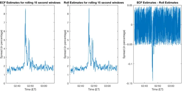
The results using log prices are presented in Figures 4 and 512and can be summarized as follows:
• Both estimators bsecf and bsRoll,1 produce almost identical (and roughly constant) results
throughout the sample period, except for the time from 2:45 p.m. to 2:49 p.m. ET,
dur-ing which the spread appears to spike, and then returns to its previous level. However, the increase is much more pronounced for bsRoll,1 than for our estimator bsecf. The turbulence in
12
market prices during this period, along with the simulation evidence in the previous section
on the robustness of bsecf in a heavy-tailed and asymmetric environment, suggest that bsRoll,1
might overstate the (increase in the) underlying liquidity cost, and thatbsecf provides a better approximation. This is consistent with the fact that both methods produce nearly identical results outside the window of extreme turbulence.
• The detected spike in the spread is consistent with the following passages in the SEC-CFTC report: "HFTs, therefore, initially provided liquidity to the market. However, between 2:41 and 2:44 p.m., HFTs aggressively sold about 2,000 E-Mini contracts in order to reduce their
temporary long positions." The estimates seem to pick up this temporary liquidity evaporation,
although with some time lag.
• However, we do not find any detectable early warning signs of a pending crash in the spread estimates, which we will document below. This is in contrast to, e.g., Easley et al. (2012), who
find that the (appropriately measured) market order flow became increasingly imbalanced in the hour preceding the crash, and that this imbalance contributed to the withdrawal of many
Figure 1: Transaction prices for E-Mini S&P futures (with maturity in June 2010) from 6 p.m. May 5, 2010 to 4:15 p.m. May 6, 2010, ET. Left: The last trading price for each second; Right:
The sequence of all transaction prices throughout the day.
Figure 2: Transaction prices for E-Mini S&P futures (with maturity in June 2010) from May 12,
2010, 6 p.m. to May 13, 2010, 4:15 p.m. ET. Left: The last trading price for each second; Right:
Figure 3: Transaction prices (left) and the number of trades in the last 30 seconds (right) for the
period of the Flash Crash.
Figure 4: Spread estimates in percentage terms, for rolling 30 second windows (i.e., last 30 seconds
Figure 5: Spread estimates in percentage terms, for rolling 15 second windows (i.e., last 15 seconds of transactions are used for estimation) during the period of the Flash Crash.
6.2.1 Forecasting the Flash Crash
We estimate a bivariate VAR model for(∆p,logs)using the 107 observations of spreads (computed
from non-overlapping thirty-second prior intervals) and the contemporaneous (log) prices. The results are presented in Table A1 of the online supplement (with standard errors in parentheses).
There is significant linear predictability in both series, although the spreads appear to be more predictable than returns according to the in-sample adjusted R-square measure.
The impulse response functions are shown in Figure A6 of the online supplement. They show that the return series is not significantly affected by shocks to the spread, whereas the spread does
respond negatively to return shocks. The spread series is positively autocorrelated with a significant response (persistence) to past shocks.
The variance decompositions indicate that return variation is almost exclusively due to past
returns, whereas spread variation is affected by past price especially after four lags. Despite this evidence of linear predictability in the two series over the whole period, linear models are not able,
by the residual graphs in Figure A7 of the online supplement.
6.2.2 Estimating the c.f. of the Fundamental Price Innovations εt
We have emphasized the estimation of the bid-ask spread parameters0, but it may also be of interest
to estimate features of the distribution of the innovation process. We could obtain estimates of the c.f. of the innovation process directly from the data:
b ϕε(u) :=
ϕT,2(u, u)
ϕT ,1(u)
, on V. (46)
For an illustration, we estimate the c.f. ϕε for three different points in time: before, at, and after the spike in the estimated spread (see Figures 4 and 5). Specifically, we choose the times 2:36 p.m., 2:46 p.m., and 2:56 p.m. ET, respectively. As in the previous section, we use all transaction prices
for the last 30 seconds in the estimation. We find the following, with the estimates displayed in Figure 6:
• For 2:36 p.m., we obtain an estimate that resembles the c.f. of a point mass at zero (i.e., the real part is almost always equal to 1 and the imaginary part is very close to zero), which is
intuitive. The data show that, during the tranquil periods of trading, the executed transaction price jumps up or down (with roughly equal probability) by at most a tick, which corresponds
to εt ≈ 0, i.e., there are no fundamental news, and the only price movements come from randomly arriving buy/sell orders.
• However, during the turbulent period, when the spread peaks at around 2:46 p.m., we obtain a significantly different behaviour of the latent price innovations. The estimate of Re(ϕε(u)) declines in a nearly linear fashion, which corresponds to the c.f. of a heavy-tailed distribution,
while the estimate of Im(ϕε(u)) appears to be nonzero, which corresponds to the c.f. of an asymmetric distribution. This, again, is in line with economic intuition, since the crash
in prices can be interpreted as reflection of a fundamental shock, represented by large and asymmetric innovations εt. In addition, this estimate supports our conjecture in Section 6.1 about the higher accuracy of our estimatebsecf compared to Roll’s estimatebsRoll,1 during the
turbulent period. Because based on the simulation evidence, the Roll’s estimator performs
worse under heavy-tailed and asymmetric innovations.
• After the peak turbulence, at 2:56 p.m., the estimate of the c.f. reflects a thin-tailed and symmetric regime again, close to the estimate that we obtain for 2:36 p.m..
Figure 6: Estimates of the c.f. ϕεof the latent price innovationsεtduring the Flash Crash of May 6, 2010. The plots/times refer to estimates before, at, and after the spike in the estimated spread,
as displayed in Figures 4 and 5.
6.2.3 Detecting Order Flow Imbalances
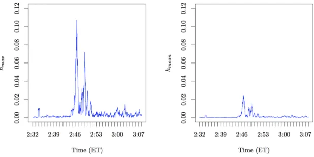
Eq.(36) shows the following : under a balanced order flow (i.e., It = ±1 with equal probability), the population quantityH(u, u0)is real-valued, while under order flow imbalance (i.e.,Pr(It= 1)6= Pr(It =−1)), the quantity H(u, u0) is complex-valued when u 6= u0. This yields a way to detect order flow imbalances by measuring the imaginary part of the empirical quantity HT(u, u0). In Figure 7, we plot the evolution of the two quantities
hmax := max (u,u0)∈U Im(HT(u, u0)) and hmean:= 1 |U | X (u,u0)∈U Im(HT(u, u0)) , (47)
during the period of the Flash Crash. Clearly, the two measures hmax and hmean spike during the peak turbulence (and are almost perfectly synchronized with the spread increase we detect). This indicates that not only the liquidity cost (as measured by the bid-ask spread) increases sharply, but
also the order flow becomes highly imbalanced during this period. This is in line with the economic intuition of a panic sale interpretation of the crash.
Figure 7: Indications of order flow imbalances during the Flash Crash of May 6, 2010. The
definitions of the quantitieshmax and hmean are given in Eq.(47).
6.2.4 Aggregation Robustness
In Section A3 of the online supplement, we show that our estimators are aggregation robust. For the basic Roll (1984) model, we estimate the spread at each second, using the non-overlapping returns
for every 2 (k= 2) and 5 (k= 5) transactions over the last 30 seconds. The results are presented in Figure A8 - A11 of the online supplement.
6.2.5 Adverse Selection Estimators
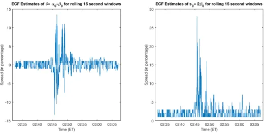
In Section 3, we consider the presence of an adverse selection component in the spread :
whereβ0 =s0/2 and α0 =s0/2 +δ. Using all trades over the last 15 and 30 seconds, we estimate
s= 2β andδ=α−β at each second. Estimation results using log prices are presented in Figures 8 and 913. The results show that in the run up to the Flash Crash, the adverse selection component of the spread was quite small. However, this rose substantially during the peak period.
Figure 8: The adverse selection case : spread estimates in percentage terms, for rolling 30 second
windows during the period of the Flash Crash.
Figure 9: The adverse selection case : spread estimates in percentage terms, for rolling 15 second
windows during the period of the Flash Crash.
7
Conclusions
In this paper we provide simple semiparametric estimators of the spread using transaction price data alone. We compare our method theoretically and numerically with the Roll (1984) estimator as well
as with the Hasbrouck (2004) estimator. Our estimators perform similarly to theirs when the latent
fundamental return distribution is Gaussian, but much better than theirs when the distribution is far from Gaussian, such as for heavy-tailed or asymmetric data.
Our c.f. based estimators are applied to the E-mini futures contract on the S&P 500 during the Flash Crash of 2010. We find that, during relatively tranquil times our estimator sbecf and the Roll estimator bsRoll,1 are very similar, while during the peak period of the Flash Crash, i.e.,
from 2:45 p.m. to 2:49 p.m. ET, the spread appears to spike, and then returns to its previous
level, but the increase is much more pronounced for the Roll estimator than for our estimator. The estimated c.f. of εt indicates that the fundamental innovation becomes much more heavy-tailed and asymmetric during the turbulent period. Along with the simulation evidence on the robustness
of our estimator bsecf in a heavy-tailed and asymmetric environment, it suggests that sbRoll might
overstate the underlying liquidity cost, and that bsecf provides a better approximation. This is consistent with the fact that both methods produce nearly identical results outside the window of extreme turbulence. We also find that the order flow becomes badly unbalanced and the adverse
selection component of the spread fluctuates substantially during the peak period of the Flash Crash. Both of these findings corroborate the work presented in the SEC/CFTC report on the days events
Acknowledgements
The authors would like to thank the guest coeditors, the two anonymous referees, Joel Hasbrouck, J. Huston McCulloch, and other seminar participants at Melbourne, NYU, Boston University,
Lan-caster, 2016 FERM and 2016 Shandong Econometrics Conference. Chen thanks Cowles Foundation
for research support. Yi acknowledges supports from National Natural Science Foundation of China (Grant 71471107 and 71501120). Yi is also affiliated with the Key Laboratory of Mathematical