Do Professional Traders Exhibit Myopic Loss
Aversion? An Experimental Analysis
MICHAEL S. HAIGH and JOHN A. LIST∗
ABSTRACT
Two behavioral concepts, loss aversion and mental accounting, have been combined to provide a theoretical explanation of the equity premium puzzle. Recent experimental evidence supports the theory, as students’ behavior has been found to be consistent with myopic loss aversion (MLA). Yet, much like certain anomalies in the realm of riskless decision-making, these behavioral tendencies may be attenuated among pro-fessionals. Using traders recruited from the CBOT, we do indeed find behavioral dif-ferences between professionals and students, but rather than discovering that the anomaly is muted, we find that traders exhibit behavior consistent with MLA to a
greaterextent than students.
ONE MAINSTAY AMONG ECONOMISTS IStheir fascination with anomalies and unsolved
puzzles. Arguably one of the most provocative enigmas in recent years is the eq-uity premium puzzle: Given the return of stocks and bonds over the last century, an unreasonably high level of risk aversion would be necessary to explain why investors are willing to hold bonds at all (Mehra and Prescott (1985)). Recently, Benartzi and Thaler (1995) combined two behavioral concepts—loss aversion (Kahneman and Tversky (1979)) and mental accounting (Thaler (1985))—to provide a theoretical foundation for the observed equity premium puzzle. While only a few experimental studies have tested Benartzi and Thaler’s myopic loss aversion (MLA) theory, the results thus far have been quite promising, as Thaler et al. (1997), Gneezy and Potters (1997), and Gneezy, Kapteyn, and Potters (2003) have all observed individual behavior consistent with the MLA conjecture.
∗Haigh is from the Office of the Chief Economist at the U.S. Commodity Futures Trading Commission and AREC, University of Maryland. List is from AREC and the Department of Economics, University of Maryland, and the NBER. Please direct correspondence to List at [email protected]. We wish to thank the journal editor, Richard Green, for his patience, perse-verance, and comments on earlier versions of the manuscript. An anonymous reviewer and Daniel Millimet provided very helpful comments. Liesl Koch helped prepare the manuscript and Jonathan Alevy provided able research assistance. Thanks also to John Di Clemente, former Managing Director of Research at the Chicago Board of Trade for authorizing the study. CBOT officials Dorothy Ackerman Anderson, Keith Schap, and Frederick Sturm also provided incredible support on site. Thanks to the University of Maryland for funding this research. The authors are grateful to Jana Hranaiova, seminar participants at the Washington Area Finance Association, and the Eastern Finance Association for their helpful comments. The views expressed in this paper are those of the authors and do not, in any way, ref lect the views or opinions of the U.S. Commodity Futures Trading Commission.
Yet, in light of some recent studies (e.g., List (2002, 2003, 2004)) that re-port market anomalies in the realm of riskless decision-making are attenuated among real economic players who have intense market experience, the current lot of experimental studies and their support of MLA may be viewed with cau-tion.1This point is strengthened given that there are numerous reasons to sus-pect that financial professionals’ behavior may differ from nonprofessional be-havior due to training, regulation, etc. (Burns (1985), Holt and Villamil (1986)). Locke and Mann (2000) take the argument a step further by suggesting that any research that ignores the use of professional traders is likely to be received passively because “ordinary” individuals are unlikely to have any substantial impact on market price since they are too far removed from the price discovery process.2
As a whole, these arguments suggest that behaviormaychange significantly when real market players are put to the task. To explore this issue within the realm of MLA, we make use of undergraduate students as our experimen-tal control group, and recruit 54 professional futures and options pit traders from the Chicago Board of Trade to examine if behavioral discrepancies exist across subject pools. Using an experimental protocol that is consistent with the extant literature, we find that professionals do indeed behave differently from undergraduate students. Yet, instead of displaying behavior inconsistent with the MLA conjecture, as we had expected, the professional traders exhib-ited behavior consistent with MLA to a greater extent than undergraduate students.
These findings, which support evidence from laboratory experiments using student subjects, may have important asset pricing and modeling implications. As the literature notes, the presence of MLA suggests that market prices of risky assets might be significantly higher if feedback frequency and decision f lexibility are reduced. In this sense, institutions may have the ability to inf lu-ence asset prices through changes in their information provisioning policies. As outlined in Gneezy et al. (2003, p. 821), this behavioral phenomenon appears to be what compelled Israel’s largest mutual fund manager, Bank Hapoalim, to change its information release about fund performance from every month to every 3 months, noting that “investors should not be scared by the occasional drop in prices.”
The remainder of our study proceeds as follows. In the next section, we provide a brief background of MLA and describe our experimental design. In Section II we report our results. Section III summarizes and concludes the paper.
1Indeed, Christensen-Szalanski and Beach (1984) make an even stronger argument noting that
the experimental literature using students is biased (see also Bonner and Pennington (1991)). Their main contention is that experimental findings of major anomalies have largely used student subjects, whereas those few studies that have employed professionals have usually reported perfor-mance more in line with mainstream theory. This line of argument is also an assumption implicit in other experimental research (e.g., Frederick and Libby (1986)).
2If one is interested in market behavior, it is important to recognize that it is behavior at the
I. Background and Experimental Design
Before becoming immersed in the experimental design, it is important to highlight what MLA is and why it is important to understand. As aforementioned, MLA is a behavioral theory that combines loss aversion and mental accounting. An agent is said to be loss averse if he is more acutely aware of losses than gains of equal size. More formally, loss aversion is the result of individuals having a “value function” defined with respect to the status quo. This value function is positive and concave over gains and is negative, convex, and more steeply sloped over losses (Kahneman and Tversky (1979)). Mental accounting refers to how individuals aggregate choices (explicitly or implicitly). In particular it refers to how transactions are evaluated over time (how often portfolios are evaluated) and cross-sectionally (whether they are evaluated as portfolios or individually). Mental accounting determines both the outcomes of decisions as well as the framing of those decisions. An agent who frames his decisions narrowly will tend to make shorter-term choices and an agent who frames outcomes narrowly will evaluate her losses and gains more frequently (Thaler et al. (1997)).
If agents evaluate their investments at high frequencies, there may be peri-ods of time where the return on a risky asset (i.e., stocks) is lower than those on a safe asset (i.e., bonds), whereas less frequent evaluation might suggest the opposite. Since losses are weighed more heavily than gains, the high-frequency evaluation will lead to greater dissatisfaction. If the agent considers perfor-mance over longer time periods, the riskier asset is likely to outperform the safer asset, and hence agents will place a higher value on stocks relative to bonds. An individual is, therefore, myopically loss averse if he evaluates gains and losses separately as soon as the information is consumed, rather than pool-ing the returns into a lifetime portfolio.
As an example of how MLA inf luences individual decision-making, assume that an agent is loss averse and weighs losses relative to gains at a rate of δ >1. Suppose also that the agent has a two-thirds probability of losing $1 and a one-third probability of winning $2.50. The expected utility of the gamble is thus 1/3(2.5)+δ2/3(−1), which takes on a positive value ifδ <1.25. If, on the other hand, the loss-averse agent evaluates three lotteries in combination, we may view her expected utility per decision task as follows: 1/27(7.5)+6/27(4)+ 12/27(0.5)+δ8/27(−3),δ2/3(−1), which is positive ifδ <1.56, effectively making the individual lottery sequence more attractive to a loss-averse individual than the aggregate lottery sequence.3
3To fully appreciate the effect of MLA on risk preferences, we consider an agent who must choose
between a stock with an expected return (and standard deviation) of 7% (20%) per year and a less volatile stock with a guaranteed 1% annual return. Using the assumptions above, we find that the appeal of the risky asset will be a function of the time horizon of the investor: An agent willing to wait longer before evaluating the outcome of the asset will find the stock more attractive than an equally loss-averse agent who evaluates sooner. Moreover, agents who differ in the frequency with which they evaluate outcomes will not derive the same utility from owning the stocks. To illustrate, consider the simple example in Thaler et al. (1997): Assume that the loss-averse utility takes the
Table I
Experimental Design
Subject Type Treatment F Treatment I
Students 32 32
Traders 27 27
Note:Numbers represent sample sizes. Treatment F had subjects placing bets in nine rounds; after each round, the subject was informed of the outcome. Treatment I was identical except subjects placed bets for three rounds at a time rather than for each round. Thus, subjects in Treatment F received frequent feedback, whereas subjects in Treatment I received infrequent feedback. A. Experimental Design
To study whether traders exhibit behavior consistent with the MLA conjec-ture, we used a straightforward 2×2 experimental design (see Table I). Be-cause one important goal of our research was to explore whether agents who are professional traders exhibited behavior in line with MLA, we used undergrad-uate students as our experimental control group. Using a between-person ex-perimental design, we included both undergraduate students and professional traders in two distinct treatments: Treatment F (denoting frequent feedback) and Treatment I (denoting infrequent feedback). And to ensure comparability with the extant literature, we followed Gneezy and Potters (1997) when crafting our experimental protocol and parameters.4In this spirit, our experimental de-sign should be considered an “artefactual field experiment” (see Harrison and List (2004)).
In Treatment F, subjects were confronted with a sequence of nine rounds in which they were endowed with 100 units per round (see below for exchange rate details). In each of the nine rounds, the subject decided what portion of this endowment (0, 100) she desired to bet in a lottery that returned two-and-a-half times the bet with one-third probability and nothing with two-thirds probabil-ity. As illustrated in the experimental instructions contained in Appendix A, subjects were made aware of the probabilities, payoffs, and the fact that the lottery would be played directly after all subjects had made their choices for that round. Thus, subjects played rounds one by one. Subjects were therefore aware of the fact that they could earn anywhere between 0 and 350 units in each round. Finally, subjects were informed that monies earned were to be summed and paid in private at the end of the experiment.
Contrasting with this “frequent feedback” environment is Treatment I, which is identical to Treatment F, except that in Treatment I agents placed their formU(w)=wforw≥0 andU(w)=2.5wforw<0 (wherewdenotes the change in wealth and 2.5 is the value of the agent’s loss aversion parameter). Under this scenario, the utility of investing in the stock would be−2.75: (1
2(27)+ 1
2 2.5(−13)) if evaluated myopically (one period) compared
to the utility of 1 for the bond. After two periods, however, the utility from owning the stock is 4.25: (1
4 2 (27)+ 1
2 (27−13)+ 1
4 5 (−13)), compared to the cumulative (noncompounded) return
from the bond of 2.
4Appendix A contains our experimental instructions for student Treatment F, which closely
follow Gneezy and Potters (1997). Instructions for Treatment I are similar to Treatment F, with the necessary adjustments.
bets in blocks of three. Rather than placing their round bet and realizing the round outcome before proceeding to the next round, in Treatment I agents decided in roundthow much of their 100-unit endowment they wished to bet in the lotteries for each of three rounds,t,t+1, andt+2. Following Gneezy and Potters (1997), we restricted the bets to be homogeneous across the three rounds. Most importantly, after subjects placed their bets, they were informed about the combined realization of the three rounds. This contrasts with our assignment of gains and losses after each round in Treatment F, and provides heterogeneity in the evaluation period.
Previous efforts have shown that this simple framing change can have re-markable effects on betting behavior. To cite just one example, using Dutch undergraduate students, Gneezy and Potters (1997) found that the average percent of endowment bet is significantly greater in the low feedback treat-ment compared to the high feedback treattreat-ment: 67.4% versus 50.5%.
As summarized in Table I, we recruited 64 subjects for our student treat-ments from the undergraduate student body at the University of Maryland. Each treatment was run in a large classroom on the College Park campus of the University of Maryland. To ensure that decisions remained anonymous, the subjects were seated far apart from each other. The trader subject pool included 54 professional traders from the CBOT.5Each of the trader treatments was run in a large room on-site at the CBOT. As in the case of the students, communi-cation between the subjects was prohibited and the traders were seated such that no subject could observe another individual’s decision (and payoffs).
Before moving to a discussion of the experimental results, we should men-tion a few noteworthy aspects of our experimental design. First, all treatments were run using pencil and paper. After subjects made their decisions and the lottery results were realized, experimenters circulated to ensure that individual payoffs were calculated correctly. Then, the agents made their decision for the next decision period. Second, whether a participant won or lost in any given round of the lottery depended on their personal win color. Participants won if their win color matched the round color that was drawn by the assistant, and lost if their win color did not match the round color. The outcome of the random events (the round color drawn) was announced publicly, and subjects were only aware of their own bets and whether they won or lost (i.e., they were not made aware of others’ round colors or bets). Third, in the student treatments, the exchange rate was 1:1 (1 cent for each unit), and in the trader treatments, the exchange rate was 4:1 (4 cents for each unit). Our decision to quadruple the stakes for traders was based on a detailed discussion with CBOT
5We refer to all subjects recruited from the CBOT as traders. However the 54 traders recruited
consisted of locals, brokers, clerks and exchange employees (e.g., f loor managers or market re-porters) who worked in the open outcry environment. We found no statistical difference between f loor participant types, hence we pool participants and collectively call them “traders.” This find-ing is intuitive since the average nonlocal/broker had accumulated approximately 9 year of f loor experience and many reported to have had several years of experience as either a local or bro-ker. Finally, the average trader (including nonlocals/brokers) was involved with about 537 traded contracts daily.
Figure 1. Comparing betting patterns.
officials about trader earnings.6 Fourth, data for the student (trader) treat-ments were gathered in four (four) distinct sessions and no subject participated in more than one treatment.
II. Results
Our key comparative static result is an examination of behavioral differences across frequent and infrequent treatments between subject types. To maintain consistency with the previous literature, we begin the empirical analysis by discussing findings from nonparametric statistical tests. We then extend these results by discussing empirical estimates from a panel data regression model. Since MLA predicts that the average bet in Treatment F should be less than the average bet in Treatment I, we directly compare betting levels in Figure 1, which places our data alongside the data reported in Gneezy and Potters (1997). Betting behavior summarized in Figure 1 is consistent with MLA. For in-stance, while traders bet on average nearly 75 units in Treatment I, they bet only 45 units in Treatment F. Our student data, which are consonant with the
6Our student exchange rate is very similar to Gneezy and Potters (1997) after adjusting for
exchange rate differences between the guilder and the U.S. dollar. CBOT officials suggested that designing a 30-minute game with an expected average payout of approximately $30.00 was more than a reasonable approximation to an average trader’s earnings for an equivalent amount of time on the f loor (in our experiment, the median trader’s earnings for 25 minutes was about $40.00). Indeed, postexperimental discussions with the traders indicated that these stakes were salient.
empirical findings presented in Gneezy and Potters (1997) and Thaler et al. (1997), exhibit a similar pattern: In Treatment I, students bet on average 62.50 units versus 50.89 units in Treatment F. Yet, the data indicate a curious pat-tern. While the University of Maryland undergraduate students exhibit behav-ior that is consistent with MLA, the effect is much less pronounced than the treatment effect observed among traders.
To assess these differences statistically and provide a sense of the temporal nature of the betting patterns, we average the amount bet at the individual level in rounds 1–3, 4–6, and 7–9 for Treatment F (to avoid data-dependency issues) and compare these data to observations in Treatment I. We present a summary of the raw data and statistical tests in the upper and lower panels of Appendix B. The upper panel of Appendix B can be read as follows: Row 1, column 1, at the intersection of “Rounds 1–3” and “Trader Treatment F,” denotes that the average trader in Treatment F bet 48.85 (with a standard deviation of 30.88) units in rounds 1–3. As a comparison, column 2 in this same row indicates that traders in those same rounds bet 66.22 in Treatment I. Using a nonparametric Mann–Whitney statistical test, we find that these bets are significantly different at the p < 0.05 level. This result is contained in the lower panel of Appendix B at the intersection of “Rounds 1–3” and “Trader Treatment F versus Treatment I” (z= −2.19;p=0.029).
Perusing the summary of empirical results in the lower panel of Appendix B reveals the strength of the treatment effect among dealers: In every block of three rounds, traders in Treatment I bet greater amounts than traders in Treatment F. Alternatively, we only find sporadic statistical significance among students.7This pattern of results also holds if we consider the average bet across all rounds (Rounds 1–9): Traders bet 74.29 units in Treatment I and 45.59 in Treatment F (a difference of 28.7) whereas students bet 62.50 in Treatment I and 50.89 in Treatment F (a difference of 11.61). Our raw data, therefore, provide a surprising insight: Professional traders exhibit behavior consistent with MLA to a greater extent than undergraduate students.
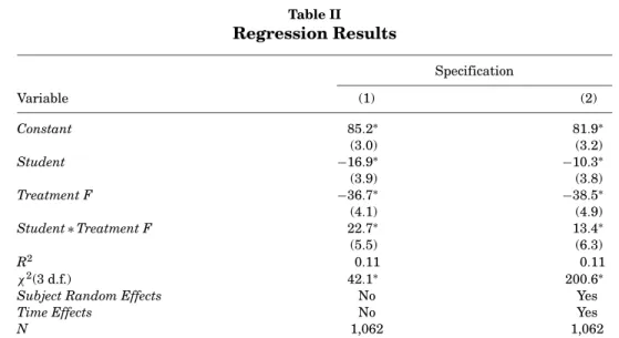
Although analysis of the raw data provides evidence to support this unex-pected finding, there has been little attempt to control for the panel nature of our data. To provide a robustness test, we estimate a panel data regression model in which we regressed the individual bet on a dummy variable for subject pool, a dummy variable for treatment, their interaction, and unobservable sub-ject and time effects. Because the subsub-ject pool and treatment dummy variables are static, we report panel data estimates from a random effects regression model (the rank condition would be violated if we estimated a fixed effects model).
Empirical results from two specifications are contained in Table II.8 Specifi-cation (1) is a simple Tobit regression model, while specifiSpecifi-cation (2) augments this baseline model by including subject and period random effects. Regardless
7Given the fact that subjects are confronted with an upper (100) and lower (0) bound, the
distribution must be non-normal. Moreover, results from the Kolmogorov–Smirnov test confirm the non-normality of the data.
8Note fromχ2tests presented in Table II that both of our models are significant at thep<0.01
Table II Regression Results Specification Variable (1) (2) Constant 85.2∗ 81.9∗ (3.0) (3.2) Student −16.9∗ −10.3∗ (3.9) (3.8) Treatment F −36.7∗ −38.5∗ (4.1) (4.9) Student∗Treatment F 22.7∗ 13.4∗ (5.5) (6.3) R2 0.11 0.11 χ2(3 d.f.) 42.1∗ 200.6∗
Subject Random Effects No Yes
Time Effects No Yes
N 1,062 1,062
Notes:Dependent variable is the individual bet. “Trader” is the omitted subject category and therefore represents the baseline group. Student (Treatment F) is the student (treatment) indicator variable that equals 1 if the subject was a student (in Treatment F), 0 otherwise.
Student∗Treatment F is the student indicator variable interacted with the frequent feedback treatment variable. Specification (1) is a Tobit model. Specification (2) is a random effects Tobit model. Theχ2values provide evidence of the models’ explanatory power. In both cases our model is
significant at thep<0.01 level. Standard errors are in parentheses beneath coefficient estimates. ∗Denotes significance at thep<0.05 level.
of which empirical assumptions one subscribes to, our estimation results sup-port the conclusions from the raw data. For example, in specification (2) we find that traders in Treatment F bet approximately 38.5 fewer units than traders in Treatment I, and this difference is significant at thep<0.01 level. The evidence is slightly weaker for students, where Treatment F subjects bet approximately 25 (13.4–38.5) fewer units than students in Treatment I, a noteworthy differ-ence, but one that is significantly less than the 38.5 unit difference observed between traders. This finding can be gleaned from the coefficient estimate of theStudent∗Treatment Finteraction term in Table II, which is significant at thep<0.05 level.9
III. Concluding Remarks
Two behavioral concepts, loss aversion and mental accounting, have recently been combined to provide a theoretical explanation of the equity premium puzzle (Benartzi and Thaler (1995)). Although only a few empirical tests have been carried out to explore the predictive power of the theory (e.g., Thaler et al. (1997), Gneezy and Potters (1997), Gneezy et al. (2003)), the experimental tests
9We also included a second part of the experiment whereby subjects bet using their own funds
earned from part 1. We exclude summary statistics of these data to conserve space, but note that the pattern of results for personal funds is consistent with the betting patterns observed above. See Appendix A for part 2 instructions.
to date have provided results consistent with the theory. Yet, inference from these experiments is open to criticism because it is based on observing the be-havior of undergraduate students. This can be problematic because observed treatment effects among students may not be representative of behavior in naturally occurring environments, where selection effects may have created distinct populations of economic decision-makers. Combining this insight with the fact that some recent field studies (e.g., List (2002, 2003, 2004) indicate that market experience attenuates certain market anomalies in riskless settings, we suspect that the current evidence supporting MLA may be viewed with caution. To provide initial insight into the robustness of the extant literature, we re-cruited futures and options traders to participate in an experiment. Making use of undergraduate students as our control group, we find an unexpected result: While the data suggest that both traders and students exhibit investment be-havior in line with MLA, traders exhibit this bebe-havior to agreaterextent than students. At a fundamental level, this result is important, since our traders, who are vital components of the price discovery process, exhibit more evidence of this type of behavior thananyother subject pool that has been evaluated to date.
A few normative and positive implications naturally follow. First, our findings suggest that expected utility theory may not model professional traders’ behav-ior well, and this finding lends credence to behavbehav-ioral economics and finance models, which are beginning to relax inherent assumptions used in standard financial economics. In a positive sense, these findings have direct implications on the communication strategies for fund managers, whereby revealing infor-mation on a less frequent basis means that the likelihood of incurring a loss is reduced. Moreover, providing less freedom to adjust (i.e., inducing agents to think in a more aggregated way) might reduce the likelihood that a sell-off en-sues after a minor setback. This intuition follows Gneezy et al. (2003), who note that if market information becomes more readily available at a lower cost one might expect it to be used more often—hence affecting behavior over riskier assets and therefore relative prices.
Appendix A: Experimental Instructions for Student Treatment F A.1. Instructions for Part 1
Part 1 of the experiment consists of nine successive rounds. In each round you will start with an amount of 100 units (1 unit=1 cent). You must decide which part of this amount (between 0 units and 100 units) you wish to bet in the following lottery:
You have a two-thirds chance (67%) to lose the amount you bet and a one-third chance (33%) to win two-and-a-half times the amount you bet. You are requested to record your choice on your registration form. Suppose you decide to bet an amount ofXunits (100≥X≥0) in the lottery. Then, you must fill in the amountXin the column headed Amount in lottery, in the row with the number of the present round.
Whether you win or lose in the lottery depends on your personalwin color. This color is indicated on top of your individual sheet. Your win color can be red, blue, or white, and is the same for all nine rounds. In any round, you win in the lottery if your win color matches theround colorthat will be drawn by the assistant, and you lose if your win color does not match the round color.
The round color is determined as follows. After you have recorded your bet in the lottery for the round, the assistant will, in a random manner, pick one color from a cup containing three colors: red, blue, and white. The color drawn is the round color for that round. If the round color matches your win color you win in the lottery; otherwise you lose. Since there are three colors, one of which matches your win color, the chance of winning in the lottery is one-third (33%) and the chance of losing is two-thirds (67%).
Hence, your earnings in the lottery are determined as follows. If you have decided to put an amount ofXunits in the lottery, then your earnings in the lottery for the round are equal to−Xif the round color does not match your win color (you lose the amount bet) and equal to+2.5Xif the round color matches your win color (you win two-and-a-half times the amount bet).
The round color will be shown to you by the assistant. You are requested to record this color in the columnRound colors, underwinorlose, depending on whether the round color does or does not match your win color. Also you are requested to record your earnings in the lottery in the columnEarnings in lottery. Your total earnings for the round are equal to 100 units (your starting amount) plus your earnings in the lottery. These earnings are recorded in the column Total earnings, in the row of the corresponding round. Each time we will come by to check your registration form for errors in calculation.
After that, you are requested to record your choice for the next round. Again you start with an amount of 100 units, a part of which you can bet in the lottery. The same procedure as described above determines your earnings for this round. It is noted that your private win color remains the same, but that for each round, a new round color is drawn by the assistant. All subsequent rounds will also proceed in the same manner. After the last round has been completed, your earnings in all rounds will be summed. This amount determines your total earnings for part 1 of the experiment. Then, the instructions for part 2 of the experiment will be announced.
A.2. Instructions for Part 2
Part 2 of the experiment is almost identical to part 1, but differs in two respects. First, part 2 consists of three rounds (instead of nine rounds). Second, in part 2 you do not get any additional starting amount from us. You play with the money that you have earned in part 1. To that purpose, we first divide your earnings in part 1 by three. The resulting amount is yourstarting amount S
for each of the three rounds. Again you are asked which part of this amount (between 0 andS) you wish to bet in the lottery.
You have a two-thirds chance (67%) of losing the amount you bet and a one-third chance (33%) of winning two-and-a-half times the amount you bet.
You are asked to record your choice on the registration form. If you decide to bet an amount ofXunits (S≥X≥0), then you must fill in the amountXunder
Amount in lottery.
Your privatewin coloris the same as in part 1 and can be found on top of your registration form. After you have recorded your bet for the present round, the assistant will again, in a random manner, pick one color from a cup containing three colors: red, blue, and white. The color drawn is the round color. If this round color matches your win color, you win in the lottery, otherwise you lose.
If you have decided to bet an amountXin the lottery, then your earnings in the lottery are equal to−X if the round color does not match your win color (you lose the amount bet for the round) and equal to+2.5Xif the round color does match your win color (you win two-and-a-half times the amount bet for the round).
You are again requested to record the round color and your earnings in the lottery on the registration form. Your total earnings for the round are equal to your starting amountSplus your earnings in the lottery. You are asked to record these on your registration form. We will come by to check your form for errors.
After that you are requested to make your choice for the next round. Again you can choose to bet part of your starting amount in the lottery. The same procedure as described above determines your earnings. Round 3 will proceed in the same manner. After that, your earnings in the three rounds will be added. This amount determines your total earnings in parts 1 and 2 of the experiment.
Appendix B
Raw Data Summary
Average Bet (SD)
Trader Trader Student Student
Treatment F Treatment I Treatment F Treatment I Rounds 1–3 48.85 (30.88) 66.22 (27.50) 42.77 (31.16) 56.50 (25.75) Rounds 4–6 39.10 (33.11) 75.56 (24.58) 51.77 (30.64) 62.72 (26.69) Rounds 7–9 48.83 (34.24) 81.41 (22.74) 58.13 (28.52) 68.28 (26.88) Rounds 1–9 45.59 (32.69) 74.29 (25.49) 50.89 (30.48) 62.50 (26.56)
Mann–Whitneyz-Statistics (p-Values)
Trader Student
Treatment F Versus Treatment I Treatment F Versus Treatment I Nonparametric Statistical Test Results
Rounds 1–3 −2.19 (0.029) −2.35 (0.019)
Rounds 4–6 −3.90 (0.000) −1.48 (0.138)
Rounds 7–9 −3.55 (0.000) −1.45 (0.146)
Rounds 1–9 −3.48 (0.000) −1.82 (0.069)
Notes: Columns 1–4 in the upper panel summarize trader and student betting behavior over rounds. Columns 1–4 in the lower panel summarize Mann–Whitney tests of the differences in behavior across treatment type.
REFERENCES
Becker, Gary S., 1962, Irrational behavior and economic theory,Journal of Political Economy70, 1–13.
Benartzi, Shlomo, and Richard Thaler, 1995, Myopic loss aversion and the equity premium puzzle,
Quarterly Journal of Economics110, 73–92.
Bonner, Sarah, and Nancy Pennington, 1991, Cognitive processes and knowledge as determinants of auditor experience,Journal of Accounting Literature10, 1–50.
Burns, Penny, 1985, Experience in decision making: A comparison of students and businessmen in a simulated progressive auction, in V. L. Smith, ed.Research in Experimental Economics(JAI Press, Greenwich).
Christensen-Szalanski, Jay J., and Lee Roy Beach, 1984, The citation bias: Fad and fashion in the judgment and decision literature,American Psychologist39, 75–78.
Frederick, David, and Robert Libby, 1986, Expertise and auditor’s judgments of conjunctive events,
Journal of Accounting Research24, 270–290.
Gneezy, Uri, Arie Kapteyn, and Jan Potters, 2003, Evaluation periods and asset prices in a market experiment,Journal of Finance58, 821–838.
Gneezy, Uri, and Jan Potters, 1997, An experiment on risk taking and evaluation periods,Quarterly Journal of Economics112, 631–645.
Harrison, Glenn W., and John A. List, 2004,Field Experiments42, 1013–1059.
Holt, Charles A., and Anne Villamil, 1986, The use of laboratory experiments in economics: An introductory survey, in S. Moriarity, ed.Laboratory Market Research(University of Oklahoma Press, Norman, OK).
Kahneman, Daniel, and Amos Tversky, 1979, Prospect theory: An analysis of decision under risk,
Econometrica47, 263–91.
List, John A., 2002, Preference reversals of a different kind: The more is less phenomenon,American Economic Review92, 1636–1643.
List, John A., 2003, Does market experience eliminate market anomalies?Quarterly Journal of Economics118, 41–71.
List, John A., 2004, Neoclassical theory versus prospect theory: Evidence from the marketplace,
Econometrica72, 615–625.
Locke, Peter R., and Steven Mann, 2004, Professional trader discipline and trade disposition. Jour-nal of Financial Economics(forthcoming).
Mehra, Rajnish, and Edward Prescott, 1985, The equity premium: A puzzle,Journal of Monetary Economics15, 145–161.
Thaler, Richard H., 1985, Mental accounting and consumer choice,Marketing Science4, 199–214. Thaler, Richard H., Amos Tversky, Daniel Kahneman, and Alan Schwartz, 1997, The effect of myopia and loss aversion on risk taking: An experimental test,Quarterly Journal of Economics