Using context for the combination of off-line and on-line learning

Using context for the

combination of off-line and

on-line learning

Jeffrey F. Queißer

Intelligent Systems - Faculty of Technology University of Bielefeld

A thesis submitted for the degree of Master of Science (M.Sc.)

Abstract

This thesis proposes a classifier combination system in the context of travers-ability classification. The goal is to enable a system to utilize on-line train-ing for a fast adaptation to new and changtrain-ing environments. Moreover the on-line classifier is able to handle additional context information that is only available in the on-line environment. Therefore the learning system is based on two different classifiers: One off-line trained classifier is trained in a pre-processing step and one on-line classifier that adapts its internal rep-resentation according to the current task complexity. The off-line classifier allows to use general information that is available for the target application area and can be trained by a slow exhaustive off-line training process. The on-line classifier is accountable for a specialization during operation, there-fore it is desirable to achieve fast and efficient learning due to the high costs of the acquisition of labeled training data. To achieve a system that is able to combine different types of classifiers that use different and dynamic input spaces an external probability estimation technique is used. The experi-mental results highlight the benefits of the proposed classifier combination system in comparison to a solution that is based on a single classifier. It was shown that the classifier combination leads to a fast system adaptation to a new environment that was used for on-line learning. Moreover a spe-cialization of the classifiers in a divide-and-conquer manner to certain data set sub-spaces can be observed. The comparison between systems that used different combinations of input features shows that additional context in-formation in combination with a feature weighting technique can be able to improve the system performance. The introduction of a probability thresh-old for sample rejection allows a considerably performance increase of the classified samples.

Acknowledgements

I would like to express my appreciation to the Honda Research Institute Europe and my supervisors: Dr. Heiko Wersing and Dr. Britta Wrede. Thanks for giving me the opportunity to be part of the HRI-EU for the research involved with this master thesis. Special thanks to the former HRI-EU employee Dr. Stephan Kirstein for his efforts to make this master thesis possible and Dr. Mathias Franzius for his support in relation to python and the utilized simulation environment. Moreover I want to say thank you to all other employees of the HRI-EU for fruitful discussions and a positive working atmosphere.

Contents

1.3 Plan of the Manuscript . . . 4

2 Related Work 5 2.1 Context . . . 7 2.1.1 Feature Weighting . . . 8 2.2 Classifier Combination . . . 12 2.3 Traversability Classification . . . 14 3 Learning Method 17 3.1 Learning Architecture . . . 17 3.1.1 Realization . . . 20 3.2 GRLVQ and GMLVQ Learning . . . 22 3.3 iGMLVQ Extension . . . 24 4 System 25 4.1 Simulator . . . 26 4.2 Data Sets . . . 27 4.3 Test Framework . . . 27 4.3.1 Data iterator . . . 27 4.3.2 Performance analysis . . . 27

4.3.3 Ground truth . . . 27 4.3.4 Control logic . . . 28 4.3.4.1 Image patcher . . . 28 4.3.4.2 Feature extraction . . . 28 4.3.4.3 Context utilization . . . 28 4.3.4.4 Off-line classifier . . . 28 4.3.4.5 On-line classifier . . . 29 4.3.4.6 Reliability matrix . . . 29 4.3.4.7 Decision module . . . 29

5 Abstract Data Set 31 5.1 Artificial Data Set I . . . 31

5.2 Artificial Data Set II . . . 36

5.3 Conclusion . . . 40

6 Simulator Based Data Sets 41 6.1 Simulation Environment . . . 41 6.2 Scenario Environment . . . 42 6.2.1 Data sets . . . 44 6.3 Feature Extraction . . . 45 6.4 Classifier Combination . . . 47 6.4.1 Parameter optimization . . . 49 6.4.2 Contextualization . . . 51

6.4.3 Comparison to solely on-line training . . . 55

6.4.4 Visualization of classification results . . . 56

6.4.5 Prototype visualization . . . 60

6.4.6 More complex data set and additional features . . . 62

6.4.7 Rejection rate . . . 66

6.5 Conclusion . . . 67

7 Discussion 69 7.1 Further Work . . . 71

CONTENTS

List of Figures

2.1 Wrapper method concept . . . 10

3.1 Probability estimation . . . 17

3.2 Working principle of the used learning system . . . 19

4.1 Software architecture . . . 25

5.1 Artificial data set I visualization XY . . . 32

5.2 Artificial data set I visualization XZ . . . 33

5.3 Distribution of nodes after training using data set I . . . 33

5.4 System evaluation during training with artificial data set I . . . 35

5.5 Artificial data set II visualization . . . 36

5.6 Single run system evaluation . . . 37

5.7 System evaluation during training with artificial data set II . . . 38

5.8 Prototype representation of the artificial data set . . . 39

6.1 Environment I . . . 43

6.2 Environment II . . . 44

6.3 Feature reconstruction error . . . 45

6.4 Reconstruction visualization . . . 46

6.5 System performance . . . 47

6.6 Combination gain during training process . . . 48

6.7 Node insertion threshold sensitivity . . . 50

6.8 Probability history . . . 51

6.9 Λ matrix visualization . . . 55

6.11 Visualization of the classification result: View 160 & view 2980 . . . 58

6.12 Visualization of the classification result: View 1040 & view 20 . . . 59

6.13 Explanation of classifier visualization . . . 60

6.14 Node visualization of the on-line classifier . . . 61

6.15 Simulation environment using time information . . . 65

6.16 Distribution of the estimated probability . . . 66

List of Tables

2.1 Overview of different classifier combination methods. . . 13

6.1 System evaluation using context information . . . 52

6.2 Detailed system evaluation on confusable objects . . . 53

6.3 Detailed system evaluation on non confusable objects . . . 53

6.4 GMLVQ Λ-matrix used for distance estimation . . . 55

6.5 System Evaluation using context information and time simulation . . . 63

6.6 Detailed system evaluation on confusable objects . . . 64

6.7 Detailed system evaluation on non confusable objects . . . 64

A.1 Database visualization of the simulated environment used for off-line learning. . . 74

A.2 Database visualization of the simulated environment used for on-line learning. . . 75

A.3 Database visualization of the simulated environment used for on-line learning including additional time simulation. . . 76

1

Introduction

Regardless of the fact that computer vision made huge progress in the past fifty years, current methods and architectures are far away from the performance and robustness of what the human brain is capable to achieve. The Scale-invariant feature transforma-tion (SIFT) introduced by Lowe [1], is one of the newer, powerful and commonly used techniques to realize invariant object recognition that can deal with clutter and partial occlusion. The extracted feature descriptors are robust to different image scales, noise, illumination and geometric distortion. Nevertheless robust features are not sufficient to build a flexible and universal object recognition system. Generalization, categorization, multimodality or life-long learning for example are quite difficult to handle and require strategies with higher cognitive abilities to get solved. Most artificial learning systems completely rely on labeled training data in comparison to animals and humans that can extract meaningful representations from unlabeled data. To overcome this limita-tion the learning with solely or unlabeled data is beneficial since generalimita-tion of labeled training data is typically expensive. The combination of using labeled and unlabeled data is commonly termed semi-supervised learning. The basic concept is to enable a system to improve its internal representation based on a large amount of unlabeled data. Thereby semi-supervised learning combines the advantage of a higher reachable performance with less labeled training samples. The usage of only unlabeled data is referred to unsupervised learning.

An interactive on-line learning scenario for example requires an adaptation of the in-ternal representation coupled with a short training time. A human tutor should not have to provide a large amount of supervised training examples. Rather the learning

system itself should use just a small amount of meaningful examples given by a human tutor to get a coarse understanding of the data distribution and a much lager amount of unlabeled data samples to refine the borders and distributions of the represented data.

Unfortunately data samples that can only be labeled unreliably by a certain system improve the representation of the used classifier most, because these samples are com-monly not well represented in the network. In comparison to this, data samples that are easy to label are normally already well represented by the current state of the network. This is a strong disadvantage of architectures that utilize self-classification, a technique that forces a classifier to generate its own training data.

In the field of autonomous robots there exists another option for the generation of labeled training data. The exploration of the environment can lead, by trial and error, to labeled training data for the performed actions. But one has to mention that in the majority of cases environment exploration is a slow process that can not provide sufficient amount of training samples. Therefore an autonomous on-line system relies on a learning system that is able to provide good learning results using only a small training set.

This work exploits the capabilities of a learning system that is designed to be used in an unsupervised autonomous robot that has to solve the problem of traversability classification. The proposed learning method is not able to handle unlabeled training data, moreover the estimation of labels is motivated by an exploration phase of the autonomous system. The learning system approach that is discussed here targets the problems of classifier combination and the utilization of additional knowledge. Fur-thermore the system should be capable of on-line and incremental learning. Therefore the system uses two competing classifiers. One classifier is trained by an pre-processing step and represents the initial configuration of the system. The second classifier is able to handle on-line learning and adapts its model to the current problem complexity. The off-line training process is able to insert general knowledge in a well-trained classifier using many training samples. The on-line training process incorporates the ability of on-line adaptation to new environments with regarding the face that the usage of la-beled training samples is expensive. Additional context information that is beneficial for the learning task is only available during on-line learning.

1.1 Scenario

1.1

Scenario

The scenario used for this thesis uses two different environments. The first environment is available during the factory configuration of the learning system and is used to build up the representation of the off-line classifier. The second environment represents the local conditions that can be found in the application area. This environment is used for on-line training. Since the configuration, that can be done in a pre-processing step, is not able to cover all variability that is present in the application area, the data set used for off-line training has less structural complexity than the data set used for on-line training. Moreover additional context information like position, rotation or time information is only available for the on-line environment. The scenarios cover an outdoor area including different non traversable objects like trees, buildings and other obstacles. The traversable ground has a high texture variability that includes flowers and sandy spots. The on-line classifier introduces a third class of ignorable objects, these are objects that do not represent the ground but are traversable like leaves or a wooden veranda. The scenarios are designed in a way that objects that have a similar visual appearance do not always have the same class affiliation, like a wooden wheelbarrow and a wooden veranda or a heap of leaves and leaves that are arranged underneath a tree. This ambiguous environment design raises the importance of using additional context information to be able to solve the classification task.

1.2

Aims

The aim of this thesis is to explore the capabilities of a classifier combination system that is capable of on-line learning. The system should be able to utilize additional feature dimensions. This context information is only available to the on-line classifier, because it is not useful for the off-line environment. Therefore the classifiers have different input spaces. The resulting system should be evaluated by the use of data sets generated in a simulation environment. This artificial environment should model a typical outdoor scenario.

These aims lead to the following tasks that have to be accomplished: • Adapt and utilize 3D simulator

• Plan and implement experimental framework • Realize an abstract data simulation

• Implement the proposed classifier algorithm • Train off-line classifier

• Train and evaluate classification system

1.3

Plan of the Manuscript

The second chapter 2 mentions related work that was done in the field of machine learning, categorization, semi-supervised and unsupervised learning techniques, con-textualization, feature weighting and selection, classifier combination techniques and traversability classification. The following chapter 3 presents the learning method used in this thesis and the used classifiers in detail. The subsequent chapter 4 introduces the software system used for data set generation and the experimental setup of the pro-posed learning system. The following chapter 5 shows the results of the experiments that use artificial data set configurations. Experiments using data from the simulated environment can be seen in the chapter 6. This chapter shows a much more detailed evaluation of the learning system and presents in addition different visualizations of resulting state of the learning system. Thereafter the conclusion in chapter 7 gives an overview of the achieved goals and hints for further work that could be done regarding this system.

2

Related Work

There are several powerful learning methods available, but according to the state of the art only a few of them are capable of dealing with incremental and on-line learning. A crucial capability of incremental learning refers to the ability of a network architecture to adapt its complexity to the intricacy of the current task. Most commonly used classifiers are the Multi-Layer Perceptron (MLP) proposed by Rumelhart et al. [2] and the Support-Vector Machine (SVM) presented by Boser et al. [3]. An MLP network is composed of one input layer, one output layer and a number of hidden layers. They can be seen as universal function approximators, but standard MLPs are not able to fulfill the requirements for incremental learning since the network structure must be predefined. Moreover all connections are changed at each training step. This results in a corruption of older representations if not all data samples are presented repetitively. A SVM defines hyper plane class borders to maximize the distances of those class borders to the given data samples. To handle even non-linear separable data, the feature space gets extended by different non-linear kernel functions, but similar to MLP it can not deal efficiently with incremental learning and a changing training ensemble as shown by Kirstein et al. [4].

Category Learning To face the challenge of visual category learning there were lots of different approaches utilized. For example generative probabilistic models, Mc-Callum & Nigam [5] successfully applied a semi-supervised EM based method on text classification, SVM or boosting by Viola & Jones [6]. Most of the used approaches are off-line batch-learning systems, which cannot deal with incremental- or on-line

learn-ing. To overcome this limitation, several incremental learning techniques have been proposed, like vector quantization that is one common class of learning methods.

Vector Quantization There exist various vector quantization techniques, since the prototype based representation has the benefit that incremental learning can be achieved quite easily without changing the whole representation. Due to the ability of an incre-mental node insertion into the network. One of the intensively used vector quantization approaches are Self-Organizing Maps (SOM) by Kohonen [7], which are artificial neural networks that reduce the dimensionality of data. Additionally they preserve the topo-logical properties of the input. A standard SOM has a predefined node structure and is not capable of dealing with incremental learning, moreover this type of network can not deal with supervised data and is therefore not applicable for a semi-supervised learning scenario. The Learning Vector Quantization (LVQ) by Kohonen [7] and Neural Gas (NG) by Martinez & Schulten [8] approaches represent the data by single prototypes, the LVQ has no constraints to preserve topological properties. On each training step the best matching prototype (LVQ) or a weighted set of best matching prototypes (NG) get shifted in the direction of the input vector. Prototype-based learning methods have the advantage that learning only affects a small portion of the overall network. This has a positive effect on incremental learning and network stability. LVQ includes a class assignment of each prototype so that supervised learning is possible. Furthermore there exist related methods like the Growing Neural Gas (GNG) by Fritzke [9] that overcome the limitation of a predefined network structure by adding further nodes from time to time. The variant incremental learning vector quantization (iLVQ), as introduced by Kirstein et al. [10] is an enhanced LVQ based approach. There each node has a specific learning rate that guarantees the stability of acquired knowledge. Due to the addition of nodes to the network, incremental learning is possible as well.

Unsupervised and Semi-Supervised Learning Common unsupervised learning methods are clustering algorithms and Self-Organizing Maps by Kohonen [7]. One way to achieve semi-supervised learning are generative models like Gaussian mix-ture models as shown by McCallum & Nigam [5]. This method assumes a model p(x, y) = p(y)p(x|y). Where p(x|y) covers a Gaussian mixture model, therefore the data distribution is approximated by a set of cluster centers and covariance matrices.

2.1 Context

One labeled data sample could then label all other data samples inside the same clus-ter. This assumes that the model assumption is correct. If this is not the case it could reduce the resulting performance (as shown by Cozman et al. [11]). The mixture com-ponents are in practice identified by the Expectation Maximization (EM) algorithm by Dempster et al. [12]. It has the disadvantage that it is likely to converge to a local maximum. This can result in wrong classified unlabeled data that has a negative affect to the confidence of the learning system. Further methods are for example graph-based semi-supervised approaches, where each node represents a labeled or an unlabeled data sample and the edges with optional weights reflect the similarity of those samples. The next step is to estimate a functionf that fulfills two constraints, first it should give a good approximation of the graph and second it should be smooth on the whole graph. This can be achieved by optimizing the difference between the approximation of the real graph in combination with regularization to prevent over-fitting. The problem of graph-based methods are, that they strongly depend on the graph structure and the assigned edge weights. There are several methods that deal with the optimization problem of graph-based methods, an expatiate on this and the previous methods can be found in the survey by Zhu [13]. To achieve incremental and on-line learning of categories Kirstein et al. [14] presented a framework that autonomously bootstraps the visual representation. The learning process is divided into two phases, first a super-vised training and after this the unlabeled training data gets classified by the internal representation without the need of the original training set.

2.1

Context

With the increasing complexity of tasks that are addressed by cognitive systems, infor-mation about the context in which the system operates can lead to a better performance. As mentioned by Calisi et al. [15] different robotic tasks ranging from robot behavior to perception can benefit by this contextualization. Calisi proposes a classification scheme that divides context into several layers of abstraction:

• Environmental Context • Process Context

The mentioned Environmental Context represents a high level information which repre-sents the abstract structure of the environment like rooms and corridors. The Process Context represents low-level information that can be used to improve the underlying mapping process in terms of speed and robustness. The source of information that can be used for contextualization is not restricted to a certain type. For example Hese & Schmullius [16] evaluated the use of context information for forest change classifica-tion. For this task the distance of deforested areas to linear object classes are used as additional information, because they can give a hint for human involved deforestation.

2.1.1 Feature Weighting

Removing irrelevant and redundant features can have positive consequences for the underling classifier. Since a reduced input space can eliminate unnecessary classifier complexity and therefore more cost-effective predictors can be realized, as shown by Guyon and Elisseeff [17]

As mentioned by Kirstein [18], feature selection methods can be divided into three types:

1. Filter Methods 2. Wrapper Methods 3. Embedded Methods

The filter methods are computationally less expensive than wrapper methods and ro-bust against over-fitting, whereas wrapper methods tend to find better solutions for feature subset selection. In comparison to the other methods, embedded methods have the drawback that they can only be used in a complete recognition architecture, but this integration avoids additional computation time and can lead to an improved interaction between the classifier and the feature selection process.

Filter Methods select the appropriate features with no regard to the classifier. They can be seen as a dimension reduction pre-processing step.

One basic filter method is the document frequency. This method uses an occurrence counting of each feature to generate a feature ranking. Then the most frequent or least frequent occurring features are then selected for classification. Other ranking methods

2.1 Context

like chi-squared test and Information gain can be also used, which are explained in Forman [19]. He did an extensive empirical study of different feature selection metrics. Another selection can be made on the base of the relevance of each feature. The Relief-Algorithm proposed by Kira & Rendell [20] determines reliability weightswiby the use

of the update rule:

wi=wi+ xi−nearmissi νi 2 − xi−nearhiti νi 2 (2.1) The termxi represents theith dimension of the current input sample,nearmissi is the

ith dimension of the closest sample vector with the another class label and nearhiti is

theith dimension of the closest sample vector with the same class. ν is a normalization factor. One feature of a set of m features is selected if the relevance exceeds a certain thresholdτ and the relevance is given by:

Relevance= 1

mW (2.2)

The determination of nearhit and nearmiss is based on the euclidean distance on the data space. Kira & Rendell [20] could show that the Relief-Algorithm employs only a few heuristics which has a positive effect on the robustness of feature selection. Moreover the algorithm is tolerant to noise and has a polynomial complexity. But it is not optimal in the sense that the subset of features that is selected by this algorithm is not always the smallest.

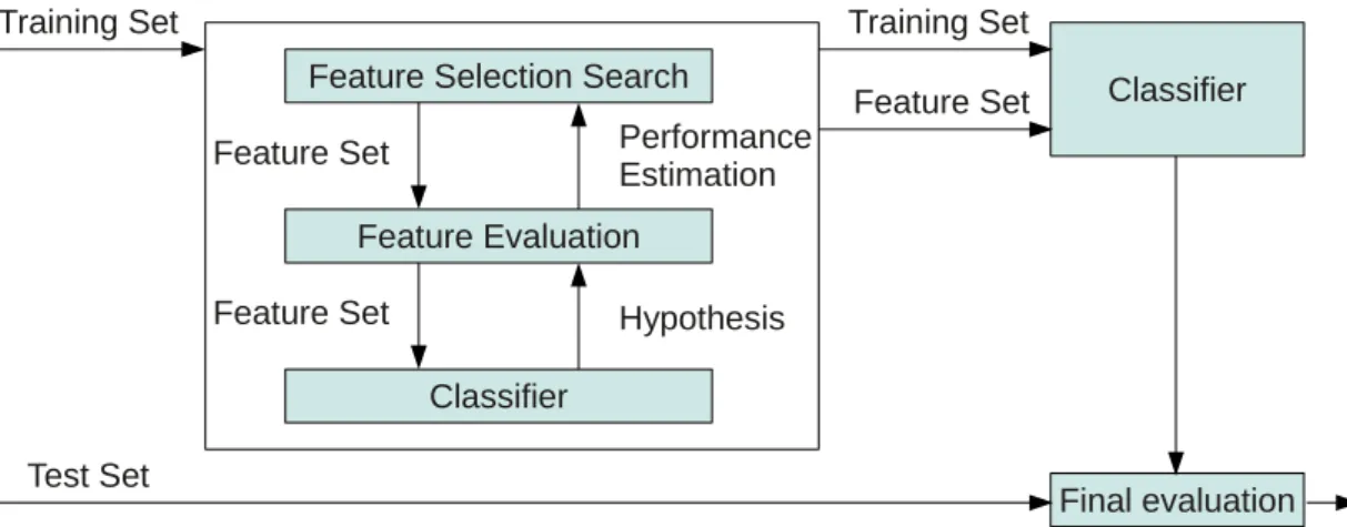
Wrapper Methods In comparison to Filter Methods, the Wrapper Methods utilize the classifier as a Black-Box. As mentioned by Kohavi & John [21] this supervised method has to focus its attention on those features that help to solve a given problem and ignore the other features. The filter Methods wrap around a Black-Box classifier as shown in fig. 2.1 The goal is to maximize the performance of a supervised classifier. The idea is to evaluate the classification accuracy using different feature subsets. Finally the feature subset with the highest classification accuracy is used as the final feature set.

One technique to realize a feature selection is Information Bottleneck as published by Tishby et al. [22]. This method is based on Mutual Information. The amount of

Feature Selection Search Feature Evaluation Classifier Feature Set Feature Set Performance Estimation Hypothesis Classifier Final evaluation Training Set Feature Set Training Set Test Set

Figure 2.1: Wrapper method concept - The wrapper method has no insights into the functionality of the used classifier. Therefore the classifier is used as a Black-Box. A feature selection tries to select those features that are able to improve the classification result. Adapted from Kohavi & John [21]

information stored by this technique about the data spaceY represented in the reduced feature space ˜X is given by:

IX˜;Y=X y∈Y X ˜ x∈_X˜ p(y,x˜)log p(y,x˜) p(y)p(˜x) ≤I(X;Y) (2.3)

Its obvious that the information of the reduced feature setIX˜;Y, as given in 2.3, can not exceed the information of the full feature setI(X;Y). The aim is now to conserve most information about the data space and to minimize the complexity of the feature space. This be interpreted as minimizing IX˜ :X, what leads to a minimization of the function: L[p(˜x|x)] =I ˜ X;X −βI ˜ X;Y (2.4) Another way to obtain a set of optimized features are genetic algorithms as mentioned by Mitchell [23]. A genetic algorithm defines a population of individuals and a fitness function that evaluates the fitness of the individuals. Each individual has a chromosome commonly represented as a binary vector. This chromosome is a candidate solution for the optimization problem. In this case it could represent a binary feature selection. For one evolutionary optimization step a set of individuals is used as parents to create a set of children by recombination and mutation. The probability of being selected as

2.1 Context

parent is a function of the fitness of the individual. Therefore better solutions have a higher probability of being selected. One has to mention that genetic algorithms are known for a rapid convergence and their applicability on high search spaces, but it is not guaranteed to find an optimal solution. It is more likely to stick in a local optimum or an arbitrary point.

Embedded Methods The third technique for feature selection and weighting are embedded methods. They embed the selection and weighting of features into the clas-sifier. One way to embed a feature selection into a machine learning algorithm is to extend the error function by a regularization term:

E= N X n=1 1 2(yn−f(xn)) 2 | {z } Error Function + λ D X d=1 |wd|q | {z } Regularization Term (2.5)

The mentioned error function refers toN, the number of training samples,yn the label

of thenth training samplexn and the classifier is given by function f(xn) which gives

the estimated label ofxn. The additional regularization abets small feature weightswd

since it summarizes the weights over all dimensionsD. The exponentqdefines different punishing strategies, forq = 2 the method uses a quadratic influence of single weights, for q = 1 a linear influence of the feature weights is used and for q = 0 all non zero weights have the same influence on the regularization. Another way of fusing feature weighting and classification can be achieved by the Generalized Relevance Learning Vector Quantization (GRLVQ) as proposed by Hammer & Villmann [24]. It extends the Generalized Learning Vector Quantization (GLVQ) by introducing additional weighting factors for each input dimension. This allows a scaling of the dimensions according to their relevance. Thus the GRLVQ provides an adaptive metric whereas most other vector quantization based learning methods focus on the standard euclidean distance:

||~x−~y||2 λ = n X i=1 λi(xi−yi)2 (2.6)

According to [24] the update rule for each weighting factorλm is given by:

λm :=λm−1 dK (dJ+dK)2 xi_m−w_mJ2− dJ (dJ +dK)2 xi_m−wK_m2 (2.7)

With lambda adaptation rate 1, the distance dJ to the next prototype wJ labeled

with yi and the distance dK to the next prototype wK not labeled with yi. To avoid

numerical instabilities, all weights are normalized to obtainPn

i=1λi= 1.

2.2

Classifier Combination

To reach higher classification performances, the idea of using multiple classifiers to im-prove a single recognition task arose. As Ho [25] mentions, there are different ways how such a combination can be realized. One way would be a divide-and-conquer strategy that leads to a recognition system that selects the best classifier for a given situation. So different classifiers are responsible for different inputs with respect to their confidences. Another way for a combination of different classifiers is a committee approach, this ap-proach uses the results of multiple classifiers to form a combined result. The basic idea of committee votes was already addressed in the 18th century by Condorcet [26]. In this publication it was shown that if each member of a committee has an independent opinion about a subject to be voted on. The probability of a majority vote being correct increases monotonically with increasing numbers of committee members and converges to one, if the chance of being correct for each individual member is greater than 50%. From a technical perspective there are different problems regarding the committee clas-sification: One point is that classifiers based on different operation principles do not necessarily produce comparable classification results and another important argument is that it is may hard to create independent classifiers. As mentioned by Duin [27], the following methods can lead to a higher diversity of a set of different classifiers:

1. Different initializations 2. Different parameter choices 3. Different architectures 4. Different classifiers 5. Different training sets 6. Different feature sets

2.2 Classifier Combination

Since most times training data is expensive, not every classifier can be trained with dif-ferent data sets. Beside the utilization of classifiers with difdif-ferent operation principles, the variation of classifier parameters can also be used to create a set of different clas-sifiers. But the variation of classifier parameters also does not guarantee a generation of independent classifier configurations.

Name Combination Method

Product-Rule Qi(x)∼Q_jCij(x)

Sum-Rule Qi(x)∼PjCij(x)

Maximum-Rule Qi(x)∼maxj{Cij(x)}

Minimum-Rule Qi(x)∼minj{Cij(x)}

Median-Rule Qi(x)∼medianj{Cij(x)}

Table 2.1: Overview of different classifier combination methods.

Table 2.1 shows several different ways for a fixed classifier combination, the product-rule is suitable for independent classifiers, and could be used if two or more classifiers are completely trained on different feature sets. But it fails if only one of the combined classifiers returns an incorrect result that is close to zero. The sum-rule can be used to average out confidence errors. The maximum-rule selects the classifier with the highest confidence. This can lead to problems if the classifier is overconfident, since it can dominate other classifiers in this case. The minimum-rule is comparable to the maximum-rule with the difference that the classifier that has the least objection against a certain class is selected. The median-rule has the same effect as the sum-rule but leads to more robust results. All the combination rules rely heavily to the quality of the generated confidences. Moreover the outputs of the classifiers could be used as input for a combining classifier that could be trained to adapt the weighting according to the estimated confidences of each classifier.

The problem of selecting a subset of classifiers used for a committee decision is addressed by Aksela [28]. He mentions different selection criteria like mutual information, error correlation and error count and compares them to each other. The outcome of his investigations is that the classifier should as rarely as possible make exactly the same mistakes and that the selection criteria for the classifiers must be appropriate for the given task. Nevertheless the best trade off between accuracy and diversity seems to be the exponential error count criterion. There identical errors made by classifiers are

weighed exponentially. This result again emphasizes the advantage of high classifier diversity.

A famous application area for ensemble classification is face detection based on the AdaBoost method formulated by Freund and Schapire [29]. The AdaBoost method combines many weak classifiers by a weighted summation:

sgn T X t=0 αtht(X) ! (2.8)

The number of used weak classifiers is given by T, the classifier weight αt and the

binary result of the selected classifierht(X) for a given sample X

2.3

Traversability Classification

The vast majority of traverability algorithms and navigation tasks are driven by short range stereo vision that provides a 3D point cloud of the surrounding environment. This generated 3D cloud can be used by heuristics and path finding algorithms to find traversable pathways. But stereo vision can only be utilized for short range path planning since the stereo-based distance estimation is unreliable for huge distances as mentioned by Hadsell et al. [30]. To enable a system to perform a long range path planning additional optical information is beneficial. Therefore Hadsell et al. [30] pro-posed a navigation system that uses a combination of a near range and far range vision module. The far range module is based on large image patches that are able to fully capture a natural scene element such as a trees or plants. This is motivated by Hadsell et al. [30] by the assumption that a larger context and greater information yields bet-ter learning and performance. Using optical features like texture descriptors or other transformation variant features require a set of different pre-processing steps like hori-zon normalization based on an estimated ground plane or the adaptation of object sizes in relation to their distance to the camera. One way to achieve unsupervised traversabil-ity classification is to use the vehicle’s navigation experience as presented by Kim et al. [31]. This work proposes an on-line learning system that uses the correspondence of visual terrain data and navigation experiences such as successful traverses, slippages and collisions to generate positive or negative traversability labels. This autonomous label generation allows an adaptation to the wide variety of terrain types such as trees, rocks, tall grass, logs and bushes. The generated labels are assigned to ensembles of

2.3 Traversability Classification

small image patches and a majority voting of the results of all patches of a cluster of patches determines the final classification result. Unsupervised learning of this system is motivated by the fact that the navigation experiences can be assessed automatically by means of on-board sensors such as motor current and bumper switches. So one observation is that most publications targeting traversability classification present a complex system that embeds a multitude of components and information sources like: Stereo map, training data acquisition, hardware components of a real robot, a classifier that is responsible for patch classification in collaboration with depth information or path planning. In comparison to the work of this thesis that targets the classification system core without using depth information nor using a whole path planning scenario. This allows an unaltered evaluation of the classification system performance that could be used in a more complex environment.

3

Learning Method

3.1

Learning Architecture

As mentioned in chapter 2 the performance gain achieved by the combination of multiple classifiers correlates with the diversity of the used classifiers. So a com-bination of different classifier types is desirable, but this leads to the problem that different classifiers often do not provide comparable results. Moreover adding ad-ditional feature dimensions can also lead to different distance metrics that are not comparable. Therefore combination rules as presented in table 2.1 are not applicable.

F ea tu re S pa ce PPofflineonline: 0.55: 0.95 Poffline: 0.65 Ponline: 0.85 Poffline: 0.95 Ponline: 0.98 P1 P2 P3

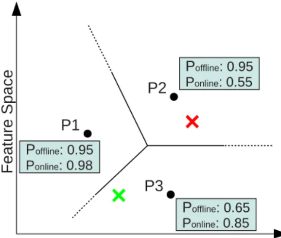
Figure 3.1: Probability estimation- Prin-ciple of using Voronoi cells for probability esti-mation based on feature sub-spaces.

The solution presented here is based on the method proposed by Giacinto & Roli [32]. His learning system uses an input space that is divided into differ-ent sub-spaces. For each sub-area an approximated probability, that is gen-erated for each classifier, determines which classification result of the dif-ferent classifiers is used. The fig. 3.1 shows an exemplary state of the pro-posed classifier combination system in a 2D feature space. The three proto-types P1-P3 represent the internal state of the on-line classifier. Given a set of

S of prototypes

S =

Pk⊂R2|k= 1, . . . , K (3.1)

the Voronoi cellV R(p, S) of a prototypepis defined by all points inR2 that are closer to the appropriate prototype pthan to all other prototypesq ∈S\ {p} of the setS:

V R(p, S) = \

q∈S\{p}

D(p, q) (3.2)

withD(p, q) defined as:

D(p, q) ={x∈_R2 :|p−x|<|q−x|} (3.3) Fig. 3.1 denotes the resulting Voronoi cell borders by black lines and two sample inputs by the red and green cross. The estimated probabilities for the three cells are shown in the blue boxes. In case of the red sample input, the estimated performance of the off-line classifier is higher than for the on-line classifier, therefore the off-line classifier would determine the resulting class label. The cell of the green input sample belongs to the cell of prototype P3. For this cell the on-line classifier has a higher estimated performance than the off-line classifier and determines the system output. Since the Voronoi cells represent the structure of the on-line classifier, the result of the classifier combination system is given by the prototype label of P3.

This leads to the conclusion that a mapping from the input space to the current sit-uation is necessary and that for each sitsit-uation an approximated probability for each classifier must be determined. The computational cost for the probability estimation and therefore the number of required training views increases with the number of dis-crete situation states. Using the prototype identifier as situation has different positive aspects: First the number of situations grows with respect to the problem complex-ity. Another aspect is that an incremental prototype based classifier inserts additional nodes into data regions that contain classification errors. So the density of nodes is re-lated to the local problem complexity. This leads to a more sensitive classifier selection in complex classification areas too. A third point is that no additional computational costs arise for the estimation of the current situation.

For that reason a prototype based learning method was selected as a condition for the on-line classifier architecture. Since the probability for each classifier is determined in a separate process, the system is not restricted in the selection of the classifiers

3.1 Learning Architecture

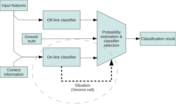
except that one prototype based classifier is necessary. An overview of the interplay between different components building up the proposed learning system can be seen in fig. 3.2. In the case of this thesis the core of the classification architecture holds two separate classifiers. The first classifier was trained in a pre-processing step by off-line learning. The second classifier is used for the on-line training process. An additional

Off-line classifier On-line classifier Situation (Voronoi cell) Classification result Ground truth Input features Context information Probability estimation & classifier selection

Figure 3.2: Working principle of the used learning system - The shown structure clarifies the working principle of the proposed learning sys-tem. This includes the off-line classifier and the on-line classifier. The on-line classifier is able to access additional context information that is not available during off-line training. The state of the on-line classifier is used by the probability estimation for input space partitioning as highlighted by the dashed circle.

selection process selects the appropriate classifier for the current situation. The current situation is given by the active prototype of the on-line classifier. For the initial state of the system, the off-line classifier is pre-trained and is able to achieve generally a better performance than the random initialized on-line classifier. Since the on-line classifier inserts incrementally nodes during the training process, a rising number of Voronoi cells can be used for input space separation and therefore for classifier selection.

3.1.1 Realization

Due to the aims of this thesis, one off-line and one on-line classifier are used. The experiments are based on a Support Vector Machine (Boser et al. [3], LIBSVM [33] implementation) or a Generalized Matrix Learning Vector Quantization and its incre-mental extension (iGMLVQ) as presented in the following section. The on-line clas-sifier is based on an iGMLVQ for all experiments. The off-line clasclas-sifier uses a SVM for the experiments that target artificial data distributions. The experiments targeting traversablilty classification utilize an iGMLVQ on-line classifier. Preliminary tests that compared the performance of GRLVQ, GMLVQ and a version that does not use fea-ture weighting showed that the GMLVQ is able to reach the highest classification rates. These test used different artificial data sets and were also performed using gray-scale object images provided by the COIL-100 [34] image library.

The pre-processing step uses the first data set for the training of the off-line classifier. The off-line classifier used for the experiments based on the artificial data set is a SVM using a radial basis kernel function. The experiments evaluating the performance on the data set that was generated by the use of the simulator uses an iGMLVQ. The off-line classifier is based on the same configuration that was used for the on-off-line classifier, except that this classifier knows just two classes. The off-line training set provides only training patches that belong to the classes of traversable or non traversable objects. The on-line classifier holds three random initialized prototypes, one for each class. Therefore there exist three initial cells that are used for probability estimation. Each new cell is initialized by constant initial values for the probability estimation of the two classifiers. They are selected in such a way that the initial probability values for the off-line classifier are higher than for the on-line classifier. Therefore the off-line classifier it the default option of the initialized system.

During on-line evaluation each given input sample is fed into both classifiers. The prototype id of the on-line classifier is used to determine the active cell and thereby the estimated classifier probability of the off-line and on-line classifier for that cell. The classifier that denotes the highest estimated probability is used to determine the resulting class label. An alternative way of fusing the classifier results was evaluated. There for each classifier and for all three classes probabilities are estimated. They are determined by setting the winner class topestimation given by the activated Voronoi cell

3.1 Learning Architecture

and the two other classes to 1−pestimation

2 . This leads to the three-dimensional vectors

~

ponline and ~pof f line representing one estimated probability per class for each classifier.

Using the Sum-Rule as mentioned in chapter 2 and a normalization to one~ponline+~pof f line

2 leads to the probability vector that represents the result of the classifier combination system. This enhanced combination rule does not have an influence on the classification results, since the classification result can only be affected by the changed combination rule if the estimated probabilities for both classifiers select the same class and the probability of one classifier is very low: 1−ploser

2 −ploser > pwinner − 1−pwinner 2 . The visualization of the classifier results which can be found in section 6.4.4 show the estimated probabilities acquired by this extended method since there an estimated probability for all classes is shown.

The training process updates the probabilities for each classifier according to: pt+1 =p1∗(1−

1

α) (3.4)

if the result of the classifier was not correct or: pt+1 =p1∗(1−

1 α) +

1

α (3.5)

if the result of the classifier was correct. The term _α1 represents the adaptation strength and is defined by α=      50 #samples<50 h #samples> h #samples otherwise (3.6)

With a lower bound for the adaptation strength defined byh. The given sample is used as training example for the on-line classifier if at least one of the three conditions is satisfied:

1. the probability of the on-line classifier is higher than for the off-line classifier pon−line> pof f−line.

2. the classification result of the off-line classifier is wrong.

3. the estimated performance of the best classifier is below a certain threshold pwinner< Qmin.

3.2

GRLVQ and GMLVQ Learning

The generalized Matrix learning vector quantization (GMLVQ) as proposed by Schnei-der et al. [35], [36] is based on the Generalized Relevance Learning Vector Quantization (GRLVQ) as proposed by Hammer & Villmann in [24].

Like all supervised vector quantization based learning methods, a finite training setX = {(xi, yi)⊂Rn× {1, . . . , C} |i= 1, . . . , M} is used to determine a set of K prototypes

W =

w1, . . . , wK and their attached class labels uk ∈ {1, ..., C} that represent the training set. Fore each input samplexsthe winner prototypewk,minhaving the smallest

distance dist (xi, wk) is determined bykmin= argmax k

(dist (xs, wk)). The classification

result is given by the label of the winner prototype uk.

The GRLVQ and GMLVQ minimize the cost function proposed by Sato & Yamada [37] that is given by:

CostGLV Q= X v Φ (µλ(~v)) withµλ(~v) = dλ_r+−dλ_r− dλ r++d λ r− (3.7)

The function Φ is a monotonic function like a logistic function or the identity Φ (x) =x as used here. The termdr+ is the weighted Euclidean distance to the closest prototype with the same label anddr− is the weighted euclidean distance to the closest prototype

with another class label. The GRLVQ uses the weighted euclidean metricdλ =PDv

i=1λi· (vi−wi)2 withλi ≥0 andPiλi= 1. Therefore the distances used in equation 3.7 are

defined by: dλ_r+ = D~v X i=1 λi·(~vi−w~r+,i)2 (3.8) and dλ_r− = D~v X i=1 λi·(~vi−w~r−,i)2 (3.9)

Minimizing of equation 3.7 can be achieved by taking the derivatives with respect to the weighting parameters ∆λ, the best matching correct prototype ∆wr+ _{and the closest} prototype of another class than the training input ∆wr−_{, as shown by Biehl et al. [38].}

This results in the update rules: ∆w~r+=+·Φ0(µλ)·

4·dλ_r−

dλ_r++dλ_r−

3.2 GRLVQ and GMLVQ Learning

for the best matching correct prototype, ∆w~r− =−−·Φ0(µλ)·

4·dλ_r+ dλ

r++dλr−

2 ·Λ (~vj −w~r−,j) (3.11) for the closest wrong prototype and

∆λk=−·Φ0(µλ)·

2·dλ_r−(vk−wr+,k)2−2·dλr+(vk−wr−,k)2

dλ

r++dλr−

2 (3.12)

for the update of the feature weighting.

In comparison to the GRLVQ the GMLVQ is based on an enhanced distance measure-ment. There a matrix is used for distance estimation:

dΛ(ω, ξ) = (ξ−ω)T Λ (ξ−ω) (3.13) Minimizing the same cost function as for the GRLVQ given in equation 3.7 but based on the distance metric given in equation 3.13 results in the modified update rules:

∆~ωr+=+·Φ0 µ ~ ξ · 2·d λ r− dλ_r++dλ_r− 2 ·ΩΩ ~ ξ−~ωr+ (3.14) for the best matching correct prototype,

∆~ωr−=−·Φ0 µξ~· 2·d λ r+ dλ r++dλr− 2 ·ΩΩ ~ ξ−~ωr− (3.15) for the closest wrong prototype and

∆Ωlm =−·Φ0 µ ~ ξ · 2·dλ_r− dλ r++dλr− 2 · h Ω~ξ−w~r+ i m(ξl −w~r+,l) + h Ω~ξ−w~r+ i l ~ ξm−w~r+,m − 2·d λ r+ dλ_r++dλ_r− 2 · h Ω ~ ξ−w~r− i m(ξl−w~r−,l) + h Ω ~ ξ−w~r− i l ~ ξm−w~r−,m ! (3.16) for the update of the feature weighting matrix Λ that is used for the distance estimation given in equation 3.13. It is assumed that Λ is given by Λ = ΩΩ, as shown in Biehl et al. [38].

This enables the classifier to perform a scaling and rotation of the input space, which leads to ellipsoidal clusters that do not need to be aligned to the axes.

3.3

iGMLVQ Extension

As introduced by Kirstein & Wersing [39], an incremental insertion of nodes enables a prototype based network to extend its network complexity to the current problem complexity. Analogous to the implementation of Kirstein & Wersing [39], Kietzmann et al. [40] used this technique to extend the GRLVQ classifier. For the learning system presented here, the same technique was applied for the GMLVQ classifier, resulting in the incremental iGMLVQ classifier.

If there occurs a classification error dr+ < dr− during the training process, an internal

error counter g is increased. If the erroneous sample has a smaller distance dr− to

the wrong prototype than all erroneous samples of that class before it gets saved as a prototype candidate for that class. If a threshold of the number g of occurred errors g > gmax is exceeded, new nodes are inserted. Therefore all prototype candidates that

are collected on classification errors get inserted as new nodes. If there exists a class that had no classification error since the last timegmax was reached, no new prototype

gets inserted for this class. After the node insertion process a reset of the current error countergmax = 0 is performed and the lists of the stored prototype candidates is

cleared.

4

System

This chapter presents the software architecture used for the proposed learning system and the corresponding experiments. The system is partitioned into four sections. The simulation part realizes the generation of data sets and the storage into a database.

Simulator & Data set

generator Data set

Control logic Test framework Performance analysis Data iterator C on te xt ut iliz at io n Image patch Feature extraction Off-line classifier On-line classifier

Probability estimation & classifier selection Reliability matrix Reliability matrix Ground truth D e cis io n m o d u le

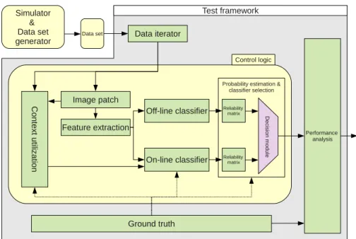
Figure 4.1: Software architecture - The schematic view of the used software architecture. Exchangeable control logic modules allow to test dif-ferent experimental setups using the same test framework. The data sets generated by the simulator are stored for later usage by the experiments.

The second important section of the system contains the infrastructure to execute dif-ferent test runs and to save and visualize the results of the performed tests. This test environment provides an interface to a control logic unit that holds the current experimental configuration. By changing the control logic module, different test config-urations can be realized. The fourth crucial element are the classifier that are hidden inside the control logic. The whole software architecture except the classifier cores are implemented in python using the famous extensions matplotlib and scipy.

Fig. 4.1 shows a schematic overview of the software architecture. It can be seen that the classifier combination system is embedded into the control logic module. In addition to the classifier combination, the control logic handles the image patch generation, the feature extraction and the context utilization. Therefore all processing steps that are relevant for a given experimental configuration are integrated into this module. The surrounding test framework handles the access to the data sets and the extraction of the ground truth. In addition the test framework evaluates the performance of a given control logic element by comparing the ground truth and the estimated class labels. Since the simulator is an external process and the generated data sets are stored externally they are not included in the test framework module. The following sections give an overview over all components that are mentioned in fig. 4.1.

4.1

Simulator

The simulator is used to generate a collection of data sets in a batch process. Each data set entry consists of the following entities:

1. Visual representation 2. Depth map

3. ID map

4. Context information

4.2 Data Sets

4.2

Data Sets

All data sets are stored and can be selected as training or evaluation data set input for the test framework. The samples are presented in the same order to the classifier as they had been recorded during the simulation. This simulates the training data presentation during on-line learning since the acquired training data cannot be shuffled during a real on-line training process.

4.3

Test Framework

The test framework collects all elements that are necessary to build a complete classi-fication framework. For each experiment the same test framework is used. It controls the iteration through the training and test data sets. The resulting functionality is mainly defined by the referenced control logic. The framework controls all inner units to realize the desired system behavior.

4.3.1 Data iterator

The data iterator iterates over all data set entries. Therefore it takes an iteration step width which defines the number of used training samples. The recorded data sets used for the experiments presented in this thesis consist of 3000 recorded samples.

4.3.2 Performance analysis

The Performance analyzer collects all generated output values and is able to visualize them as a graph or store them in a log file. Sample patches that show multiple objects that belong to different classes are neglected and not used for the estimation of the system performance.

4.3.3 Ground truth

The ground truth module determines the correct class labels. Therefore it uses the depth-map and the ID-map provided by the data iterator. The result is a three-dimensional output matrix holding binary values that carry the class affiliation of each patch. This module selects only patches that have a clear class affiliation. This is realized by ignoring patches that represent two or more different classes. Additionally

the module tries to balance the number of training views between the traversable and the other classes since traversable ground patches dominate the recorded data. This is realized by selecting the same amount of patches of the traversable and the ignorable obstacle classes.

4.3.4 Control logic

The control logic module implements the core of the desired learning system behavior. Different configurations allow the simulation of different combination systems. Addi-tionally a PCA-estimator module was realized to determine the principal components of a given data set used by the feature extractor module.

4.3.4.1 Image patcher

The image patcher is used to split the input images into rectangle image patches. These image patches are not overlapping and the desired size can be configured by adjusting external parameters.

4.3.4.2 Feature extraction

The feature extraction is based on the PCA dimensionality reduction. Therefore a pre-processing step is used to determine the eigenvectors and eigenvalues of the input patches of a training data set. The three eigenvectors having the biggest eigenvalues are then used to transform the high-dimensional image patch into a three-dimensional feature vector.

4.3.4.3 Context utilization

A further pre-processing step is used to select the desired input features. That can include the three-dimensional visual features, position information, rotation informa-tion and time informainforma-tion that was used during simulainforma-tion of the ambient light. The selected features are then transformed to get a variance of one and zero mean.

4.3.4.4 Off-line classifier

The off-line classifier only uses the visual features for training. A pre-processing step is used to train this classifier with respect to an off-line training set. The resulting

4.3 Test Framework

performance of the off-line classifier represents the baseline of the whole classification system since the initial configuration prefers the result of the off-line classifier.

4.3.4.5 On-line classifier

The on-line classier is only used during the on-line training process. As described in chapter 3 it is based on a prototype representation that incrementally inserts new nodes. The id of the closest prototype is used by the decision module to determine the estimated probabilities of both classifiers for different sub-spaces of the input data.

4.3.4.6 Reliability matrix

This module estimates the probabilities for each classifier and generates an reliability matrix including a three-dimensional vector for each given input patch of one input frame. For the experiments used here just the winning class is interesting. So the dimension of the winner class is set to the estimated probability pestimation whereas

the other two dimensions are set to 1−pestimation

2 . This guarantees that the sum of the probability of all classes equals one.

4.3.4.7 Decision module

The decision module selects the entry having the highest estimated probability. The result of the selected classifier represents the final output of the classifier combination system.

5

Abstract Data Set

This section explains the experiments that have been realized using two different ar-tificial data sets. Each data set is based on three classes to simulate the required classes: Traversable, non traversable and ignorable obstacles. For the first experiment the off-line classifier is trained on the traversable and non traversable data and only the on-line classifier makes use of the additional ignorable class. The first experiment compares classification results between 2D and 3D data. This was used to simulate the availability of additional feature dimensions to the on-line classifier. In contrast to the first experiment, the second experiment refers a data set that has a more complex data structure for the on-line and the off-line classifier. This experiment was done to highlight the benefits of the proposed classifier combination concept.

5.1

Artificial Data Set I

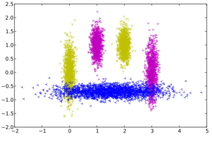
The data set used for the first experiment was generated by five different multivariate Gaussian distributions. Fig. 5.1 shows the arrangement of all three classes. All data points are divided into two subsets, one for training and one for evaluation. The class that is additionally used for the on-line training process is color coded by blue. The two other classes are used for on-line and off-line training. It can be seen that the blue class is not separable from the other classes in a 2D space. Therefore two versions of the data set have been used, the first uses the non separable 2D configuration and a second version uses an additional dimension that represents the context information. As shown in fig. 5.2 the blue class is separable in the third dimension since there are

no overlapping distributions in this space. This configuration was chosen to simulate contextual information if non separable input data can be separated by the use of an additional feature dimension.

2 1 0 1 2 3 4 5 2.0 1.5 1.0 0.5 0.0 0.5 1.0 1.5 2.0 2.5

Figure 5.1: Artificial data set I visualization XY - Each color codes one class. The off-line classifier is only trained on class one(yellow) and two (magenta). The off-line classifier operates also on one additional third class(blue). It can be seen that the third class cannot be separated from the other classes in the 2D space due to the overlapping areas at [0,-0.75] and [3,-0.75]

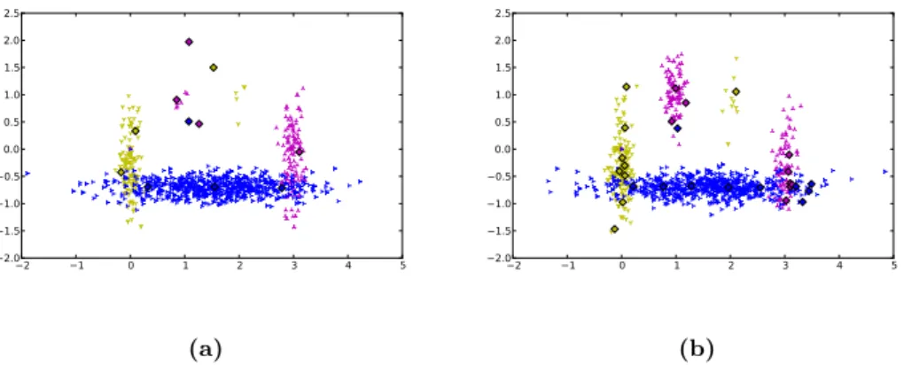
The final state of the on-line classifier at the end of a training process that used 2900 samples is shown in fig. 5.3. The comparison of the training results achieved by using the 3D data set to the results of the 2D data set reveals that the network contains fewer nodes in the case of the 3D data set. Especially the sub-areas of the overlapping regions of the classes have a much denser node distribution. This effect results by the fact that it is not possible for the classifier to separate the two classes. Therefore the classification error rate cannot decrease any more at a certain time and this leads to more incremental node insertions.

5.1 Artificial Data Set I

2

1

0

1

2

3

4

5

1.5

1.0

0.5

0.0

0.5

Figure 5.2: Artificial data set I visualization XZ - Each color codes one class. The off-line classifier is only trained on class one(yellow) and two (magenta). The off-line classifier operates also on one additional third class(blue). 2 1 0 1 2 3 4 5 2.0 1.5 1.0 0.5 0.0 0.5 1.0 1.5 2.0 2.5 (a) 2 1 0 1 2 3 4 5 2.0 1.5 1.0 0.5 0.0 0.5 1.0 1.5 2.0 2.5 (b)

Figure 5.3: Artificial data set I node distribution- Both figures show the distribution of nodes at the end of 2900 training steps. The left figure (a) shows the result of the training using the 3D data set and the right figure (b) shows the result of the training using the 2D data set(third dimension is zero for all data points). The visualized data points represent those samples that were used for the training of the on-line classifier.

Since fig. 5.3 shows only those data points that are used for on-line classifier training, it can be seen that the on-line classifier uses a smaller potion of the two classes centered at [1,1] and [2,1] of the 3D data set. But due to the simple structure of the data set, the on-line classifier has seen samples of all distributions and has inserted sufficient nodes to represent the whole data set. This leads to the conclusion that this experiment does not show the benefits of an additional off-line classifier.

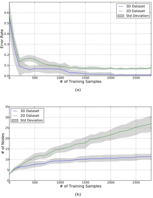
The evaluation of the error rate reveals that the classifier system using the 3D data set for on-line learning is able to reach a higher classification rate. The results are shown in fig. 5.4(a) This shows that the classification system is able to benefit from the additional feature dimensions. The error rate at the beginning of the training process (0 presented training samples) marks the base line and the performance reached by the off-line training.

For this experiment the error rate after off-line training is over 0.5, this is caused by the blue class that is not available to the training process of the off-line classifier. The investigation of the development of the number of nodes during the training process confirms the assumption that the problem of class separation leads to an unlimited node insertion of the incremental training process in case of the 2D data set. This can be seen in fig. 5.4(b), the graph shows the number of inserted nodes of the on-line classifier. The comparison between a classifier training using the 2D and the 3D data set shows that the node insertion rate is not declining during training using the 2D data set.

5.1 Artificial Data Set I 0 500 1000 1500 2000 2500

# of Training Samples

Error Rate

3D Dataset

2D Dataset

Std Deviation

# of Training Samples

# of Nodes

3D Dataset

2D Dataset

Std Deviation

Figure 5.4: System evaluation during training with artificial data set I- The figure (b) shows the number of incremental inserted nodes of the on-line classifier. The blue graph shows the results of the training using the 3D data set and the green graph represents the results using the 2D data set. The gray area surrounding the graphs indicates the standard deviation of the results. The results represent the average ofn= 10 runs.

5.2

Artificial Data Set II

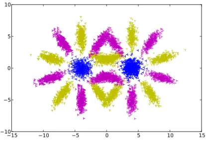
The second experiment is based on a more complex data set configuration. The data set is based on 21 different multivariate Gaussian distributions. They are arranged into two symmetric star like configurations. The additional blue class has much less overlap and is located at the center of the right star as shown in fig. 5.5. In comparison to the first experiment there exists no 3D version of this data set.

15 10 5 0 5 10 15 10 5 0 5 10

Figure 5.5: Artificial data set II visualization - Each color codes one class. The left star configuration was used for off-line classifier training. This includes all three available classes in comparison to the first experiments that used only the classes one(yellow) and two (magenta) have been used for off-line classifier training. For on-line learning the complete data set was used.

The left star configuration was used for off-line classifier training and for on-line training the whole data set was used. The data set was divided into two separate chunks for training and evaluation in the same way as for the first experiment. Since the used classifiers are prototype based, a symmetric arrangement of distributions has no effect on the classifier performance. The results of the evaluation of the error rate during the

5.2 Artificial Data Set II

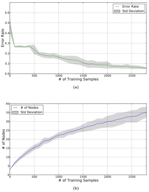
training process is shown in fig. 5.7(a). It can be seen that the on-line training process is able to improve the classification rate for this more complex scenario in the same way as for the much simpler data set used for experiment I.

0 500 1000 1500 2000 2500 3000

# of Training Samples

Error Rate

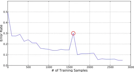
Figure 5.6: Single run system evaluation - This figure shows the de-velopment of the error rate during one training process. The insertion of nodes can have a negative effect on the performance development. The red circle marks an error rate peak between 1500 and 1750 presented samples.

The development of number of nodes during training is shown in fig. 5.7(b), where it can be seen that the node insertion rate declines over time. Due to the complex structure of the data set and that it is not possible to find a perfect separation of all distributions (overlapping) there are still node insertions until the end of the training process. The investigation of the evaluation of one single run reveals that it is possible to achieve a performance degradation during training, as shown in fig. 5.6. The short performance decrease between 1500 and 1750 presented training samples (marked by red circle) is caused by the node insertion process. Since the system assigns default performance values to newly inserted nodes it takes some training samples adjacent to that newly inserted node to adapt the estimated performance values. The configuration of the nodes at the time of the performance decrease is shown in fig. 5.8(d). In comparison to the system configuration before the performance decrease occurs in fig. 5.8(c) it can be seen that a new yellow node was inserted at the position [0.2, -0.25]. The selection

0 500 1000 1500 2000 2500

# of Training Samples

Error Rate

Error Rate

Std Deviation

# of Training Samples

# of Nodes

# of Nodes

Std Deviation

Figure 5.7: System evaluation during training with artificial data set II- The top figure (a) shows the development of the system performance during training. The bottom figure (b) shows the number of incrementally inserted nodes of the on-line classifier. The gray area surrounding the graphs indicate the standard deviation of the results. The results represent the average of n= 10 runs.

5.2 Artificial Data Set II 15 10 5 0 5 10 15 10 5 0 5 10 (a) 15 10 5 0 5 10 15 10 5 0 5 10 (b) 15 10 5 0 5 10 15 10 5 0 5 10 (c) 15 10 5 0 5 10 15 10 5 0 5 10 (d)

Figure 5.8: Prototype representation of the artificial data set -The four images illustrate the prototypes of the on-line classifier at different training states, moreover the given training samples are plotted. The color indicates the class label of each training sample. The first image (a) shows the state at the beginning of the training process, at this time the system had processed only 200 presented samples. (b) shows the state at the end of the training and after presenting 2900 samples. The lower graphs clarify the state of the training system after 1500 (c) and 1600 (d) presented samples. At this time a performance decrease of the overall system occurs. The visualized data points show those samples that were used for the training of the on-line classifier.