A hierarchical multi-label classification ant colony algorithm for protein function prediction

Fernando E. B. Otero · Alex A. Freitas · Colin G. Johnson

A Hierarchical Multi-Label Classification Ant Colony Algorithm

for Protein Function Prediction

Received: date / Accepted: date

Abstract This paper proposes a novel Ant Colony Optimi-sation algorithm (ACO) tailored for the hierarchical multi-label classification problem of protein function prediction. This problem is a very active research field, given the large increase in the number of uncharacterised proteins available for analysis and the importance of determining their func-tions in order to improve the current biological knowledge. Since it is known that a protein can perform more than one function and many protein functional-definition schemes are organised in a hierarchical structure, the classification prob-lem in this case is an instance of a hierarchical multi-label problem. In this type of problem, each example may belong to multiple class labels and class labels are organised in a hi-erarchical structure—either a tree or a directed acyclic graph (DAG) structure. It presents a more complex problem than conventional flat classification, given that the classification algorithm has to take into account hierarchical relationships between class labels and be able to predict multiple class labels for the same example. The proposed ACO algorithm discovers an ordered list of hierarchical multi-label classifi-cation rules. It is evaluated on sixteen challenging bioinfor-matics data sets involving hundreds or thousands of class labels to be predicted and compared against state-of-the-art decision tree induction algorithms for hierarchical multi-label classification.

Keywords hierarchical multi-label classification· ant colony optimisation·protein function prediction

F. E. B. Otero (

B

Classification is a well-known data mining task, where the goal is to learn a relationship between input values and a sired output [14]. In essence, a classification problem is de-fined by a set of examples, where each example is described by predictor attributes and associated with a class attribute. Generally, it involves two phases. In the first phase, given a labelled data set—i.e. a data set consisting of examples with a known class value (label)—as an input, a classifica-tion model that represents the relaclassifica-tionship between predic-tor and class attribute values is built. In the second phase, the classification model is used to classify unknown examples— i.e. examples with unknown class value.

In the vast majority of classification problems addressed in the literature, each example is associated with only one class value or label and class values are unrelated—i.e. there are no relationships between different class values. This kind of classification problems are usually referred to as flat (non-hierarchical) single-label problems. On the other hand, in hi-erarchical multi-label classification problems, examples may be associated to multiple class values at the same time and the class values are organised in a hierarchical structure (e.g. a tree or a directed acyclic graph structure). From a data mining perspective, hierarchical multi-label classification is much more challenging than flat single-label classification. Firstly, it is generally more difficult to discriminate between classes represented by nodes at the bottom of the hierarchy than classes represented by nodes at the top of the hierar-chy, since the number of examples per class tends to be smaller at lower levels of the hierarchy as opposed to top levels of the hierarchy. Secondly, class predictions must sat-isfy hierarchical parent-child relationships, since an example associated with a class is automatically associated with all its ancestors classes. Thirdly, multiple unrelated classes— i.e. classes which are not involved in ancestor/descendant relationship—may be predicted at the same time.

There has been an increasing interest in hierarchical cl-assification, where in general early applications are found in text classification [7, 33, 36, 37, 39] and recently in protein

function prediction [2, 6, 9, 28, 38]. The latter is a very active research field, given the large increase in the number of un-characterised proteins available for analysis and the impor-tance of determining their functions in order to improve the current biological knowledge. It is important to emphasise that in this context, comprehensible classification models— which can be validated by the user—are preferred in order to provide useful insights about the correlation of protein fea-tures and their functions. Concerning the problem of protein function prediction, the focus of this paper, an example to be classified corresponds to a protein, predictor attributes cor-respond to different protein features and the classes corre-spond to different functions that a protein can perform. Since it is known that a protein can perform more than one func-tion and funcfunc-tion definifunc-tions are organised in a hierarchical structure (e.g. FunCat [34] and Gene Ontology [10] protein functional-definition schemes), the classification problem in this case is an instance of a hierarchical multi-label problem. In this paper we propose a novel ant colony classification algorithm tailored for the hierarchical multi-label classifi-cation problem, extending the ideas of our previous hAnt-Miner (Hierarchical Classification Ant-hAnt-Miner) [28] algori-thm. hAnt-Miner—the first ant colony algorithm for hierar-chical classification to the best of our knowledge—discovers a list of classification rules that can predict all classes from a class hierarchy, independently of their level, but has the limitation of not being able to cope with multi-label data. The proposed algorithm overcomes this limitation and it is evaluated on sixteen bioinformatics data sets, taking into ac-count both the predictive accuracy and simplicity (size) of the discovered rule list. The evaluation consists in compar-ing the proposed algorithm against state-of-the-art decision tree induction algorithms for hierarchical multi-label classi-fication. The data sets employed in this evaluation present challenging problems for any classification algorithm as the number of attributes range from 63 to 551, the number of class labels in the class hierarchy ranges from 456 to 4134 and each example is associated with more than one class la-bel.

The remainder of this paper is organised as follows. Sec-tion 2 reviews the related work. SecSec-tion 3 presents an over-view of the Ant Colony Optimisation metaheuristic and its applications in data mining’s classification task. The details of the proposed hierarchical multi-label classification algo-rithm are presented in Section 4. In Section 5, the evaluation measure based on Precision-Recall curves used in our exper-iments is presented. Section 6 presents the computational re-sults. Finally, Section 7 draws the conclusions of this paper and presents future research directions.

2 Related Work on Hierarchical Multi-Label Protein Function Prediction

Much work on hierarchical classification of protein func-tions has been focused on training a classifier for each class label (function) independently, using the hierarchy to

deter-mine positive and negative examples associated with each classifier [2, 3, 20, 22]. As discussed in [6], predicting each class label individually has several disadvantages, as fol-lows. Firstly, it is slow since a classifier needs to be trained n times (where n is the number of class labels in the hierarchy excluding the root label). Secondly, some class labels could potentially have few positive examples in contrast to a much greater number of negative examples, particularly class la-bels at deeper levels of the hierarchy. Many classification al-gorithms have problems with imbalanced class distributions [19]. Thirdly, individual predictions can lead to inconsistent hierarchical predictions, since parent-child relationships be-tween class labels are not imposed automatically during the training. However, more elaborate approaches can correct the individual predictions in order to satisfy hierarchical re-lationships—e.g. a Bayesian network is used to correct the inconsistent predictions of a set of SVM classifiers in [2]. Fourthly, the discovered knowledge identifies relationships between predictor attributes and each class label individu-ally, rather than relationships between predictor attributes and the class hierarchy as a whole, which could give more insights into the data.

In order to avoid the aforementioned disadvantages of dealing with each class label individually, a few authors have proposed classification algorithms that discover a single glo-bal model which is able to predict class labels at any level of the hierarchy. Kiritchenko et al. [21] present an approach where the hierarchical (possibly multi-label) classification problem is cast as a multi-label problem by expanding the class label set of an example with all their ancestor class la-bels. Then, a multi-label classification algorithm is applied to the modified data set. For some examples, there is still a need for a post-processing step to resolve inconsistencies in the class labels predicted. Rousu et al. [33] presents a kernel-based algorithm for hierarchical multi-label classi-fication based on the maximum margin Markov networks framework, wherein a post-processing is not required in or-der to satisfy hierarchical class labels relationships.

In general all of the above approaches can be seen as a ‘black box’, since the produced classification model cannot be interpreted and validated by the user. As previously men-tioned, comprehensibility plays an important role in protein function prediction. Clare et al. [9] present an adapted ver-sion of the well-known C4.5 deciver-sion tree algorithm, which is able to deal with all hierarchical class labels in the data set at hand at the same time. In their approach, a leaf of the de-cision tree predicts a vector of boolean values, indicating the presence/absence of a particular class label. A recent work by Vens et al. [38] presents three approaches for hierarchi-cal multi-label classification using the concept of predictive clustering trees (PCT) to induce decision trees for hierarchi-cal multi-label problems in the context of protein function prediction: (1) building a decision tree for each class indi-vidually; (2) building decision trees in a top-down fashion, where an example can only belong to a class c if it belongs to the c’s parent class; (3) building a single decision tree that predicts all classes at once. They evaluated these approaches

on twenty-four bioinformatics data sets, from which we have selected sixteen to use in this paper, using as protein func-tional classification schemes the FunCat (tree structure) and Gene Ontology (directed acyclic graph structure). Alves et al. [1] proposes two versions of Artificial Immune Systems (AIS) algorithms for hierarchical multi-label classification using the Gene Ontology functional-definition scheme. AIS are computational systems based on the characteristics— mainly the capability of learning and memory—of biolog-ical immune systems.

Holden and Freitas [17] propose a method to improve the performance of top-down hierarchical classification, wh-erein a hybrid particle swarm optimisation (PSO) / ant colo-ny optimisation (ACO) algorithm is used to select—out of a set of predefined candidate classification algorithms—the best (most accurate) classification algorithm to be used at each node of the class hierarchy. This ‘selective’ top-down approach is based on a previous work presented in [35], where the selection of the best algorithm at each node is done in a greedy fashion, rather than using the PSO/ACO algorithm. In Holden and Freitas [18], different ensembles of rules are built for each level of the class hierarchy—using the training examples at the level—and a PSO algorithm is used to optimise the weights used to combine the predictions of different rules in a top-down fashion. While both works are in the context of hierarchical classification, they have been applied to hierarchical single-label classification deal-ing with tree-structured class hierarchies. Therefore, they cannot be straightforwardly applied to the data sets used in this paper, which involves hierarchical multi-label classifi-cation dealing with both tree-structured and DAG-structured class hierarchies.

3 Ant Colony Optimisation

Inspired by the behaviour of natural ant colonies, Dorigo and St¨utzle [13] have defined an artificial ant colony metaheuris-tic that can be applied to solve optimisation problems, called Ant Colony Optimisation (ACO). The main idea for the def-inition of ACO came from the fact that many ant species, even with limited visual capabilities or completely blind, are able to find the shortest path between a food source and the nest. It was discovered that most of the communication among individual ants is based on the use of a chemical, called pheromone, that is dropped on the ground. As ants walk from a food source to the nest, pheromone is deposited on the ground, creating in this way a pheromone trail on the path used. Shorter paths will be traversed faster and, by consequence, will have stronger pheromone concentration than longer paths over a given period of time. The more pheromone a path contains, the more attractive it becomes to be followed by other ants. Hence, as time goes by, more and more ants will prefer the shorter path, which will have more and more pheromone. In the end, (almost) all ants will be following a single path, which usually will represent the shorter path between the food source and the nest.

Ant Colony Optimisation algorithms simulate the beha-viour of real ants using a colony of artificial ants, which co-operate in finding good solutions to optimisation problems. Each artificial ant, representing a simple agent, builds can-didate solutions to the problem at hand and communicates indirectly with other artificial ants by means of pheromone values. At the same time that ants perform a global search for new solutions, the search is guided to better regions of the search space based on the quality of solutions found so far. The algorithm converges to good solutions as a result of the collaborative interaction among the ants; an ant probabilis-tic chooses a trail to follow based on heurisprobabilis-tic information and pheromone values, deposited by previous ants. The in-teractive process of building candidate solutions and updat-ing pheromone values allows an ACO algorithm to converge to optimal or near-optimal solutions. The main aspects of an ACO algorithm are as follows:

– problem representation: the problem is mapped to a gra-ph representation that is used by the artificial ants to build solutions. Ants perform randomized walks on a graph Gc= (C,L), where the set C represents the

ver-tices of the graph and the set L represent the edges be-tween the vertices, in order to build solutions. The graph

Gcrepresents the problem search space;

– building solutions: each ant incrementally builds a can-didate solution by moving through neighbour vertices of the graph Gc. The vertices to be visited are chosen in

a stochastic decision process, where the probability of choosing a particular vertex depends on both the amount of pheromone (τ) associated with the vertex (or the edge leading to the vertex) and a problem dependent heuristic information (η). Hence, a candidate solution is repre-sented by a trail in the graph Gc;

– indirect communication: after building a candidate solu-tion, an ant evaluates the solution in order to decide how much pheromone to deposit in the solution’s trail. In gen-eral, the amount of pheromone deposited is proportional to the quality of the candidate solution. The deposit of pheromone increases the probability that vertices/edges used in a solution will be used again by different ants. ACO algorithms have been successfully applied to sev-eral different flat (non-hierarchical) classification problems, as reviewed in [15]. The first implementation of an ACO algorithm for discovering classification rules, named Ant-Miner, was presented in [29] and more recently variations were proposed in [25, 26, 27, 28]. Ant-Miner, and conse-quentially its variations, combines a traditional machine le-arning’s sequential covering approach with an ACO-based classification rule induction procedure. The sequential cov-ering approach consists of an iterative process of creating on-rule-at-a-time, removing examples from the training set until there are no uncovered training examples (i.e., training examples not classified by any of the created rules). Follow-ing the sequential coverFollow-ing approach, a rule is created usFollow-ing an ACO procedure at each iteration of the process in Ant-Miner.

Despite the Ant-Miner variations for flat classification proposed in the literature, extending Ant-Miner to hierar-chical multi-label classification problems is a research topic that has not yet been explored by other authors, to the best of our knowledge. In the context of hierarchical and multi-label classification, there are two Ant-Miner variations which are worthy of mentioning.

Chan and Freitas [8] proposed a new ACO algorithm, named MuLAM (Multi-Label Ant-Miner), for discovering multi-label classification rules. In essence, MuLAM differs from the original Ant-Miner in three aspects, as follows. Firstly, a classification rule can predict one or more class attributes, as in multi-label classification problems an exam-ple can belong to more than one class. Secondly, each itera-tion of MuLAM creates a set of rules instead of a single rule as in the original Ant-Miner. Thirdly, it uses a pheromone matrix for each class value and pheromone updates only oc-cur on the matrix of the class values that are present in the consequent of a rule. In order to cope with multi-label data, MuLAM employs a criterion to decide whether one or more class values should be predicted by the same rule.

Otero et al. [28] proposed an extension of the flat classi-fication Ant-Miner algorithm tailored for hierarchical clas-sification problems, named hAnt-Miner (Hierarchical Clas-sification Ant-Miner), employing a hierarchical rule eval-uation measure to guide pheromone updating, a heuristic information adapted for hierarchical classification, as well as an extended rule representation to allow hierarchically-related classes in the consequent of a rule. However, hAnt-Miner cannot cope with hierarchical multi-label problems, where an example can be assigned to multiple classes that are not ancestor/decendant of each other. Since in this paper we focus on extending the ideas of hAnt-Miner into the hier-archical multi-label classification problem, a more detailed overview is presented in Subsection 3.1.

3.1 An Overview of Hierarchical Classification Ant-Miner The target problem of hAnt-Miner algorithm is the discovery of hierarchical classification rules in the form IF antecedent

THEN consequent. The antecedent of a rule is composed

by a conjunction of conditions based on predictor attribute values (e.g. length>25 AND IPR00023=yes) while the

consequent of a rule is composed by a set of class labels in potentially different levels of the class hierarchy respecting ancestor/decendant class relationships (e.g., GO:0005216, GO:0005244—where GO:0005244 is a subclass of GO:000-5216). hAnt-Miner divides the rule construction process into two different ant colonies, one colony for creating antecedent of rules and one colony for creating consequent of rules, and the two colonies work in a cooperative fashion.

In order to discover a list of classification rules, a se-quential covering approach is employed to cover all (or al-most all) training examples. Algorithm 1 presents a high-level pseudocode of the sequential covering procedure em-ployed in hAnt-Miner. The procedure starts with an empty

rule list (while loop) and adds a new rule to the rule list while the number of uncovered training examples is greater than a user-specified maximum value. At each iteration, a rule is created by an ACO procedure (repeat-until loop). Given that a rule is represented by paths in two different construction graphs (illustrated in Fig. 1), antecedent and consequent, two separate colonies are involved in the rule construction procedure. Ants in the antecedent colony cre-ate paths on the antecedent construction graph while ants in the consequent colony create paths on the consequent con-struction graph. In order to create a rule, an ant from the antecedent colony is paired with an ant from the consequent colony (the first ant from the antecedent colony is paired with the first ant from the consequent colony, and so forth), so that the construction of a rule is synchronized between the two ant colonies. Therefore, it is a requirement that both colonies have the same number of ants. The antecedent and consequent paths are created by probabilistically choosing a vertex to be added to the current path (antecedent or conse-quent) based on the values of the amount of pheromone (τ) associated with edges and problem-dependent heuristic in-formation (η) associated with vertices. There is a restriction that the antecedent of the rule must cover at least a user-defined minimum number of examples, to avoid overfitting. Once the rule construction procedure has finished, the rules constructed by the ants are pruned to remove irrelevant terms (attribute-value conditions) from their antecedent— which can be regarded as a local search operator—and class labels from their consequent. Then, pheromone levels are updated using the best rule (based on a quality measure Q) of the current iteration and the best-so-far rule (across all itera-tions) is stored. The rule construction procedure is repeated until a user-specified number of iterations has been reached, or the best-so-far rule is exactly the same in a predefined number of previous iterations. The best-so-far rule found is added to the rule list and the covered training examples—i.e. examples that satisfy the rule’s antecedent conditions—are removed from the training set.

Overall, hAnt-Miner can be regarded as a memetic algo-rithm [23], in the sense that it combines conventional con-cepts and methods of the ACO metaheuristic with concon-cepts and methods of conventional rule induction algorithms (e.g. the sequential covering and rule pruning procedures), as dis-cussed earlier.

3.1.1 Hierarchical Rule Evaluation

hAnt-Miner uses a variation of the hierarchical accuracy

me-asure proposed by [21] in order to evaluate rules constructed by ants. Firstly, the set of predicted class labels Pr of rule r

is extended with the corresponding ancestor labels (Pr′) as

Pr′=Pr∪ {∪li∈PrAncestors(li)} −lroot, (1)

where Ancestors(li)corresponds to all ancestor class labels

Algorithm 1 High-level pseudocode of the sequential covering procedure employed in hAnt-Miner. The rule construction process in

hAnt-Miner involves two separate colonies, one for the creation of the antecedent of a rule and one for the creation of the consequent of a

rule.

input : training examples output: discovered rule list begin

1

training set←all training examples;

2

rule list←/0;

3

while|training set|>max uncovered examples do

4 rulebest←/0; 5 i←1; 6 repeat 7 rulecurrent←/0; 8

for j←1 to colony size do

9

// use separate ant colonies for antecedent and consequent construction

10

rulej←CreateAntecedent() +CreateConsequent();

11

// applies a local search operator

12

Prune(rulej);

13

// updates the reference to the best rule of the iteration

14

if Q(rulej)>Q(rulecurrent)then

15

rulecurrent←rulej;

16 end 17 j←j+1; 18 end 19

U pdatePheromones(rulecurrent);

20

if Q(rulecurrent)>Q(rulebest)then

21

rulebest←rulecurrent;

22

end

23

i←i+1;

24

until i≥max number iterations OR RuleConvergence();

25

rule list←rule list+rulebest;

26

training set←training set−Covered(rulebest,training set);

27

end

28

return rule list;

29

end

30

hierarchy. Then, the hierarchical measures of precision (hP) and recall (hR) are computed as

hP=∑i∈Sr |Ai∩Pr′| |Pr′| |Sr| hR=∑i∈Sr |Ai∩Pr′| |Ai| |Sr| , (2)

where Sris the set of all examples covered by (satisfying the

rule antecedent of) rule r and Ai is the set of actual (true)

class labels of the i-th example. The hierarchical precision (hP) is the average number of true class labels that are pre-dicted by rule r divided by the total number of prepre-dicted class labels across the examples covered by rule r; the hier-archical recall (hR) is the average number of true class labels that are predicted by rule r divided by the total number of true class labels which should have been predicted across the examples covered by rule r. Finally, the rule quality measure

Q is defined as a combination of the hP and hR measures,

equivalent to the hierarchical F-measure, given by

Q=hF=2·hP·hR

hP+hR . (3)

3.1.2 Heuristic Information

Antecedent Heuristic Information As in Ant-Miner, the

he-uristic information used in the antecedent construction graph is based on information theory, more specifically, it involves a measure of the entropy associated with each term (vertex) of the graph. The entropy for a term T is computed as

entropy(T ; S) =

|L|

∑

−p(lk|ST)·log2p(lk|ST), (4)

where p(lk|ST)is the empirical probability of observing the

class label lk conditional on having observed term T in the

set of training examples S and |L| is the total number of class labels. Equation (4) is a direct extension of the heuristic function of the original Ant-Miner [29] for flat classification into the problem of hierarchical classification. Since the en-tropy of a term T of the antecedent construction graph varies in the range 0≤entropy(T)≤log2(|L| −1)(where|L| −1

is the number of class labels in the class hierarchy without considering the root class label) and lower entropy values are preferred over higher values, the heuristic information for a term T is computed as

(IPR001693 = no) (IPR005821 = yes) ’start’ (IPR005821 = no) (length) (IPR001693 = yes) (a) GO:0005215 transporter activity GO:0015075

ion transporter activity

GO:0005342 organic acid transporter activity GO:0005275 amine transporter activity GO:0005216 ion channel activity GO:0008324 cation transporter activity GO:0008509 anion transporter activity GO:0046943 carboxylic acid transporter activity GO:0015171 amino acid transporter activity (b)

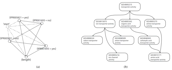
Fig. 1 Examples of the construction graphs employed in hAnt-Miner: in (a) the antecedent construction graph (‘IPR005821’ and ‘IPR001693’ are binary attributes, and ‘length’ is a continuous attribute), where the dummy ‘start’ vertex is unidirectionally connected to all vertices to allow the association of pheromone values on the edge of the first term of the antecedent of a rule; (b) the consequent construction graph, which is defined by the class hierarchy of the problem at hand (in this case, the class hierarchy is represented by a subset of the Gene Ontology’s ion channel hierarchy).

ηT =log2(|L| −1)−entropy(T ; S), (5)

where S is the set of training examples. Equation (5) will give a higher probability of being selected to terms with lower entropy values, which correspond to terms with higher predictive power.

Consequent Heuristic Information The heuristic

informa-tion used in the consequent construcinforma-tion graph is based on the frequency of training examples for each class label of the hierarchy, given by

ηlk =|T Rlk|, (6)

where|T Rlk|is the number of training examples that belong

to class label lk and lk is the k-th class label of the class

hierarchy L.

3.1.3 Using a Rule List to Classify New Examples

In order to classify a test (unseen) example, rules in the dis-covered rule list are applied in a sequential order—i.e. the order in which they were discovered. Therefore, a test ex-ample is classified according to the consequent of the first rule that covers the example. More precisely, the example is assigned the class labels predicted by the rule’s consequent. In the situation where no rule in the discovered rule list covers the test example, a default rule (a rule with an empty antecedent) predicting the set of class labels that occur in all uncovered training examples is used to classify the test example. For example, assuming that there are three un-covered examples e1, e2 and e3, belonging to class labels

{1,1.2,1.2.1},{1,1.2,1.2.2}and{1,1.2,1.2.1,1.2.1.3}, re-spectively. The set of class labels occurring in all uncovered examples comprise the set{1,1.2}, which would be the set of predicted class labels of the default rule.

4 A New Ant Colony Algorithm for Hierarchical Multi-Label Classification

While analysing hAnt-Miner, we have identified the follow-ing limitations. Firstly, the heuristic information, which in-volves a measure of entropy, used in hAnt-Miner is not very suitable for hierarchical classification—i.e. it does not take into account the hierarchical relationships between classes. Although hAnt-Miner’s entropy measure is calculated throu-ghout all labels of the class hierarchy (apart from the root la-bel), each class label is evaluated individually without con-sidering parent-child relationships between class labels.

Secondly, the rule quality measure is prone to overfit-ting. Since only the examples covered by the rule are con-sidered in the rule evaluation, rules with a small coverage are favoured over more generic rules. For example, consid-ering the class label 1.2.1 with 20 examples and two rules that have class 1.2.1 as the most specific class label in their consequent: rule1covering correctly 5 examples out of a

to-tal of 5 covered and rule2covering correctly 19 examples

out of a total of 20 covered. In this case, rule1would have a

higher quality, since all the examples covered by the rule are correctly classified, than rule2, which misclassifies one

ex-ample, though rule2covers all but one examples belonging

to class 1.2.1. One could argue that the rule quality mea-sure of hAnt-Miner could be easily modified to avoid over-fitting by evaluating a rule considering all the examples of its most specific class. The drawback of this approach is that

it favours rules predicting class labels at the top of the hier-archy, since the numbers of examples per class are greater at top class levels. This could potentially prevent the discovery of rules predicting more specific class labels given that the examples covered by a rule are removed from the training set—indeed, this problem was observed in some preliminary experiments.

Thirdly, hAnt-Miner does not support multi-label data since a single path in the consequent construction graph cor-responds to the consequent of a rule. In the case of protein function prediction, where it is known that a protein can per-form more than one function, this is an important limitation. This section presents a new hierarchical multi-label ant colony classification algorithm, named hmAnt-Miner (Hier-archical Multi-Label Classification Ant-Miner), which is ai-med at overcoming the aforementioned limitations. While

hmAnt-Miner shares the same underlying procedure of the hAnt-Miner algorithm, presented in Algorithm 1, it differs

from hAnt-Miner in the following aspects:

– the consequent of a rule is calculated using a determin-istic procedure based on the examples covered by the rule, allowing the creation of rules that can predict more than one class label at the same time (multi-label rules). Therefore, hmAnt-Miner uses a single construction gra-ph in order to create a rule—only the antecedent is rep-resented in the construction graph;

– the heuristic function is based on the Euclidean distance, where each example is represented by a vector of class membership values in the Euclidean space. By using a distance measure, instead of entropy as in hAnt-Miner, it is possible to take into account the relationship between class labels given that examples belonging to related (an-cestor/decendant) class labels will be more similar than examples belonging to unrelated class labels. The use of the Euclidean distance was inspired by a similar use in the CLUS-HMC algorithm for hierarchical multi-label classification [38], which is based on the paradigm of decision tree induction, rather than rule induction. Note that the Euclidean distance is used as the heuristic infor-mation, as well as in the dynamic discretisation proce-dure of continuous attributes;

– the rule quality is evaluated using a distance-based me-asure, which is a more suitable evaluation measure for hierarchical multi-label problems;

– the pruning procedure is not applied to the consequent of a rule. The consequent of a rule is (re-)calculated when its antecedent is modified during pruning, since the set of covered examples might have changed.

4.1 Multi-Label Rule Consequent

Recall that the consequent of a rule in hAnt-Miner is repre-sented as a path in the consequent construction graph, where a trail is a single path from the root class label towards a leaf class label in the class hierarchy. Although the consequent predicts multiple class labels in a hierarchical structure, it

has the limitation of not being able to predict unrelated class labels—i.e. multiple paths in the class hierarchy. One could argue that the consequent could be represented by multiple trails in order to be able to predict unrelated class labels, however it is not clear how to find the optimal combination and number of trails to consider without introducing yet an-other user-defined parameter.

A sensible approach is to use the information available from the examples covered by the rule (i.e. examples that satisfy the rule antecedent) in order to determine the rule consequent. Therefore, the consequent of a rule in hmAnt-Miner is calculated using a deterministic procedure as fol-lows. Given the set of examples Sr covered by a rule r, the

consequent is a vector of length m (where m is equal to the number of class labels in the class hierarchy). The value for each i-th component of the consequent vector for rule r is given by

consequentr,i=

|Sr & labeli|

|Sr|

, (7)

where|Sr & labeli|is the number of examples covered by

rule r that belong to the i-th class of the class hierarchy (labeli). In other words, the consequent of a rule is a

vec-tor where each i-th component is the proportion of covered examples that belong to the i-th class label.

According to Equation (7), each position of the conse-quent vector is a continuous value between 0.0 and 1.0, ra-ther than a presence/absence value of a particular class label. As a result, the value in the i-th component of the consequent of a rule represents the probability of an example that satis-fies its antecedent to belong to the correspondent i-th class of the hierarchy. Figure 2 illustrates the consequent of a rule discovered by hmAnt-Miner; in this example, the predictor attributes in the antecedent of the rule correspond to amino acid ratios from the protein’s sequence and the class labels in the consequent of the rule are represented by Gene Ontol-ogy terms—the number following the colon of a class label in the consequent corresponds to the probability of predict-ing the associated class label.

In order to obtain class label predictions from a rule, it is necessary to select a classification threshold. If the value of the i-th component is greater than or equal to the classifica-tion threshold, the correspondent i-th class label is predicted. Note that the consequents of the rules fulfil the requirements for the hierarchical multi-label classification task: (1) the classes predicted are consistent with the class hierarchy, sin-ce the probability of a parent class label is always equal to or greater than the probability of its children class labels; (2) multiple unrelated classes can be predicted according to the examples covered by the rule.

The same deterministic procedure is applied to compute the consequent of the default rule when classifying an un-seen example, as described in Subsection 3.1.3, with the dif-ference that the uncovered set of examples (i.e., the set of examples which is not covered by any rule) is taken into ac-count in Equation (7).

IF aa_rat_pair_a_h >= 0.053 AND aa_rat_pair_t_c >= 0.1055 AND aa_rat_pair_c_w < 0.0695 AND aa_rat_pair_a_e < 0.2960 AND aa_rat_pair_t_h >= 0.0275 THEN GO0000226:0.10,GO0000943:0.50, GO0001302:0.10,GO0003674:1.00, GO0003676:0.50,GO0003723:0.50, GO0003824:0.50,GO0003887:0.50, ... GO0044464:1.00,GO0045053:0.10, GO0045185:0.10,GO0046907:0.20, GO0051234:0.20,GO0051235:0.10, GO0051649:0.20,GO0051651:0.10

Fig. 2 Example of the consequent of a rule discovered by hmAnt-Miner; in this example, the predictor attributes in the antecedent of the rule correspond to amino acid ratios from the protein’s sequence and the class labels in the consequent of the rule are represented by Gene Ontology terms—the number following the colon of a class label in the consequent corresponds to the probability of predicting the associated class label. Only a subset of the class labels predicted by the rule are shown.

4.2 Distance-based Heuristic Information

According to Subsection 3.1.2, the heuristic information in

hAnt-Miner involves a measure of entropy, as in the

origi-nal Ant-Miner. The entropy characterizes the homogeneity of a collection of examples related to the class attribute val-ues, giving a notion of (im-)purity of the class values’ distri-bution. The more examples of the same class the lower the value of entropy will be and the ‘purest’ is the collection of examples. It should be noted that in all calculations involv-ing entropy, the different class labels (values) are indepen-dently evaluated—i.e. no relationship between class labels is taken into account. In the case of Ant-Miner, which is ap-plied to flat classification problems, the use of the entropy measure does not present a limitation, since there is no re-lationship between class labels. On the other hand, the same cannot be said for hAnt-Miner, which aims at extracting hi-erarchical classification rules, derived from data where the class labels are organised in a hierarchical structure.

To illustrate the limitation of the entropy measure when used in hierarchical problems, let us consider the follow-ing example. Given a tree-structured class hierarchy, where labels {1, 2, 3} are children of the root label and labels

{2.1, 2.2} are children of the ‘2’ label and each class la-bel has 10 examples. Although the entropy is calculated— according to Equation (4)—accross all class labels, the hier-archical relationships are not taken into account. Therefore, the entropy of a hypothetical term ‘IPR00023=yes’ which

is present in 10 examples of class ‘1’ and in 10 examples of class ‘3’ would be the same as of a hypothetical term ‘IPR00023=no’ which is present in 10 examples of class

‘2’ and in 10 examples of class ‘2.1’. The drawback in this

case is that it is known that class labels ‘2’ and ‘2.1’ are more similar than class labels ‘1’ and ‘3’. Hence, it would be ex-pected/desired that the entropy measure (or an alternative heuristic information) exploit hierarchical relationships in order to better reflect the quality of each term in the case of hierarchical classification problems. Intuitively this becomes even more important when dealing with bigger (in terms of number of class labels and depth) hierarchical structures. It should be noted that several Ant-Miner variations—as dis-cussed in [15]—have used a heuristic information based on the relatively frequency of the class predicted by the rule (or the majority class) among all the examples that have a par-ticular term, which would also present the above limitation.

hmAnt-Miner employs a distance-based heuristic

infor-mation, which directly incorporates information from the class hierarchy. More precisely, the heuristic information of a term corresponds to the variance of the set of examples covered by the term (the set of examples that satisfy the con-dition represented by the term). In order to calculate the vari-ance, the class labels of each example are represented by a numeric vector of length m (where m is the number of class labels of the hierarchy without considering the root label). The i-th component of the class label vector of an example is equal to 0 or 1 if the correspondent class label is absent or present, respectively. The distance between class label vec-tors is defined as the weighted Euclidean distance, given by

distance(v1,v2) = s m

∑

where w(li)is the weight associated with the i-th class label,

v1,iand v2,iare the values of the i-th component of the class

label vectors v1and v2, respectively. Then, the variance of a

set of examples is defined as the averaged squared distance between each example’s class label vector and the set’s mean class vector, given by

variance(ST) = |ST| ∑ k=1distance(vk,v) 2 |ST| , (9)

where ST is the set of examples covered by a term T and

v is the set’s mean class label vector. Finally, the heuristic information of a term T is given by

ηT=

variancemax−variance(ST)

variancemax

, (10)

where variancemax is defined as the sum of the worst and

best variance values observed across all terms in order to as-sign values greater than zero to the worst terms, which other-wise would avoid them to be selected by an ant. Note that the heuristic value is normalised so the smaller the value of the variance of a term T the greater its heuristic value becomes. This is analogous to the use of the entropy measure in Ant-Miner and hAnt-Ant-Miner, where smaller values are preferred

over bigger values since they correspond to a more homoge-neous partition (where the great majority of examples belong to the same class).

Recall that the distance function in Equation (8) requires the definition of a class-specific weight. In Vens et al. [38], where the proposed CLUS-HMC algorithm also uses a vari-ance measure based on a weighted Euclidean distvari-ance, sev-eral weighting schemes have been evaluated in the context of hierarchical multi-label classification. As a result of their findings, the preferred weighting scheme—and the one used in hmAnt-Miner—is defined as w(l) =w0· |Pl| ∑ i=1 w(pi) |Pl| , (11)

where w0is set to 0.75 (based on [38]), Pl is the parent class

label set of the class label l and w(pi)is the weight

associ-ated with the i-th parent class label of the class label l. In other words, the weight of a class label l is the multiplica-tion of the w0 weight and the average weight of its parent

class labels. For class labels at the top of the hierarchy (chil-dren of the root label), their weights are set to w0. According

to Equation (11), class labels appearing higher in the hier-archy will have greater weights than class labels appearing lower in the hierarchy. Therefore, concerning the weighted distance function in Equation (8), similarities at higher lev-els of the hierarchy are more important than similarities at lower levels.

4.3 Distance-based Discretisation of Continuous Values As discussed in Subsection 4.2, the entropy measure is not very suitable for hierarchical multi-label classification prob-lems. Therefore, the entropy-based discretisation procedure employed by hAnt-Miner (derived from cAnt-Miner [26]) presents the same limitation of evaluating each of the class labels individually, not taking into account their relation-ships. Consequently, the quality of continuous attributes thr-eshold values are compromised, which can lead to poor dis-covered rules.

Using the variance measure previously defined in Eq-uation (9), hmAnt-Miner employs a distance-based discreti-sation procedure of continuous attributes values in its rule construction process. Given a continuous attribute yi, the

ba-sic idea is to find a threshold value v (where v is a value in the domain of attribute yi) that maximises the variance

gain of both (yi<v) and (yi ≥v) generated partitions of

examples—i.e. the set of examples which have the value of attribute yiless than v and the set of examples which have the

value of the attribute yi greater than or equal to v—relative

to a set of examples S. The distance-based discretisation pro-cedure, dubbed variance-gain discretisation, is divided into two steps as follows.

Let yibe a continuous attribute to undergo the

discreti-sation process and v a value in the domain of yi. The best

threshold value for attribute yi is the value v which

min-imises the variance of both (yi<v) and (yi≥v) generated

partitions of examples from S, maximising the variance gain relative to S as a result, given by

variance gain(yi,v) =variance(S)

−|Syi<v|

|S| ·variance(Syi<v) −|Syi≥v|

|S| ·variance(Syi≥v),

(12)

where|Syi<v|is the total number of examples in the partition

yi<v (partition of training examples where the attribute yi

has a value less than v),|Syi≥v|is the total number of training

examples in the partition yi≥v (partition of training

exam-ples where the attribute yihas a value greater than or equal

to v) and|S|is the total number of training examples. The values of variance(S), variance(Syi<v)and variance(Syi≥v)

are calculated according to Equation (9). The variance gain measure is calculated for all values v, which comprises the average value of each pair of adjacent values vt and vt+1in

the domain of the attribute yi—computed as(vt+vt+1)/2—

and the value v with the highest variance gain associated is then selected as the best threshold value.

Note that the set of training examples S varies accord-ing to the context of the rule construction process, that is to say, the set of training examples S is restricted to the set of training examples covered by the current partial rule being constructed. The only exception to this restriction is when the current partial rule is empty, thus all training examples are used on the evaluation of threshold values. As a result of this restriction, the choice of a threshold value during the rule construction process is tailored to the current candidate rule.

After the selection of the best threshold value v, a rela-tional operator is selected based on the individual variance values of the generated partitions, given by

operator= (_< i f variance(Syi<v)<variance(Syi≥v) ≥ i f variance(Syi<v)>variance(Syi≥v) . (13) According to Equation (13), if the partition of examples

yi<v has a lower variance, then the operator ‘<’ (less-than

operator) is selected; if the partition of examples yi≥v has a

lower variance, then the operator ‘≥’ (greater-than-or-equal-to opera(greater-than-or-equal-tor) is selected; ties are broken at random. As can be noticed, the operator selection has a bias of selecting the more homogeneous partition, given that lower variance val-ues are preferred over higher valval-ues. This is analogous to the bias of the entropy-based discretisation of hAnt-Miner, where lower entropy values are preferred since they are as-sociated with the ‘purest’ partition (the partition with more examples belonging to the same class).

At the end of the discretisation process, a term (a triple

attribute, operator, value) is created to be added to the

cur-rent partial rule (e.g. yi<20) and the rule continues to

un-dergo the rule construction process.

Concerning the computational time complexity of the entropy-based discretisation used in hAnt-Miner and the pr-oposed distance-based discretisation in hmAnt-Miner, the process of finding a threshold value can be divided into two steps. First, both discretisation procedures require the sort-ing of continuous attribute values in order to facilitate the partition of examples. The time complexity of this step is

O(n·log n), where n is the number of training examples un-der consiun-deration.

In the case of the entropy-based discretisation, the sec-ond step involves the evaluation of potentially n candidate threshold values—assuming that each training example has a different value for the continuous attribute undergoing dis-cretisation1—over k different class labels. The complexity of this step is O(n·k), and the total complexity of the entropy-based discretisation is O(n·log n) +O(n·k).

In the case of the distance-based discretisation, the sec-ond step involves the calculation of the mean class label vector for each partition of training examples. This calcu-lation has time complexity of O(n·k). Furthermore, it in-volves the calculation of the distance between each exam-ple’s class label vector and the partition mean’s class label vector in order to determine the variance of the partitions. Since each class label vector has k positions and there are potentially n candidate threshold values, the time complex-ity of the variance calculation is O(n·k). Given that for each candidate threshold value, the mean class label vectors of the partitions must be recalculated because a partition’s exam-ple distribution varies according to the threshold value, the total time complexity of the distance-based discretisation is

O(n·log n) +O([n·k]2_).

Intuitively, if both complexity notations are simplified by dropping the common element O(n·log n), the entropy-based discretisation growing factor is linear in relation to

n·k, while the distance-based discretisation growing factor

is quadratic in relation to n·k. Therefore, the distance-based

discretisation is more computationally complex than the ent-ropy-based discretisation. It should be noted that the number of training examples n covered by a rule, and consequently the potential number of candidate threshold values, tends to decrease in relation to the number of terms in the antecedent of a rule. Hence, the efficiency of the discretisation proce-dure is increased at later stages of the rule construction pro-cess, since less candidate threshold values have to be evalu-ated.

1 _{This represents the worse case scenario for the discretisation}

pro-cedure, and in general, the number of candidate threshold values is smaller than the number of training examples.

4.4 Hierarchical Multi-Label Rule Evaluation

Following a similar approach of using a distance-based mea-sure for the discretisation of continuous values, the variance gain can be applied to compute a rule quality measure. The basic idea to evaluate a rule r using the variance gain mea-sure is to virtually divide the training set S (where S corre-sponds to the set of all training examples) into two partitions: the set of examples covered by the rule r (Sr) and the set of

examples not covered by the rule r (S¬r). Then, the variance

gain of rule r relative to S can be computed as

variance gain(r,S) =variance(S)

−|Sr|

|S| ·variance(Sr) −|S¬r|

|S| ·variance(S¬r).

(14)

The motivation of using the variance as a rule quality measure is as follows. Firstly, it can naturally cope with hierarchical multi-label data, taking into account the rela-tionships and similarities between class labels. Secondly, it favours rules that partition the training set into a more ho-mogeneous sets of examples. As a result, rules that cover a more homogeneous set of examples, as well as leaving un-covered a more homogeneous set of examples (which should facilitate the discovery of other rules in the future), are pre-ferred.

4.5 Simplified Rule Pruning

Since the consequent of a rule is determined as detailed in Subsection 4.1, hmAnt-Miner does not employ a second co-lony in order to construct the consequent of rules. Therefore, the rule pruning procedure is simplified as follows. The rule is submitted to a removal process of its antecedent’s last term and has its consequent re-calculated, since the set of covered examples could change after the removal of the term. The removal process is repeated until the quality of the rule de-creases when its last term is removed or the rule has only one term left in the antecedent.

Let rulecurrentbe the rule undergoing the pruning, which

is considered the best rule at the beginning of the pruning procedure. At each iteration of the pruning procedure, a can-didate rule ruleiis created by removing the last term of the

antecedent of the current best rulebest and the consequent

of ruleiis computed according to Subsection 4.1. Then, the

quality measure qifor ruleiis computed. If the quality

mea-sure qiis higher than the current best quality qbest, rulei

sub-stitutes rulebest, completing an iteration of the pruning

pro-cedure. This procedure is repeated until rulebest has just one

term left on its antecedent or a candidate rule ruleidoes not

5 Evaluation Measure based on Precision-Recall Curves As mentioned in Subsection 4.1, the consequent of a rule in hmAnt-Miner is a numeric vector, where each component of the vector is the probability associated with predicting a particular class label. If the i-th component value is above a specified classification threshold, then the i-th class label is predicted; otherwise it is not predicted. Instead of arbitrarily selecting a classification threshold value—or a set of thresh-old values—to evaluate a rule list, hmAnt-Miner employs a threshold-independent measure. As discussed by [38], a mo-tivation for employing an evaluation measure independently from a classification threshold is that different contexts may require different threshold settings.

Precision-Recall (PR) curves have been frequently used in information retrieval [24, 32] and more recently in the context of hierarchical multi-label classification [38]. A PR curve plots a precision value against its recall value. The precision value corresponds to the number of correct pdictions divided by the total number of prepdictions; the re-call value corresponds to the number of correct predictions divided by the total number of positive examples—i.e., ex-amples belonging to the predicted class label. One of the advantages of using PR curves as a performance measure is its suitability to cope with highly skewed data sets (data sets with a larger amount of negative examples in contrast to a smaller amount of positive examples) given that the num-ber of negative examples is not involved to calculate pre-cision and recall values—i.e. prepre-cision and recall measures only take into account the number of correct positive predic-tions (true positives), the number of incorrect positive pre-dictions (false positives) and the number of incorrect neg-ative predictions (false negneg-ative). Therefore, the number of correct negative predictions (true negatives) does not influ-ence the evaluation. This is an important characteristic con-cerning hierarchical classification since, as previously men-tioned, classes at the lower levels of the hierarchy have fewer (positive) examples. Therefore, it is more important to mea-sure how well a rule predicts the presence of a particular class label (true positive examples) rather than its absence (true negative examples)—independent of whether the posi-tive examples correspond to the majority class or not for the given class label.

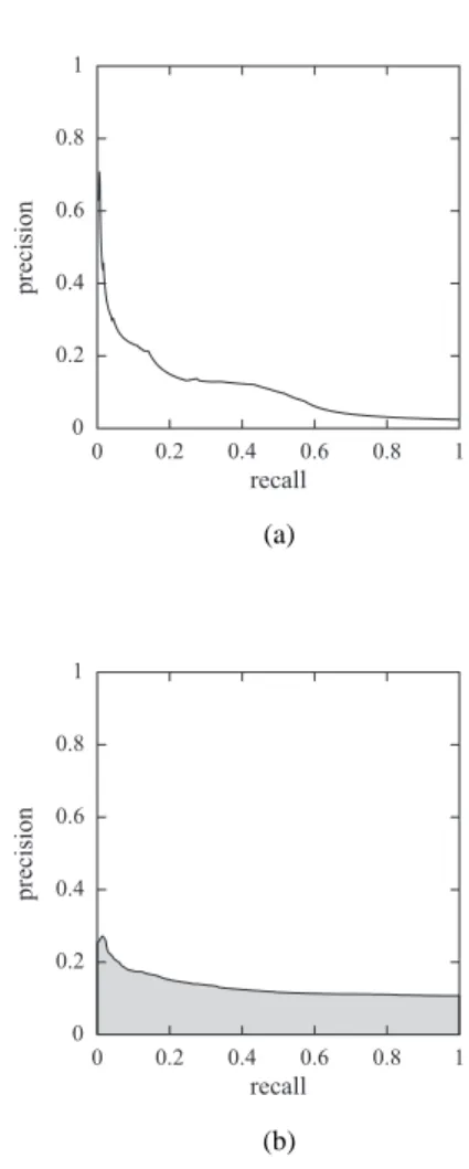
A PR curve, illustrated in Figure 3, is defined by a set of points, where each point corresponds to a pair of preci-sion and recall values for a particular classification thresh-old. Given a classification threshold t, decreasing the value of t from 1.0 to 0.0, different pairs of precision and recall values are obtained. With higher classification threshold val-ues, fewer class labels are predicted (lower recall value) wh-ile the proportion of correct predictions tends to be greater (higher precision value). As the classification threshold is decreased, more class labels are predicted (higher recall val-ues) while the proportion of correct prediction tends to de-crease (lower precision values). Hence, the goal in PR curves is to be on the upper-right-corner, which corresponds to high precision and recall values.

0.8 0.6 0.4 0.2 0.2 0.4 0.6 0.8 0 0 1 1 recall pre ci si on (a) 0.8 0.6 0.4 0.2 0.2 0.4 0.6 0.8 0 0 1 1 recall pre ci si on (b)

Fig. 3 Examples of precision-recall curves: (a) a PR curve showing that higher precision values are generally associated with lower recall values; (b) the shaded area of a PR curve corresponds to the area under the curve measure.

In order to compute the points of a PR curve, and thus calculate the area under the curve, we follow an approach described in [38]. This approach consists in creating an over-all PR curve by micro-averaging precision and recover-all values across all class labels for a range of classification thresholds. The averaged precision (Prec) and recall (Rec) values for a classification threshold t is given by

Prect= ∑i T Pt,i ∑iT Pt,i+∑iFPt,i Rect = ∑i T Pt,i ∑iT Pt,i+∑iFNt,i , (15)

where i ranges over all class labels (excluding the root label, since it is present in all examples), t ranges over all different probability values found in the vector of class labels prob-abilities, and T Pt,i, FPt,i and FNt,i are the number of true

label at the classification threshold t, respectively. The value of Prect corresponds to the number of correct class labels

predictions divided by the number of class labels predicted across all class labels for the given classification threshold

t—i.e., Prect is the proportion of predicted class labels that

are correct. The value of Rect corresponds to the number of

correct class labels predictions divided by the total number of class labels should have been predicted across all class labels for the given classification threshold t—i.e., Rect is

the proportion of the available class labels that are correctly predicted. A pair of Prect and Rect values corresponds to a

point of the PR curve.

Note that points of the PR curve must be interpolated in order to approximate the area under the curve, as discussed in [11]. After determining the points of the PR curve, the area under the PR curve can be approximated by calculating the trapezoidal areas created between each point. Finally, the evaluation measure is defined as the area under the averaged PR curve, denoted as AU(PRC).

6 Computational Results

The proposed hmAnt-Miner algorithm was compared again-st three decision tree induction algorithms for hierarchical multi-label classification proposed in [38]: CLUS-SC, whi-ch consists in inducing a decision tree for eawhi-ch class label in-dividually; CLUS-HSC, which consists in inducing decision trees in a top-down fashion; CLUS-HMC, which consists in inducing a single decision tree that predicts all class labels at once.

We have selected sixteen bioinformatics data sets from Vens et al. [38], which use two different class hierarchy stru-ctures: tree structure (FunCat data sets) and directed acyclic graph structure (Gene Ontology data sets). The directed acy-clic graph (DAG) structure represents a complex hierarchical organisation, where a particular node of the hierarchy can have more than one parent, in contrast to only one parent in tree structures. Table 1 and 2 present details of the data sets used in our experiments. In the experiments conducted by Vens et al. [38], 2/3 of each data set was used for training and the remaining 1/3 for testing. We have used the same training and testing partitions in our experiments.

A summary of the user-defined parameters, their des-criptions and correspondent values, used by hmAnt-Miner is shown in Table 3. We have used the same set of user-defined parameter values in all data sets, which are also considered a standard in the literature [29]; no attempt was made to tune either parameter value for individual data sets. The hmAnt-Miner experiments were performed on a Pentium 4 3.2GHz processor with 1GB of RAM running Linux. Each run of

hmAnt-Miner took on average 2.62 hours (in the range of

0.32 to 6.24 hours, excluding ‘pheno’ data set which took 21 seconds) for FunCat data sets and 12.90 hours (in the range of 1.90 to 21.80 hours, excluding ‘pheno’ data set

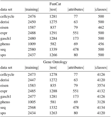
Table 1 Summary of the data sets used in our experiments. The first column (‘data set’) gives the data set name, the second column (‘|training|’) gives the number of training examples, the third col-umn (‘|test|’) gives the number of test examples, the forth column (‘|attributes|’) gives the number of attributes and the fifth column (‘|classes|’) gives the number of classes in the class hierarchy.

FunCat

data set |training| |test| |attributes| |classes|

cellcycle 2476 1281 77 500 derisi 2450 1275 63 500 eisen 1587 837 79 462 expr 2488 1291 551 500 gasch1 2480 1284 173 500 pheno 1009 582 69 456 seq 2580 1339 478 500 spo 2437 1266 80 500 Gene Ontology

data set |training| |test| |attributes| |classes|

cellcycle 2473 1278 77 4126 derisi 2447 1272 63 4120 eisen 1583 835 79 3574 expr 2485 1288 551 4132 gasch1 2477 1281 173 4126 pheno 1005 581 69 3128 seq 2568 1332 478 4134 spo 2434 1263 80 4120

Table 2 The average number of class labels in the hierarchy and the average number of class labels per example of both FunCat and Gene Ontology data sets.

FunCat Gene Ontology average number of classes 489 3932 average labels per example 8.5 34.2

which took 151 seconds) for Gene Ontology data sets.2The data sets with a large number of attributes, namely ‘expr’ and ‘seq’, are the most time consuming in both FunCat and Gene Ontology data sets.

We compared all algorithms in terms of predictive ac-curacy using a measure derived from precision-recall (PR) curves, more specifically the area under the averaged PR curve, denoted as AU(PRC)—discussed in Section 5. Since

hmAnt-Miner is a stochastic algorithm, hmAnt-Miner was

run 15 times—using a different random seed to initialise the search each time—for each data set. Therefore, the value of AU(PRC) reported for each data set corresponds to the aver-age value obtained over 15 runs of the algorithm, followed 2 _{The time taken by CLUSdecision tree induction algorithms is}

re-ported in [38], but in that work a cluster was used, so the time rere-ported in that work cannot be meaningfully compared with the time reported for our experiments in a single processor.

by the standard deviation (average± standard deviation).

For CLUS-SC, CLUS-HSC and CLUS-HMC, the AU(PRC) value for each data set corresponds to the value obtained with a single run of the algorithm, since they are determin-istic algorithms.

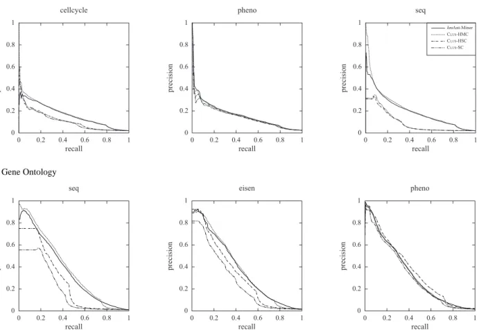
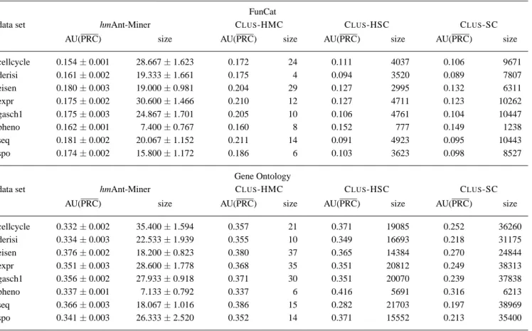
Table 4 shows the AU(PRC) value obtained on the test set by each algorithm and the induced classification model size across all data sets used in our experiments, using Fun-Cat and Gene Ontology, respectively. Figure 4 illustrates a sample of precision-recall curves of hmAnt-Miner, CLUS -HMC, CLUS-HSC and CLUS-SC for ‘cellcycle’, ‘pheno’ and ‘seq’ FunCat data sets and ‘seq’, ‘eisen’ and ‘pheno’ Gene Ontology data sets. As discussed in Section 5, the clos-est to the upper-right corner, the better (more accurate) the curve. For hmAnt-Miner, the classification model size is de-fined as the number of rules discovered; for CLUS-HMC, CLUS-HSC and CLUS-SC the model size is defined as the number of leaf nodes in the induced decision tree, since each path from the root node to a leaf node can be viewed as a rule. In this way, the classification model size for both types of algorithms represents an overall measure of the complex-ity of the model. It should be noted that hmAnt-Miner dis-covers a rule list and the order in which rules are organised is relevant when classifying new examples. Given a new ex-ample, the prediction of its class labels is made by the first rule that covers the example, following the order of the rule list—as detailed in Subsection 3.1.3. Therefore, a particu-lar rule is used only if its previous rules do not cover the example—i.e. if its previous rules have not been used. On the other hand, a decision tree can be converted into a set of rules [30], where the order of rules is not relevant, and therefore each rule can be individually analysed.

Comparison of hmAnt-Miner and CLUS-HSC/SC to CLUS

-HMC: Table 5 presents the summary of the comparisons of the CLUS-HMC algorithm—the algorithm with the best average rank—with the remaining algorithms used in our experiments according to the non-parametric Friedman test with the Holm’s post-hoc test [12, 16] in terms of predic-tive accuracy and classification model size. For each algo-rithm, the average rank and the adjusted p-value obtained by Holm’s post-hoc test are reported using both FunCat and Gene Ontology data sets (‘Combined’ column), using only FunCat data sets (‘FunCat’ column) and using only Gene Ontology data sets (‘Gene Ontology’ column)—the lower the averaged rank, the better the algorithm’s performance.

According to Table 5, there are no statistically significant differences at the 0.01 significance level between hmAnt-Miner and CLUS-HMC, in terms of both predictive accu-racy and classification model size in all of the experiments; CLUS-HMC performs significantly better than CLUS-HSC in terms of predictive accuracy on the FunCat data sets and in terms of both predictive accuracy and classification model size on the combined (both FunCat and Gene Ontology) data sets; CLUS-HMC performs significantly better than CLUS -SC in terms of both predictive accuracy and classification model size in all of the experiments.

Pairwise comparisons between CLUS-HMC/HSC/SC and

hmAnt-Miner: Table 6 presents the summary of all pairwise

comparisons according to the non-parametric Friedman test with the Holm’s post-hoc test [12, 16] in terms of predictive accuracy and classification model size. For each hypothesis (pair of algorithms) tested, the adjusted p-value obtained by Holm’s post-hoc test is reported using both FunCat and Gene Ontology data sets (‘Combined’ column), using only FunCat data sets (‘FunCat’ column) and using only Gene Ontology data sets (‘Gene Ontology’ column).

According to Table 6, the pairwise comparisons do not show statistically significant differences at the 0.01 signifi-cance level between hmAnt-Miner and CLUS-HMC, neither between hmAnt-Miner and CLUS-HSC, in terms of both predictive accuracy and classification model size; hmAnt-Miner is significantly better than CLUS-SC in terms of pre-dictive accuracy in the combined data sets, and in terms of classification model size in all of the experiments; CLUS -HMC is significantly better than CLUS-HSC in terms of predictive accuracy on the FunCat data sets and in terms of classification model size on the combined data sets; CLUS -HMC is significantly better than CLUS-SC in terms of both predictive accuracy and classification model size in all of the experiments.

Summary: The experiments have shown that the proposed

hmAnt-Miner algorithm is competitive with CLUS-HMC—

the most accurate of the CLUSalgorithms—in terms of both predictive accuracy and classification model size. Addition-ally, hmAnt-Miner outperformed CLUS-SC in terms of pre-dictive accuracy on the combined (both FunCat and Gene Ontology) data sets and it has discovered a much simpler classification model than CLUS-SC in all of the experimen-ts. We regard our results as promising, especially consider-ing that the method of inducconsider-ing decision trees usconsider-ing predic-tive clustering trees (PCT)—which is employed by all varia-tions of CLUSalgorithms—has been evolving for more than one decade, with early applications in [4, 31] and more re-cently in the context of hierarchical multi-label classification [5, 6, 38]. On the other hand, the proposed hmAnt-Miner is the first ACO algorithm tailored for hierarchical multi-label classification—to the best of our knowledge—and the ap-plication of ACO algorithms for classification is relatively recent [29].

7 Conclusions

This paper has proposed a novel ant colony algorithm tailo-red for hierarchical multi-label classification, named hmAnt-Miner (Hierarchical Multi-Label Classification Ant-hmAnt-Miner). Extending on the ideas of our previous hierarchical classifi-cation hAnt-Miner algorithm, hmAnt-Miner discovers a sin-gle global classification model, in the form of an ordered list of IF-THEN classification rules, which can predict all class labels from a class hierarchy at once, and examples may be assigned to multiple unrelated class labels. In order