External and Budget Deficits in Developing Countries

Chihi : Department of Economics and CIRPÉE, HEC Montréal, 3000 Chemin de la Côte-Ste-Catherine, Montréal, Québec, Canada H3T 2A7

Phone : 514-340-6735 ; Fax : 514-340-6469

foued.chihi@hec.ca

Normandin : Corresponding author. Department of Economics and CIRPÉE, HEC Montréal, 3000 Chemin de la Côte-Ste-Catherine, Montréal, Québec, Canada H3T 2A7

Phone: 514-340-6841; Fax: 514-340-6469

michel.normandin@hec.ca

Chihi acknowledges the doctoral fellowship of the Tunisian government and financial support from FQRSC. Normandin acknowledges financial support from FQRSC. We thank Hafedh Bouakez and André Kurmann for helpful suggestions.

Cahier de recherche/Working Paper 08-19

External and Budget Deficits in Developing Countries

Foued Chihi Michel Normandin

Abstract:

This paper documents and explains the positive comovement between external and budget deficits for several developing countries. First, the covariance estimated from post-1960 time-series data is numerically positive for each of the 24 countries and statistically significant for almost all cases. This is consistent with previous findings obtained from panel regressions. Second, the empirical covariance is close to that predicted from a tractable small open economy, overlapping generation model with heterogeneous goods. Also, the predicted covariance is induced by shocks which are closely related to internal conditions such as domestic resources and fiscal policies, and to a much lesser extent to external conditions such as the world interest rate, real exchange rate, and terms of trade. This structural analysis explaining the joint behavior of external and budget deficits sharply contrasts with earlier reduced-form studies characterizing the individual behavior of either the external deficit or budget deficit.

Keywords: Covariance decomposition, dynamic responses, internal and external conditions, restricted vector autoregression, small open economy, overlapping generation model with heterogeneous goods.

1. Introduction

The objectives of this paper are twofold. First, we document the comovement between

external and budget deficits for several developing countries. Second, we explain this comovement from a structural model capturing the joint behavior of external and budget deficits.

Earlier studies highlight the existence of a positive comovement for developing countries, as the external balance deteriorates when the budget deficit increases. These analyses mainly rely on panel regressions to extract the comovement that is common across coun-tries. Empirically, the estimated coefficient relating the external deficit to the budget

deficit is always statistically positive (e.g. Calderon, Chong, and Zanforlin 2007; Gruber and Kamin 2007; Chinn and Prasad 2003; Calderon, Chong, and Loayza 2002). A simi-lar effect is recovered from the estimated coefficient relating private saving to the budget

deficit and the identity stating that the current account corresponds to national saving minus investment (Masson, Bayoumi, and Samiei 1998). The robust comovement between external and budget deficits across developing countries sharply contrasts with the het-erogeneous comovement documented for industrial countries (e.g. Boileau and Normandin

2008; Chinn and Prasad 2003).

This paper provides additional evidence of the presence of a positive comovement between external and budget deficits for developing countries. Our analysis relies exclusively on

the time-series of external and budget deficits to extract the comovement that is specific to each country. The time-series are annual observations covering the longest period for the post-1960 era for 24 developing countries. Our primary measure of the comovement

corresponds to the sample estimate of the covariance between external and budget deficits for each country. The findings reveal that this empirical covariance is numerically positive for all countries and statistically significant for many cases. Similar results are obtained

when the comovement is measured by the estimated correlation between external and budget deficits, and the estimated slope coefficient obtained by regressing the external

deficit on a constant and the budget deficit.

Also, previous studies rely on reduced forms to explain either the individual behavior of

the external deficit or budget deficit, rather than their joint behavior. However, combining the results obtained in these studies suggest that the explanation of the positive comove-ment between external and budget deficits from the usual internal and external conditions represents a challenging task. For example, an increase of output implies that the

exter-nal deficit sometimes increases significantly (e.g. Calderon, Chong, and Zanforlin 2007; Calderon, Chong, and Loayza 2002) and sometimes it does not (e.g. Chinn and Prasad 2003), whereas the budget deficit and the governments’ borrowing possibilities are not

significantly affected (e.g. Combes and Saadi-Sedik 2006; Roubini 1991; Berg and Sachs 1988). An increase of the world interest rate induces the external deficit to significantly decreases (e.g. Calderon, Chong, and Loayza 2002), while the probability of rescheduling the public debt statistically increases such that the budget deficit may increase (e.g. Berg

and Sachs 1988). An improvement of the terms of trade implies that the external deficit significantly decreases (e.g. Calderon, Chong, and Zanforlin 2007; Chinn and Prasad 2003; Calderon, Chong, and Loayza 2002), whereas the budget deficit significantly increases (e.g.

Combes and Saadi-Sedik 2006). Finally, an improvement of the real exchange rate uni-formely leads to a significant decline of the external deficit, but the effect on the budget deficit has not been studied so far.

In contrast to early work, this paper relies on a structural analysis to capture the joint be-havior of external and budget deficits. Specifically, we use a tractable small open economy, overlapping generation model with heterogeneous goods to explain the positive

comove-ment between external and budget deficits. The model offers the advantage of involving the external conditions which are often considered for developing countries, such as the world interest rate, real exchange rate, and terms of trade. Also, the model relates the

external and budget deficits to the internal conditions associated with domestic resources and fiscal policies, where these policies may reflect, among other things, changes of the

government’s abilities to collect taxes due to corruption, black markets, or informal mar-kets, for example. Furthermore, the model captures different degrees of imperfectness of intergenerational linkages and financial markets, and as such potential liquidity constraints

faced by developing countries.

The parameters of the model are estimated for each country such that the predicted co-variance between external and budget deficits is close to its empirical counterpart. The predicted covariance is then decomposed into contributions measuring the portions

at-tributable to shocks associated with each internal and external conditions. The contribu-tions with large positive values provide information on the shocks corresponding to prime determinants of the positive comovement between external and budget deficits.

The results reveal that the contributions are almost always positive, so that most shocks induce a positive relation between external and budget deficits for all countries. Also, the magnitude of the contributions indicate that both internal and external conditions play a role in the determination of the comovement between external and budget deficits.

How-ever, the contributions suggest that the shocks associated with internal conditions, and especially domestic resources net of public absorptions, are the most important factors explaining the positive comovement between texternal and budget deficits for most coun-tries. In contrast, the shocks associated with external conditions are dominant for only few

countries. Finally, a robustness analysis confirms that these contributions can be viewed as providing a lower bound of the importance of internal conditions in the determination of the positive comovement between external and budget deficits.

The rest of the paper is organized as follows. Section 2 documents the empirical comove-ment between external and budget deficits for several developing countries. Section 3 presents the model to explain the joint behavior of external and budget deficits. Section 4

elaborates the empirical method to decompose the predicted covariance between external and budget deficits. Section 5 reports the empirical results. Section 6 concludes.

2. Empirical Regularities

This section documents the comovement between external and budget deficits for

develop-ing countries. Our sample includes annual observations coverdevelop-ing the longest period since the post-1960 era for 12 countries in Africa, 7 countries in the Americas, 4 countries in Asia, and 1 country in Oceania. The selections of the countries, frequency, and time pe-riods are dictated by the availability of the data. In particular, there are several missing

values for the budget deficit for many developing countries. The data are fully described in the Data Appendix.

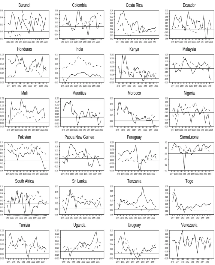
Figure 1 displays the external and budget deficits. The external deficit refers to the negative

of the ratio of nominal current account to nominal gross domestic product. The budget deficit corresponds to the ratio of nominal budget deficit to nominal gross domestic product. Visual inspection of the plots suggests the existence of a positive comovement between

external and budget balances. For many countries, the external and budget positions seem to move in the same direction for most time periods. In general, these movements translate into both external and budget deficits over prolonged horizons. In some cases, however, these movements lead to external balances alternating between deficits and surpluses over

time with persistent budget deficits as for Nigeria, South Africa, and Venezuela.

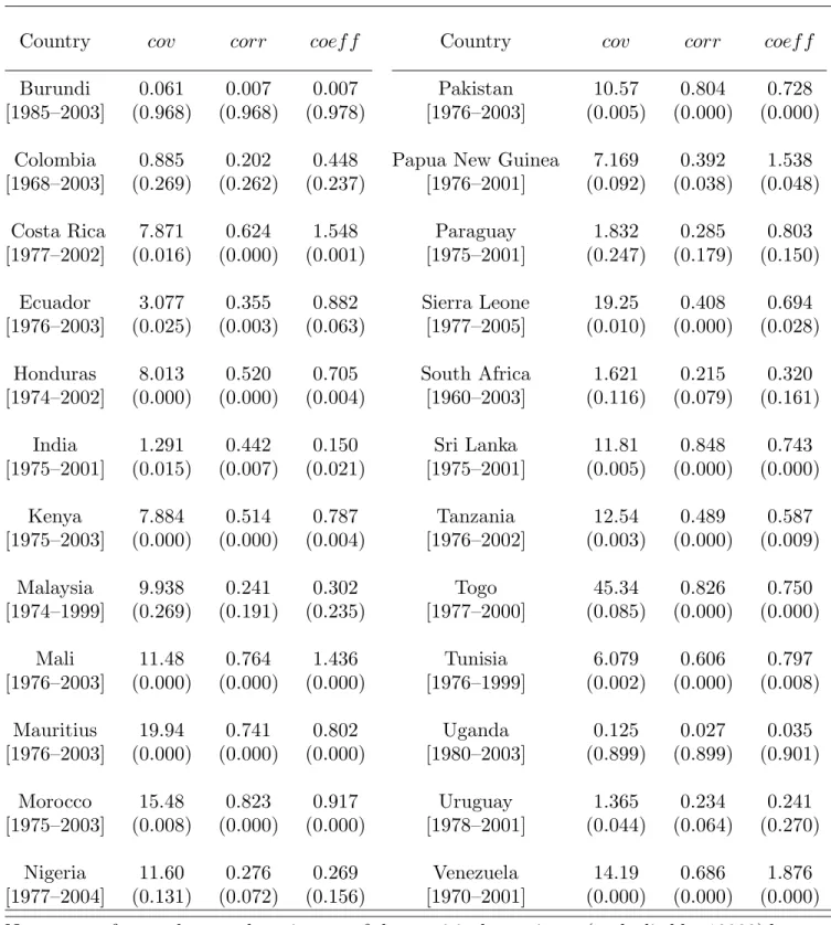
Table 1 reports statistics summarizing the comovements between external and budget deficits. The first statistic is the empirical covariance between external and budget deficits

(multiplied by 10000). Later on, the covariance will prove useful to perform a decomposi-tion allowing the identificadecomposi-tion of the main explanatory factors of the comovement between external and budget deficits. The second statistic is the correlation between external and

budget deficits. Correlations are frequently used in business-cycle studies to document comovements between variables (e.g. Mendoza 1995). The last statistic is the slope co-efficient obtained by regressing the external deficit on a constant and the budget deficit.

Slope coefficients are often used in reduced-form analyses to assess the relation between external and budget deficits (e.g. Chinn and Prasad 2003). All statistics are computed

from the stationary, linearly detrended, external and budget deficits. Similar results are obtained from alternative detrending methods, such as the Hodrick-Prescott filter.

The statistics indicate the existence of a positive comovement between external and budget deficits. For example, the empirical covariance between external and budget deficits is numerically positive for all countries. The covariance averages to 9.559 across all countries; it ranges from a low of 0.061 in Burundi to a high of 45.34 in Togo; and it is larger than

10 for 10 countries, between 5 and 10 for 6 countries, and between 1 and 5 for 5 countries. The covariance is statistically significant at the 1% level for 11 countries, at the 10% level for 6 additional countries, and at the 25% level for 3 more countries.

Also, the correlation between external and budget deficits is numerically positive for all countries. The correlation averages to 0.472 across all countries; it ranges from a low of 0.007 in Burundi to a high of 0.848 in Sri Lanka; and it is larger than 0.75 for 5 countries,

between 0.50 and 0.75 for 6 countries, and between 0.25 and 0.50 for 7 countries. The correlation is statistically significant at the 1% level for 15 countries, at the 10% level for 4 additional countries, and at the 25% level for 2 more countries.

Finally, the slope coefficient relating the external deficit to the budget deficit is numerically positive for all countries. The slope coefficient averages to 0.724 across all countries; it ranges from a low of 0.007 in Burundi to a high of 1.876 in Venezuela; it is larger than 1.00 for 4 countries, between 0.75 and 1.00 for 7 countries, and between 0.25 and 0.75 for 9

countries. The slope coefficient is statistically significant at the 1% level for 12 countries, at the 10% level for 4 additional countries, and at the 25% level for 5 more countries.

Overall, the statistics reveal the existence of a positive comovement between external and budget deficits for many developing countries. This robust result is consistent with previous findings, where the estimated coefficient relating the external deficit to the budget

deficit is statistically positive for panels of developing countries (e.g. Calderon, Chong, and Zanforlin 2007; Gruber and Kamin 2007; Chinn and Prasad 2003; Calderon, Chong, and

Loayza 2002). However, this sharply contrasts with the heterogeneous results documented for industrial countries. For example, the covariance between external and budget deficits is numerically positive for only half of the OECD countries, and the estimated coefficient

relating the external deficit to the budget deficit is no longer significant for panels of industrial countries (e.g. Boileau and Normandin 2008; Chinn and Prasad 2003).

3. The Economic Environment

This section presents the economic environment explaining the joint behavior of external and budget deficits. This environment relies on a structural small open economy,

overlap-ping generation model with heterogeneous goods. The model involves the usual external conditions related to the world interest rate, real exchange rate, and terms of trade, as well as internal conditions such as domestic resources and fiscal policies reflecting changes

of taxes or changes of the government’s abilities to collect taxes. The model also captures different degrees of imperfectness of intergenerational linkages and of financial markets.

In the model, each domestic consumer born at time s sloves in period t the following problem: maxEt ∞ X j=0 βj(1−ρ)jC 1−γ s,t+j 1−γ , (1.1) s.t. Cs,t = h ω1ξ(CT s,t) ξ−1 ξ + (1−ω) 1 ξ(CN s,t) ξ−1 ξ i ξ ξ−1 , (1.2) C_s,tT = h $ζ1_(CH s,t) ζ−1 ζ _{+ (1−$)} 1 ζ_(CF s,t) ζ−1 ζ i ζ ζ−1 , (1.3) (1−ρ)(Bs,t+1+Fs,t+1) = (1 +rt)(Bs,t+Fs,t) +Ys,t−Ts,t−PtCs,t. (1.4)

Equation (1.1) specifies the utility function in terms of private consumption of a composite good. Equation (1.2) defines this consumption in terms of tradable and non-tradable goods.

Equation (1.3) expresses tradable consumption in terms of home and foreign tradable goods. Equation (1.4) depicts the intertemporal budget constraint of the consumer.

All the variables are measured in terms of home tradable goods. Specifically, Cs,t is an index of private consumption, C_s,tN is the consumption of non-tradable goods, C_s,tT is the consumption of tradable goods, C_s,tF is the consumption of foreign tradable goods, and

C_s,tH is the consumption of home tradable goods. Pt, PtN, PtT, PtF, and PtH are the corresponding price indices, with the normalization P_tH = 1. Bs,t is the purchase of one-period bonds issued by the domestic government, Fs,t is the purchase of one-period bonds issued by the foreign government, rt is the world interest rate on one-period bonds,

Ts,t is lump-sum taxes, and Ys,t = Ys,tH +PtNYs,tN is the value of output, where Ys,tH and

Y_s,tN are resources of home tradable and non-tradable goods. The term Et represents the expectation operator conditional on information available in period t.

Also, the parameterβ corresponds to the discount factor,γis the reciprocal of the elasticity

of intertemporal substitution of consumption, ξ is the elasticity of substitution between tradable and non-tradable goods, ζ is the elasticity of substitution between home and foreign tradable goods, ω is the weight of tradable goods in total consumption, and $

is the weight of home tradable goods in total tradable consumption. The parameter ρ is

the probability of being dead next period, or equivalently, the death and birth rates when the population is constant (e.g. Blanchard 1985). Consequently, ρ = 0 indicates that the domestic economy is described by an infinitely-lived representative consumer model, so that agents fully smooth their consumption. Conversely, ρ = 1 implies that the domestic

environment is represented by a sequence of static economies in which each cohort is fully replaced in the subsequent period by a different cohort, such that agents consume only their current income. The parameter ρ may be related to the imperfectness of intergenerational

linkages. In this context, a large value of ρ indicates that consumers are not altruistic, so that agents prefer a consumption profile which is not fully smoothed. Alternatively,ρmay be related to the degree of imperfectness of financial markets. In this case, a large value of

ρindicates that consumers experience difficulties in selling or buying bonds, so that agents are unable to fully smooth consumption through time.

The domestic public sector is described as: (Bt+1+B ∗ t+1) = (1 +rt)(Bt+B ∗ t) +PtGt−Tt, (2.1) = (Bt+Bt∗) +Dt. (2.2)

Equations (2.1) and (2.2) correspond to the intertemporal budget constraint of the gov-ernment. The variables without the subscript srefer to aggregate variables. In particular,

B_t∗ is the aggregate foreign purchases of one-period domestic bonds, Gt is the public con-sumption of goods, and Dt is the budget deficit including the service of the debt.

The external deficit of the domestic economy is measured as the negative of the current account. The current account is:

Zt = (Ft+1−Ft)−(B ∗

t+1−B

∗

t). (3)

Equation (3) defines the current account as the change of net foreign asset positions.

The model (1)–(3) is solved from an analytical approximation. This approximation is fully described in a technical appendix available from the authors. In brief, the individ-ual consumption function is derived, first, from the Euler equation associated with (1.1)

and (1.4) and the distributional assumption of log normality (e.g. Campbell and Mankiw 1989), and, second, from the expected integrated budget constraint associated with (1.4) which is linearized around the means (e.g. Campbell and Deaton 1989). Then, the

ag-gregate consumption function is derived from the individual consumption function and the assumptions that all consumers alive in a given time period face identical taxes and have the same tradable and non-tradable outputs (e.g. Gali 1991). The current account

function is derived from the definition (3), the aggregate budget constraints associated with (1.4) and (2.1), and the aggregate consumption function. To highlight the relation

between external and budget deficits, the current account function is rewritten by sub-stituting aggregate taxes from the expected integrated budget constraint associated with (2.1) and (2.2), which is linearized around the means (e.g. Normandin 1999). Finally, the

consumer price indices associated with (1.2) and (1.3) are log-linearized around the means of exchange rate and terms of trade. The exchange rate is defined as qt = (PtN/PtT). The terms of trade correspond to τt = (PtH/PtF).

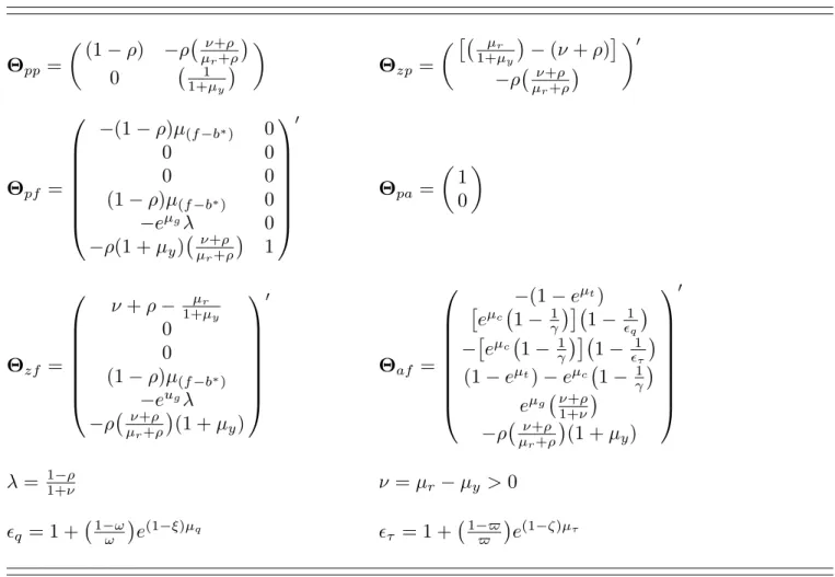
The analytical approximation yields the following first-order vector autoregression (VAR):

x1,t =Θ11x1,t−1+Θ12x2,t, (4) or more explicitly, pt+1 zt = Θpp 0 Θzp 0 pt zt−1 + Θpf Θpa Θzf 1 ft at , with at =ΘafEt ∞ X j=1 λjft+j. (5)

The process (4) corresponds to the rules for the predetermined and nonpredetermined variables. Equation (5) represents the purely forward-looking component of the rules.

All the variables are demeaned. The predetermined variables are pt = ( (ft−b∗t) (bt+b∗t) )

0

, where (ft−b∗t) = (Ft−Bt∗)/Yt−1 and (bt+b∗t) = (Bt+Bt∗)/Yt−1.

The nonpredetermined variable is zt = Zt/Yt. The forcing variables are ft =

(rt ∆ logτt ∆ logqt ∆ logYt loggt dt) 0

, where ∆ is the first difference operator,

gt = PtGt/Yt, and dt = Dt/Yt. The forcing variables include the typical exogenous

stochastic variables for small open economies. These variables reveal information on ex-ternal conditions related to interest rate (rt), terms of trade (∆ logτt), and exchange rate

(∆ logqt), as well as on internal conditions related to domestic resources (∆ logYt), net of public absorptions (loggt), and fiscal policies (dt). Specifically, the budget deficit provides information on taxes, since government expenditures and debt service are given (that is,

gt and rt are exogenous, and (bt +b∗t) is predetermined). Also, the variables zt and dt are consistent with the measures used to document the empirical positive comovement between external and budget deficits (see Section 2). For convenience, at is termed the adjusted current account.

Table 2 relates the coefficients of the rules to the structural parameters and the means of the variables. These coefficients reveal that the rules are static when the probability

of death is unity (ρ = 1, so that λ = 0). In this case, the current account is exclusively affected by contemporaneous output and budget deficit (see the nonzero elements ofΘzf). First, the current account improves following an increase of ouput, through a positive wealth effect. Second, the current account deteriorates following an increase of budget

deficit, since it reflects a tax-cut which leads to an increase of consumption (including that of foreign tradable goods). This translates into a positive relation between external and budget deficits. As explained above, this relation can be due to non-altruistic behavior

associated with imperfect intergenerational linkages or to liquidity constraints related to imperfect financial markets.

In contrast, the rules are dynamic when the probability of death is smaller than one

(0≤ρ <1, so that 0< λ < 1). In this case, the current account is affected by all expected future forcing variables (see the elements of Θaf). First, the current account deteriorates in response to an expected increase of output and an expected decrease of government

expenditures, since this expected increase of resources, net of public absorption, induces an increase of current consumption (including that of foreign tradable goods). Second, when the elasticity of intertemporal substitution of consumption exceeds one, then the

current account may deteriorate in response to an expected decrease of interest rate, an expected appreciation of exchange rate, and an expected deterioration of terms of trade,

through the intertemporal substitution effects associated with an increase of price of future consumption relative to current consumption, an increase of price of future non-tradable goods relative to future tradable goods, and an increase of price of future foreign tradable

goods relative to future home tradable goods. Finally, a positive probability of death implies that the current account deteriorates in response to an expected increase of the budget deficit, whereas a zero probability of death implies that the current account is unaffected because the contemporaneous consumption is unaltered while private saving

increases to reimburse the budget deficit induced by a tax-cut. Hence, a zero probability of death implies that there is no relation between external and budget deficits.

The analytical approximation is completed by constructing the expectations of future forcing variables in (5) from a first-order unrestricted VAR process involving all forcing variables and the adjusted current account (e.g. Boileau and Normandin 2002). This yields

the restricted VAR process:

x2,t =Θ22x2,t−1+Θ2uut. (6)

Here x2,t = (ft0 at) 0

, whereas ut and Θ2uut contain the innovations of the unrestricted

and restricted VARs. Also, Φ22 and Θ22 = Θ2uΦ22Θ

−1

2u include the feedback coefficients of the unrestricted and restricted VARs, whereΘ2u = (e01 . . . e

0

6 Υ)

0

,ek contains the value one for thekth element and zero elsewhere, Υ=ΘafΦ22λ

I−Φ22λ−1, and Iis the identity matrix. Some of the feedback coefficients reflect the dynamic interactions between the contemporaneous budget deficit and the expected forcing variables related to future

internal and external conditions. This response of the budget deficit and the response of the current account (discussed above) to expected movements of future forcing variables may induce a positive relation between external and budget deficits.

Finally, the VARs (4) and (6) are stacked to form the following first-order representation:

or x1,t x2,t = Θ11 Θ12Θ22 0 Θ22 x1,t−1 x2,t−1 + Θ12Θ2u Θ2u ut.

This representation will prove useful to isolate the key factors inducing a positive relation between external and budget deficits.

4. Empirical Method

This section elaborates the empirical method designed to estimate the parameters of system (7) and to identify the main determinants of the positive comovement between external and

budget deficits. Ideally, the empirical method should jointly estimate all the parameters of system (7). In practice, however, this exercise is difficult to perform given the large number of parameters to estimate relative to the number of observations. Specifically, there is a total of 64 parameters which include (i) the means µy, µq, µτ, µr, µg, µd, µ(f−b∗₎,

uc, and ut associated with the variables ∆ logYt, logqt, logτt, rt, loggt, dt, (ft −b∗t), logct = log(PtCt/Yt), and logtt = log(Tt/Yt), (ii) the feedback coefficients incorporated in Φ22 for the unrestricted version of the VAR (6), and (iii) the structural coefficients ρ,

γ, ξ, ζ, ω, and $ involved in the agent’s problem (1). In contrast, the samples for our different countries include between 24 and 44 annual observations per variable.

To circumvent this problem, we apply the following multi-step estimation procedure. The

first step evaluates the means from the sample estimates. The second step determines the feedback coefficients from the OLS estimates. To do so, the variables involved in the unrestricted version of (6) are obtained by using the actual data for forcing variables,

current account, and predetermined variables; by constructing the adjusted current account as at =zt−Θzppt−Θzfft (see the last equation of (4)); and by fixing the means to their estimates and the structural parameter ρ to a given value (see Table 2).

estimates are obtained by setting the covariance between external and budget deficits,cov, to its empirical counterpart (reported in Table 1), by fixing the means and the feedback coefficients to their estimates and by exploting the following moment conditions:

E(cov+ztdt)x02,t−1

= 0, (8)

where x2,t−1 is the vector of instruments, while zt and dt are substituted by the values

predicted by system (7) zt =e03xt =e 0 3 Θxxt−1 + Θuut , (9.1) dt =e 0 9xt =e 0 9 Θxxt−1 + Θuut . (9.2)

To gain intuition, note that the GMM estimates select values for the structural parameters involved in the nonlinear regressioncov =−ztdt+t such that the error term t is orthog-onal to lagged information, where zt anddt are given by (9). Taking expectations implies that E(cov) = −E(ztdt) +E(t) or cov = −σzd provided that the error term is centered on zero, so that the estimated structural parameters ensure that the predicted covariance between external and budget deficit, −σzd, is close to its empirical counterpart, cov. In practice, the GMM estimates are obtained for the structural parameters ρ and γ and for the composite parametersq = 1 + 1−ω_ω

e(1−ξ)µq _and

τ = 1 + 1−$_$

e(1−ζ)µτ_{, given that}

the structural parameters ω,$, ξ, andζ are not individually identified.

The last step of the estimation procedure consists in repeating the second and third steps.

More explicitly, the estimate of ρ obtained in the third step is used in the second step to reestimate the feedback coefficients Φ22. These new estimates ofΦ22 are then used in the

third step to update the estimate ofρ. These iterations are done until the estimates of the

structural parameter ρ and those in Φ22 converge to fix points.

the predicted covariance between external and budget deficits. Specifically, the predicted covariances between variables governed by system (7) are given by:

Σ= ∞ X j=0 Θj_xΘuΩΘ0uΘ j x 0 , (10.1) = ∞ X j=0 ΨjΨ0_j. (10.2)

Here, Σ = E[xtx0_t] is the predicted covariance matrix, Ω = E[utu0_t] = ΛΛ0 is the covariance matrix of innovations, Ψj = ΘjxΘuΛ is the matrix summarizing the

dy-namic responses of various variables j periods after each orthogonal shock, and Λ is a lower triangular matrix transforming the innovations into orthogonal shocks. In prac-tice, Λ is obtained from a Choleski factorization for the ordering x2,t = (ft0 at)

0 and ft = (rt ∆ logτt ∆ logqt ∆ logYt loggt dt)

0

. This ordering ensures that the shocks

related to internal conditions capture the portion that is orthogonal to external conditions. Also, the shock related to loggt corresponds to a shock on the level of government expen-ditures, rather than on government expenditures to output ratio, given that it captures the

portion that is orthogonal to output. Likewise, the shock related to dt is a shock on taxes, since it measures the portion that is orthogonal to output, government expenditures, and interest rates. Finally, the shock affectingat captures any other shocks than those already associated with ft, because it is the portion that is orthogonal to forcing variables.

From expression (10), the predicted covariance between external and budget deficits is decomposed as follows: −σzd=ψr+ψτ +ψq+ψy+ψg+ψd+ψa. (11) The component ψr = P∞ j=0 −e 0 3Ψje4 e0 9Ψje4

is the portion of the predicted covariance between external and budget deficits which is attributable to the interest rate shock. In

practice, this portion is computed by evaluating the sum over 100 years. Also, the portion involves the dynamic responses of the external deficit [i.e. −e0₃Ψje4

] and of the budget deficit [i.e. e0₉Ψje4

] to an interest rate shock. The other terms in (11) are defined in

an analogous way. The components ψτ, ψq,ψy, ψg,ψd, and ψa measure the contributions to the predicted covariance of the terms of trade shock, exchange rate shock, output shock, government expenditures shock, tax shock, and other shocks. The component with the largest positive value provides information on the shock corresponding to the prime

determinant of the positive comovement between external and budget deficits.

5. Results

This section applies the empirical method just described for 12 of our 24 initial countries. The selection of the countries relies on the availability of the data required for the

estima-tion exercise. In particular, the series on public debt are often missing. The data are fully described in the Data Appendix.

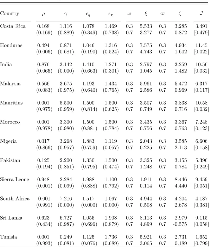
The estimates of all parameters are available upon request. For briefness, Table 3 reports

only the estimates of the structural and composite parameters. The estimates systemati-cally display the expected signs and the appropriate magnitudes, but are often imprecise since the number of estimated parameters is large relative to the sample size. Specifically, the estimates indicate that the probability of death, ρ, is always between zero and one.

Also, the probability of death averages to 0.318 across all countries; and it ranges from a low of 0.001 in Mauritius, Morocco, South Africa, and Tunisia to a high of 0.948 in Sierra Leone. As explained above, large values of ρ may reflect non-altruistic behavior

associ-ated with imperfect intergenerational linkages or liquidity constraints relassoci-ated to imperfect financial markets. Interestingly, previous findings detect strong liquidity constraints for many developing countries (e.g. Haque and Montiel 1989). Among the countries which are

common to our sample, severe liquidity constraints are documented for India, Malaysia, and Nigeria, whereas no liquidity constraint is detected for Morocco. Our estimates accord

with these results, that is, the estimates of the probability of death are substantially larger for India, Malaysia, and Nigeria than that for Morocco.

The estimates imply that the elasticity of intertemporal substitution of consumption, (1/γ), is always positive. Also, the elasticity averages to 0.719 across all countries; and it ranges from a low of 0.139 in South Africa to a high of 4.016 in Tunisia. Interestingly, these estimates are consistent with previous findings, where the estimates of the elasticity are

smaller than unity for almost all selected developing countries (e.g. Ogaki, Ostry, and Reinhart 1996; Ostry and Reinhart 1992; Giovannini 1985).

As expected, the estimates reveal that the composite parameter, q, is always larger than

one. Also, the elasticity of substitution between tradable and non-tradable goods, ξ, is systematically positive — where this elasticity is recovered from the definition q = 1 + 1−ω_ω e(1−ξ)µq_{, given values of the weight ω, and the estimated values of the meanµ}

q. The elasticity uniformely declines as the weight of tradable goods in total consumption,ω, increases. For example, fixing the weight to ω = 0.3 implies that the elasticity averages to 4.589; and it ranges from a low of 1.911 in Sierra Leone to a high of 8.113 in Sri Lanka. In contrast, setting ω = 0.7 implies that the elasticity averages to 1.935; and it ranges from

a low of 0.114 in Sierra Leone to a high of 4.899 in Sri Lanka.

Likewise, the estimates indicate that the composite parameter,τ, is always larger than one. Also, the elasticity of substitution between home and foreign tradable goods, ζ, is almost

always positive — where this elasticity is obtained from τ = 1 + 1−$_$

e(1−ζ)µτ_{, given}

values of the weight $, and the estimated values of the mean µτ. The elasticity decreases as the weight of home tradable goods in total tradable consumption, $, increases. In

particular, fixing the weight to$= 0.3 implies that the elasticity averages to 4.411; and it ranges from a low of 2.731 in Tunisia to a high of 8.446 in Sierra Leone. However, setting

$= 0.7 implies that the elasticity averages to 1.336; and it ranges from a low of -0.575 in

Sri Lanka to a high of 4.440 in Sierra Leone. Overall, the values for the weights, ω and $, and the elasticities of substitution,ξandζ, are consistent with previous findings, where the

estimates of the weight are around 0.5 and the estimates of the elastiticity of substitution between imported and non-tradable goods is about 1.3 across selected developing countries (e.g. Ostry and Reinhart 1992). In these studies, however, the tradable goods are usually

not decomposed into imported and non-imported goods.

For completeness, Table 3 also presents the overidentification restriction tests. The statis-tics, J, reveal that the restrictions associated with the moment conditions (8) are never

rejected at the 1% level, are refuted at the 5% level for only 3 countries, and at the 10% level for 2 additional countries.

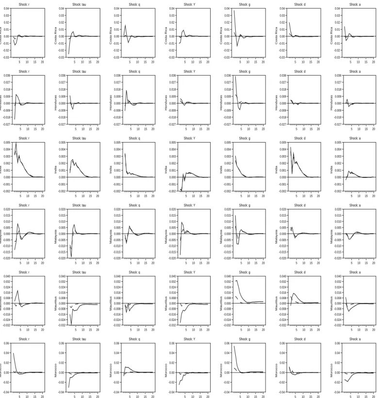
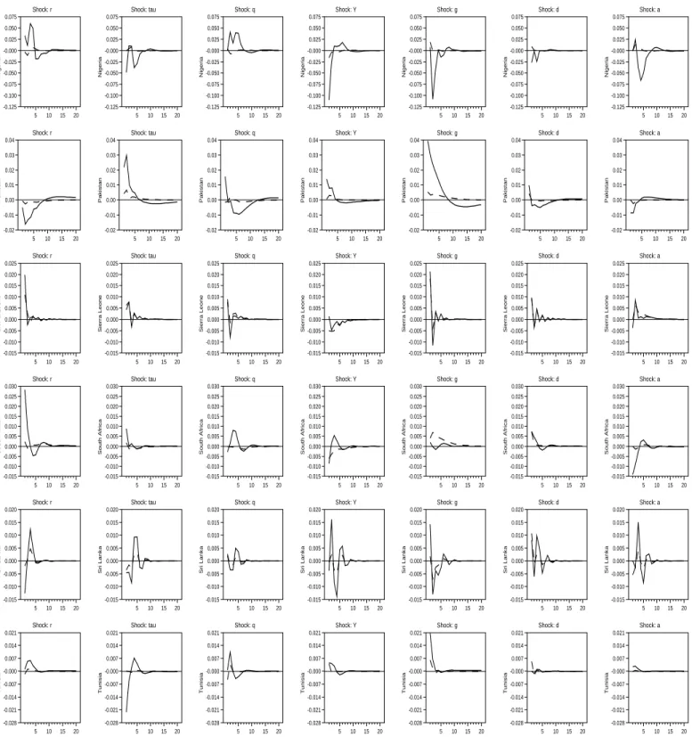
Figure 2 displays the transitory dynamic responses of external and budget deficits

follow-ing, one standard deviation, shocks. These responses are obtained from our benchmark ordering: x2,t = (ft0 at)

0

and ft = (rt ∆ logτt ∆ logqt ∆ logYt loggt dt) 0

. In brief, a positive shock to interest rate leads to positive responses of external and budget

deficits over most horizons, except for Costa Rica, Malaysia, Mauritius, and Pakistan. A positive shock to terms of trade usually produces negative responses of external and budget deficits, except for India, Pakistan, Sierra Leone, Sri Lanka, and South Africa. A positive shock to exchange rate generally implies positive responses of external and budget

deficits, except for Malaysia, Mauritius, and Pakistan. A positive shock to output fre-quently leads to negative responses of external and budget deficits, except for Honduras, Pakistan, Sri Lanka, and Tunisia. A positive shock to government expenditures almost

always yields positive responses of external and budget deficits, except for Nigeria and Sri Lanka. Finally, a positive shock to budget deficit due to a tax cut yields positive responses of external and budget deficits over most horizons, except for Nigeria and Sri Lanka.

Importantly, these dynamic responses provide some intuition behind the predicted relation between external and budget deficits. For example, the various shocks produce responses of external and budget deficits which are almost always of the same sign. This suggests

that most shocks induce a positive relation between external and budget deficits. In turn, these relations translate into a positive predicted comovement between external and

bud-get deficits, as observed in the data. This sharply contrasts with the results obtained from reduced-form analyses, suggesting that the explanation of the empirical positive covari-ance between external and budget deficits from the usual external and internal conditions

represents a challenging task (e.g. Calderon, Chong, and Zanforlin 2007; Combes and Saadi-Sedik 2006; Chinn and Prasad 2003; Calderon, Chong, and Loayza 2002; Roubini 1991; Berg and Sachs 1988).

Also, the various shocks yield responses of external and budget deficits which generally exhibit a modest persistence. That is, most shocks affect the external and budget deficits for a horizon of about 5 years, except for India, Pakistan, and Sri Lanka. This suggests that the different shocks lead to a positive comovement between external and budget deficits

mainly through their short-run effects.

Moreover, the various shocks induce responses of external and budget deficits which display

different magnitudes. For example, a government expenditures shock leads to pronounced responses of external and budget deficits for many countries. These responses are clearly the largest (in absolute values) for Costa Rica, Honduras, and Pakistan. In additions, these responses seem quite large for Mauritius, Morocco, Sierra Leone, and Tunisia. Also,

an output shock induces large responses of external and budget deficits for Nigeria and Sri Lanka. Given the measures involved in our covariance decomposition, these results suggest that shocks to internal conditions represent the prime determinants of the positive

comovements between external and budget deficits for most countries. In contrast, a terms of trade shock yields the largest responses of external and budget deficits for Malaysia, while an interest rate shock produces the largest responses for India and South Africa. These findings suggest that shocks to external conditions constitute the main explanation

of the positive comovements between external and budget deficits for only few countries.

Table 4 confronts the empirical and predicted covariances between external and budget

deficits. These statistics display similar numerical values for almost all countries. Also, the empirical and predicted covariances are statistically identical at all conventional levels

for every country, except Tunisia.

Table 4 further reports the estimates of the contribution of each shock to the predicted

covariance between external and budget deficits. Again, these estimates are computed for our benchmark ordering: x2,t = (ft0 at)

0

and ft = (rt ∆ logτt ∆ logqt ∆ logYt loggt

dt)0. The estimates are always numerically positive, except those associated with the portions attributable to the shocks of exchange rate, tax cut, and other factors (summarized

by the adjusted current account) for Nigeria, and interest rate for Mauritius. The positive contributions of most shocks reflect the notion that the responses of external and budget deficits are frequently of the same sign. Also, these positive contributions reveal that most shocks induce a positive relation between external and budget deficits, translating into a

positive predicted comovement between the two deficits.

The contributions also display different sizes across the various shocks. In general, the

magnitude of the contributions indicate that both internal and external conditions play a role in the determination of the comovement between external and budget deficits. How-ever, the contributions related to the government expenditures shock represent the largest numerical values for 7 out of 12 countries, namely Costa Rica, Honduras, Mauritius,

Mo-rocco, Pakistan, Sierra Leone, and Tunisia. Also, the portions attributable to the output shock are the most important component for 2 countries, that is, Nigeria and Sri Lanka. But the contributions of the budget deficit shock associated with a tax change never

dis-play the largest numerical values. So far, these results reveal that the shocks associated with internal conditions, and especially the domestic resources net of public absorptions, are the most important factors explaining the positive comovement between external and budget deficits for most countries. These findings confirm the intuition deduced from the

dynamic responses.

In contrast, the contributions related to the interest rate shock reach the largest numerical

values for only 2 countries, namely India and South Africa. Also, the portions attributable to the terms of trade shock are the most important component for only 1 country, that

is, Malaysia. In addition, the contributions of the exchange rate shock never exhibit the largest numerical values. In sum, these findings indicate that the shocks associated with external conditions play a major role in the determination of the positive comovement

between external and budget deficits for only few countries.

Note that many estimates of the contributions are precisely estimated. Importantly, se-lecting the contributions with the largest positive, statistically significant (rather than

numerical), values leads to similar results as above. The only differences are the following: the contribution of the shock to output (rather than government expenditures) becomes the most important for Morocco, the portion attributable to the shock to budget deficit

in-duced by a tax change (rather than interest rate) is the most crucial for South Africa, while the contribution of the shock to terms of trade (rather than government expenditures) is the most dominant for Tunisia. Overall, the findings confirm that the shocks associated with internal conditions still constitute the prime determinants of the positive relation

between external and budget deficits for most countries, whereas the shocks related to external conditions remain key factors for few countries.

To check the robustness of the results, Table 5 presents the contributions obtained from the following ordering: x2,t = (ft0 at)

0

andft = (∆ logYt loggt dt rt ∆ logτt ∆ logqt)0. This alternative ordering places the variables related to internal conditions before those associated with external conditions, unlike the benchmark ordering. Accordingly, the

alternative ordering assumes that the internal conditions are more predetermined than the external ones. Importantly, this case may be relevant for many developing economies which heavily rely on natural resources. This is because the endowment of these resources

is crucially affected by exogenous, and possibly highly predetermined, factors. Examples of such factors are weather conditions affecting crops for agricultural economies (i.e. Costa Rica), geological conditions affecting the mining industry (i.e. South Africa), and reserves

of oil affecting the petrolium industry (i.e. Nigeria). All these exogenous factors are captured by shocks to domestic resources, net of public absorption, in our alternative

ordering.

For the alternative ordering, the contributions related to the government expenditures

shock now represent the largest numerical values for 9 out of 12 countries, namely Costa Rica, Honduras, India, Mauritius, Morocco, Pakistan, Sierra Leone, Sri Lanka, and Tunisia. Also, the portions attributable to the output shock are still the most important component

for 2 countries, that is, Nigeria and Sri Lanka. Finally, the contribution of the budget deficit shock associated with a tax change becomes the largest numerical value for South Africa. Consequently, these results indicate that the shocks associated with internal conditions are now the most important factors explaining the positive relation between external and

budget deficits for all countries. Interestingly, these contributions reinforce the conclusion reached from the benchmark ordering. Moreover, the results suggest that the contributions obtained from the benchmark ordering can be viewed as providing a lower bound of the importance of internal conditions in the determination of the positive comovement between

external and budget deficits.

6. Conclusion

This paper documented and explained the positive relation between external and budget deficits for several developing countries. First, we provide evidence of the existence of a

positive comovement between external and budget deficits. This is consistent with previous findings obtained from panel regressions. However, our analysis relies on time-series of external and budget deficits to extract the comovement that is specific to each country. The estimated covariance between external and budget deficits is numerically positive for

all countries and statistically significant for many cases. Similar results are found from the estimated correlation between external and budget deficits, and the estimated slope coefficient obtained by regressing the external deficit on a constant and the budget deficit.

Second, we explain the joint behavior of external and budget deficits from a tractable small open economy, overlapping generation model with heterogeneous goods. This sharply

con-trasts with earlier reduced-form studies characterizing the individual behavior of either the external deficit or budget deficit. Our model offers the advantage of relating external and budget deficits to the external and internal conditions usually considered for developing

economies. The model further captures different degrees of imperfectness of intergenera-tional linkages and of financial markets, and as such potential liquidity constraints faced by developing countries.

Empirically, the model is estimated for each country such that the predicted covariance

between external and budget deficits is close to its empirical counterpart. The predicted covariance is then decomposed into contributions measuring the portions attributable to shocks associated with each internal and external conditions. The size of the contributions indicate that the shocks associated with internal conditions, and especially the domestic

resources net of public absorptions, are the most important factors explaining the positive comovement between external and budget deficits for most countries. In contrast, the contributions of the shocks associated with external conditions are dominant for only few

Data Appendix

This appendix describes the data which are mainly collected from the International Fi-nancial Statistics (IFS), released by the International Monetary Fund. The annual data cover the longest period since the post-1960 era for our selected developing economies. The selections of the countries, frequency, and time periods are dictated by the availability of the data, and in particular of budget deficit and public debt. Table 1 lists the countries and time periods for which external and budget deficits are available. Table 3 lists the countries for which all variables required for the estimation exercise are available.

The variables which are central to our analysis are external and budget deficits. The ex-ternal deficit refers to the negative of the nominal current account in U.S. dollars (source: IFS) converted in domestic currencies from the appropriate nominal exchange rate (source: IFS), divided by the nominal gross domestic product in domestic currencies (source: IFS). The budget deficit is the nominal budget deficit in local currencies (source: IFS), normal-ized by the nominal gross domestic product.

The predetermined variables are the public debt and net foreign assets. The public debt is measured from the nominal foreign and domestic public debts of central governments net of guaranteed loans in domestic currencies (source: IFS), divided by the nominal gross domestic product. The net foreign assets correspond to the nominal net foreign assets in U.S. dollars (source: Lane and Milesi-Ferretti 2006) expressed in domestic currencies, normalized by the nominal gross domestic product. Exceptionally, for Sierra Leone the nominal net foreign assets in U.S. dollars is taken from the World Development Indicators (WDI) published by the World Bank.

The forcing variables are the world interest rate, terms of trade, exchange rate, output, and government expenditures. The world interest rate is proxied by the nominal yield on three-month US treasury bills (source: IFS) minus the expected inflation, constructed as the one-step-ahead forecasts of an ARMA(1,1) process for the annual growth rate of the consumer price index (source: IFS) (e.g. Fry 1986; Uribe and Yue 2006). The terms of trade are measured from the ratio of export prices to import prices (source: WDI). The exchange rate corresponds to the real effective exchange rate (source: IFS). Exceptionally, for Honduras, Mauritius, and Sri Lanka the real effectice exchange rate is taken from Cashin, Cespedes, and Sahay (2004), while for India the real effective exchange rate is

published by the Reserve Bank of India. Output is obtained from the nominal gross domestic product, divided by the consumer price index. The government expenditures are computed as the nominal government expenditures of services, consumption goods, and investment goods in domestic currencies (source: IFS), normalized by the nominal gross domestic product.

The additional variables required for the estimation purpose are taxes and private con-sumption. Taxes correspond to the ratio of the nominal tax revenues in domestic currencies (source: IFS) to the nominal gross domestic product. Private consumption is obtained from the nominal households expenditures of services, nondurable goods, and durable goods in domestic currencies (source: IFS), normalized by the nominal gross domestic product.

All the variables are linear detrended to ensure stationarity. Similar results are obtained from alternative detrending methods, such as the Hodrick-Prescott filter.

References

Berg, A., and J. Sachs (1988) “The Debt Crisis: Structural Explanations of Country Performance,”Journal of Development Economics 29, pp. 271–306.

Blanchard, O.J. (1985) “Debt, Deficits, and Finite Horizons,”Journal of Political Economy 93, pp. 223–247.

Boileau, M., and M. Normandin (2008) “Fiscal Policies, External Deficits, and Budget Deficits: A Multi-Country Analysis,” manuscript, HEC Montr´eal.

Boileau, M., and M. Normandin (2002) “Aggregate Employment, Real Business Cycles, and Superior Information,” Journal of Monetary Economics 49, pp. 495–520.

Calderon, C.A., Chong, A., and N.V. Loayza (2002) “Determinants of Current Account Deficits in Developing Countries,”Contributions to Macroeconomics 2, pp. 1–31.

Calderon, C.A., Chong, A., and L. Zanforlin (2007) “Current Account Deficits in Africa: Stylized Facts and Basic Determinants,”Economic Development and Cultural Change 56, pp. 191–222.

Campbell, J.Y., and N.G. Mankiw (1989) “Consumption, Income, and Interest Rates: Reinterpreting the Time Series Evidence.” In: Blanchard, O.J., and S. Fischer (Eds.), NBER Macroeconomics Annual, MIT press, Cambridge, MA, pp. 185–244.

Campbell, J.Y., and A. Deaton (1989) “Is Consumption too Smooth?” Review of Economic Studies 56, pp. 357–373.

Cashin, P., Cespedes, L.F., and R. Sahay (2004) “Commodity Currencies and the Real Exchange Rate,” Journal of Development Economics 75, pp. 239–268.

Chinn, M.D., and E.S Prasad (2003) “Medium-Term Determinants of Current Accounts in Industrial and Developing Countries: An Empirical Exploration,” Journal of International Economics59, pp. 47–76.

Combes, J.L., and S.S. Tahsin (2006) “How Does Trade Openness Influence Budget Deficits in Developing Countries?,”The Journal of Development Studies42, pp. 1401–1416.

Fry, M.J. (1986) “Terms-of-Trade Dynamics in Asia: An Analysis of National Saving and Domestic Investment Responses to Terms-of-Trade Changes in 14 Asian LDCs,” Journal of International Money and Finance 5, pp. 57–73.

Gali, J. (1990) “Finite Horizons, Life Cycle Savings, and Time Series Evidence on Con-sumption,” Journal of Monetary Economics 26, pp. 433–452.

Giovannini, A. (1985) “Saving and the Real Interest Rate in LDCs,” Journal of Develop-ment Economics 18, pp. 197–217.

Gruber, J.W., and S.B. Kamin (2007) “Explaining the Global Pattern of Current Account Imbalances,”Journal of International Money and Finance 26, pp. 500–522.

Haque, N.U., and P. Montiel (1989) “Consumption in Developing Countries: Tests for Liquidity Constraints and Finite Horizons,”The Review of Economics and Statistics 71, pp. 408–415.

Lane, P.R., and G.M. Milesi-Ferretti (2007) “The External Wealth of Nations Mark II: Re-vised and Extended Estimates of Foreign Assets and Liabilities, 1970-2004,”Journal of International Economics 73, pp. 223–250.

Masson, P.R., Bayoumi, T., and H. Samiei (1998) “International Evidence on the Deter-minants of Private Saving,”The World Bank Economic Review 12, pp. 483–501.

Mendoza, E.G. (1995) “The Terms of Trade, the Real Exchange Rate, and Economic Fluctuations,” International Economic Review 36, pp. 101–137.

Normandin, M. (1999) “Budget Deficit Persistence and the Twin Deficit Hypothesis,” Journal of International Economics 49, pp. 171–193.

Ogaki, M., Ostry, J.D., and C.M. Reinhart (1996) “Saving Behavior in Low-and Middle-Income Developing Countries: A Comparison,” IMF Staff Papers 43, pp. 38–71.

Ostry, J.D., and C.M. Reinhart (1992) “Private Saving and Terms of Trade Shocks: Evi-dence from Developing Countries,” IMF Staff Papers 39, pp. 495–517.

Roubini, N. (1991) “Economic and Political Determinants of Budget Deficits in Developing Countries,”Journal of International Money and Finance 10, pp. S49–S72.

Uribe, M., and V.Z. Yue (2006) “Country Spreads and Emerging Countries: Who Drives Whom?,”Journal of International Economics 69, pp. 6–36.

Table 1. Empirical Regularities: Statistics

Country cov corr coef f Country cov corr coef f

Burundi 0.061 0.007 0.007 Pakistan 10.57 0.804 0.728

[1985–2003] (0.968) (0.968) (0.978) [1976–2003] (0.005) (0.000) (0.000)

Colombia 0.885 0.202 0.448 Papua New Guinea 7.169 0.392 1.538

[1968–2003] (0.269) (0.262) (0.237) [1976–2001] (0.092) (0.038) (0.048)

Costa Rica 7.871 0.624 1.548 Paraguay 1.832 0.285 0.803

[1977–2002] (0.016) (0.000) (0.001) [1975–2001] (0.247) (0.179) (0.150)

Ecuador 3.077 0.355 0.882 Sierra Leone 19.25 0.408 0.694

[1976–2003] (0.025) (0.003) (0.063) [1977–2005] (0.010) (0.000) (0.028)

Honduras 8.013 0.520 0.705 South Africa 1.621 0.215 0.320

[1974–2002] (0.000) (0.000) (0.004) [1960–2003] (0.116) (0.079) (0.161)

India 1.291 0.442 0.150 Sri Lanka 11.81 0.848 0.743

[1975–2001] (0.015) (0.007) (0.021) [1975–2001] (0.005) (0.000) (0.000) Kenya 7.884 0.514 0.787 Tanzania 12.54 0.489 0.587 [1975–2003] (0.000) (0.000) (0.004) [1976–2002] (0.003) (0.000) (0.009) Malaysia 9.938 0.241 0.302 Togo 45.34 0.826 0.750 [1974–1999] (0.269) (0.191) (0.235) [1977–2000] (0.085) (0.000) (0.000) Mali 11.48 0.764 1.436 Tunisia 6.079 0.606 0.797 [1976–2003] (0.000) (0.000) (0.000) [1976–1999] (0.002) (0.000) (0.008) Mauritius 19.94 0.741 0.802 Uganda 0.125 0.027 0.035 [1976–2003] (0.000) (0.000) (0.000) [1980–2003] (0.899) (0.899) (0.901) Morocco 15.48 0.823 0.917 Uruguay 1.365 0.234 0.241 [1975–2003] (0.008) (0.000) (0.000) [1978–2001] (0.044) (0.064) (0.270) Nigeria 11.60 0.276 0.269 Venezuela 14.19 0.686 1.876 [1977–2004] (0.131) (0.072) (0.156) [1970–2001] (0.000) (0.000) (0.000) Note. cov refers to the sample estimates of the empirical covariance (multplied by 10000) between external and budget deficits. corr is the sample estimates of the correlation between external and budget deficits. coef f is the OLS estimates of the slope coefficient obtained by regressing the external deficit on a constant and the budget deficit. Numbers in parentheses are the p-values associated withttests that the statistics are null, where these tests involve Newey-West standard errors. Entries in brackets represent the sample periods.

Table 2. Economic Environment: Coefficients of Rules Θpp = _{(1−ρ) −ρ} ν+ρ µr+ρ 0 ₁₊1_µ y Θzp = µr 1+µy −(ν+ρ) −ρ _µν+ρ r+ρ 0 Θpf =         −(1−ρ)µ(f−b∗₎ 0 0 0 0 0 (1−ρ)µ(f−b∗₎ 0 −eµg_{λ 0} −ρ(1 +µy) _µν+ρ r+ρ 1         0 Θpa = 1 0 Θzf =         ν+ρ− µr 1+µy 0 0 (1−ρ)µ(f−b∗₎ −eug_λ −ρ _µν+ρ r+ρ (1 +µy)         0 Θaf =          −(1−eµt₎ eµc ₁₋ 1 γ 1− 1 q −eµc ₁₋ 1 γ 1− 1 τ (1−eµt_)−eµc ₁₋ 1 γ eµg ν+ρ 1+ν −ρ _µν+ρ r+ρ (1 +µy)          0 λ= 1₁₊−ρ_ν ν =µr−µy >0 q = 1 + 1−ω_ω e(1−ξ)µq τ = 1 + 1−$_$ e(1−ζ)µτ

Note. µy, µq, µτ, µr, µg, µd, µ(f−b∗₎, u_c, and u_t are the means of ∆ logY_t, logq_t, logτ_t, r_t,

loggt, dt, (ft−b∗t), logct = log(PtCt/Yt), and logtt = log(Tt/Yt). Also, γ is the reciprocal of the elasticity of intertemporal substitution of consumption, ξ is the elasticity of substitution between tradable and non-tradable goods, ζ is the elasticity of substitution between home and foreign tradable goods, ω is the weight of tradable goods in total consumption, $ is the weight of home tradable goods in total tradable consumption, and ρ is the probability of death.

Table 3. Results: Estimates of the Structural Parameters Country ρ γ q τ ω ξ $ ζ J Costa Rica 0.168 1.116 1.078 1.469 0.3 5.533 0.3 3.285 3.491 (0.169) (0.889) (0.349) (0.738) 0.7 3.277 0.7 0.872 [0.479] Honduras 0.494 0.871 1.046 1.316 0.3 7.575 0.3 4.934 11.45 (0.006) (0.681) (0.190) (0.524) 0.7 4.743 0.7 1.602 [0.022] India 0.876 3.142 1.410 1.271 0.3 2.797 0.3 3.259 10.56 (0.065) (0.000) (0.663) (0.301) 0.7 1.045 0.7 1.482 [0.032] Malaysia 0.566 3.675 1.193 1.434 0.3 5.961 0.3 5.472 6.317 (0.083) (0.975) (0.640) (0.765) 0.7 2.586 0.7 0.969 [0.117] Mauritius 0.001 5.500 1.500 1.500 0.3 3.507 0.3 3.838 10.58 (0.975) (0.959) (0.814) (0.625) 0.7 0.749 0.7 0.716 [0.032] Morocco 0.001 3.300 1.500 1.500 0.3 3.435 0.3 3.367 7.248 (0.978) (0.980) (0.881) (0.784) 0.7 0.756 0.7 0.763 [0.123] Nigeria 0.017 3.268 1.883 1.119 0.3 2.043 0.3 3.585 6.606 (0.866) (0.957) (0.759) (0.057) 0.7 0.225 0.7 2.113 [0.158] Pakistan 0.125 2.200 1.350 1.500 0.3 3.325 0.3 3.155 5.396 (0.194) (0.851) (0.795) (0.474) 0.7 1.248 0.7 0.784 [0.249] Sierra Leone 0.948 2.284 1.988 1.100 0.3 1.911 0.3 8.446 9.459 (0.001) (0.099) (0.888) (0.792) 0.7 0.114 0.7 4.440 [0.051] South Africa 0.001 7.216 1.517 1.067 0.3 4.944 0.3 4.204 4.187 (0.991) (0.000) (0.000) (0.000) 0.7 0.508 0.7 2.678 [0.381] Sri Lanka 0.623 6.727 1.055 1.908 0.3 8.113 0.3 2.979 9.115 (0.434) (0.987) (0.696) (0.879) 0.7 4.899 0.7 -0.575 [0.058] Tunisia 0.001 0.249 1.125 1.736 0.3 5.921 0.3 2.731 1.652 (0.993) (0.081) (0.076) (0.689) 0.7 3.065 0.7 0.189 [0.799] Note. ρ, γ, q, and τ are the GMM estimates of structural and composite parameters. ξ andζ are obtained from the definitionsq = 1+ 1−ω_ω

e(1−ξ)µq _and

τ = 1+ 1−$_$

e(1−ζ)µτ_,

given some values of the weights ω and $, and the estimated values of the means µq and

µτ. J is the J-statistic. Numbers in parentheses are the p-values associated with t tests that the estimates are null, where these tests involve Newey-West standard errors. Entries in brackets are the p-values associated with the χ2 test that the J-statistic is null.

Table 4. Results: Covariance Decomposition Country cov −σzd ψr ψτ ψq ψy ψg ψd ψa Costa Rica 7.871 6.090 0.725 1.260 0.286 0.285 2.449 0.932 0.153 [0.188] (0.000) (0.000) (0.006) (0.055) (0.019) (0.028) (0.090) (0.254) Honduras 8.013 8.175 1.231 0.278 1.418 0.301 4.574 0.253 0.120 [0.931] (0.000) (0.043) (0.179) (0.029) (0.160) (0.000) (0.123) (0.239) India 1.291 1.594 0.573 0.237 0.134 0.084 0.130 0.418 0.019 [0.738] (0.079) (0.017) (0.020) (0.000) (0.300) (0.135) (0.268) (0.587) Malaysia 9.938 10.15 1.803 3.563 0.988 1.444 1.555 0.359 0.436 [0.948] (0.002) (0.204) (0.004) (0.366) (0.330) (0.155) (0.190) (0.322) Mauritius 19.94 15.22 -0.219 3.369 1.246 0.922 7.559 1.363 0.985 [0.439] (0.012) (0.835) (0.064) (0.238) (0.023) (0.024) (0.613) (0.061) Morocco 15.48 13.16 1.092 0.669 0.236 0.955 7.486 1.295 1.427 [0.828] (0.218) (0.166) (0.062) (0.802) (0.088) (0.147) (0.711) (0.001) Nigeria 11.60 11.90 0.679 0.885 -4.929 18.10 2.594 -2.360 -3.102 [0.991] (0.634) (0.912) (0.587) (0.058) (0.000) (0.793) (0.010) (0.612) Pakistan 10.57 10.38 1.004 3.122 0.103 0.496 4.898 0.504 0.251 [0.958] (0.005) (0.003) (0.028) (0.754) (0.201) (0.007) (0.473) (0.342) Sierra Leone 19.25 10.80 2.125 0.947 0.895 0.429 4.442 1.274 0.661 [0.701] (0.624) (0.640) (0.159) (0.886) (0.308) (0.809) (0.640) (0.669) South Africa 1.621 1.972 0.588 0.162 0.017 0.347 0.082 0.582 0.192 [0.959] (0.772) (0.238) (0.003) (0.879) (0.807) (0.985) (0.073) (0.000) Sri Lanka 11.81 7.705 0.943 1.101 0.308 1.557 1.422 1.366 1.008 [0.430] (0.139) (0.173) (0.275) (0.339) (0.054) (0.258) (0.413) (0.269) Tunisia 6.079 2.193 0.121 0.080 0.378 0.199 1.353 0.049 0.014 [0.001] (0.058) (0.551) (0.075) (0.522) (0.688) (0.152) (0.586) (0.203) Note. cov and −σzd refer to the estimates of empirical and predicted covariances (multplied by 10000) between external and budget deficits. ψ’s are the estimates of components (multplied by 10000) of the predicted covariance obtained from the ordering rt, ∆ logτt, ∆ logqt, ∆ logYt, loggt, dt, at. Numbers in parentheses are thep-values associated withχ2 tests that the components are null. Entries in brackets are the p-values associated with the χ2 test that the difference between empirical and predicted covariances is null. The tests take into account the uncertainty related to the estimates of structural and composite parameters, using the δ-method.

Table 5. Robustness: Covariance Decomposition Country cov −σzd ψy ψg ψd ψr ψτ ψq ψa Costa Rica 7.871 6.090 0.973 2.586 1.594 0.635 0.004 0.153 0.153 [0.188] (0.000) (0.014) (0.016) (0.000) (0.006) (0.689) (0.126) (0.254) Honduras 8.013 8.175 1.565 4.451 0.728 0.243 0.308 0.760 0.120 [0.931] (0.000) (0.171) (0.000) (0.015) (0.000) (0.013) (0.000) (0.239) India 1.291 1.594 0.094 0.671 0.568 0.078 0.109 0.054 0.019 [0.738] (0.079) (0.357) (0.002) (0.033) (0.722) (0.360) (0.024) (0.587) Malaysia 9.938 10.15 4.541 2.189 1.393 0.722 0.816 0.050 0.436 [0.948] (0.002) (0.005) (0.111) (0.025) (0.140) (0.026) (0.804) (0.322) Mauritius 19.94 15.22 3.655 7.397 2.637 -0.185 0.091 0.644 0.985 [0.439] (0.012) (0.003) (0.003) (0.352) (0.879) (0.456) (0.461) (0.061) Morocco 15.48 13.16 1.462 7.417 2.797 0.060 0.071 -0.075 1.427 [0.828] (0.218) (0.045) (0.145) (0.498) (0.761) (0.746) (0.858) (0.001) Nigeria 11.60 11.90 16.39 -1.448 -3.197 1.334 1.234 0.700 -3.102 [0.991] (0.634) (0.000) (0.878) (0.391) (0.845) (0.115) (0.657) (0.612) Pakistan 10.57 10.38 0.232 7.426 0.379 0.980 0.668 0.441 0.251 [0.958] (0.005) (0.540) (0.003) (0.606) (0.008) (0.342) (0.003) (0.342) Sierra Leone 19.25 10.80 0.595 6.391 1.715 0.067 1.293 0.051 0.661 [0.701] (0.624) (0.000) (0.608) (0.875) (0.968) (0.297) (0.977) (0.669) South Africa 1.621 1.972 0.085 0.280 1.382 -0.163 0.037 0.160 0.192 [0.959] (0.772) (0.957) (0.955) (0.000) (0.000) (0.390) (0.000) (0.000) Sri Lanka 11.81 7.705 0.777 1.600 1.450 0.967 1.167 0.736 1.008 [0.430] (0.139) (0.089) (0.330) (0.369) (0.127) (0.149) (0.068) (0.269) Tunisia 6.079 2.193 0.291 0.908 0.709 0.134 0.070 0.068 0.014 [0.001] (0.058) (0.054) (0.173) (0.301) (0.172) (0.509) (0.001) (0.203) Note. cov and −σzd refer to the estimates of empirical and predicted covariances (multplied by 10000) between external and budget deficits. ψ’s are the estimates of components (multplied by 10000) of the predicted covariance obtained from the ordering ∆ logYt, loggt,dt,rt, ∆ logτt, ∆ logqt, at. Numbers in parentheses are thep-values associated withχ2 tests that the components are null. Entries in brackets are the p-values associated with the χ2 test that the difference between empirical and predicted covariances is null. The tests take into account the uncertainty related to the estimates of structural and composite parameters, using the δ-method.

Figure 1. Empirical Regularities: Data Burundi 1985 1987 1989 1991 1993 1995 1997 1999 2001 2003 -0.03 0.00 0.03 0.06 0.09 Colombia 1968 1972 1976 1980 1984 1988 1992 1996 2000 -0.06 -0.04 -0.02 0.00 0.02 0.04 0.06 0.08 Costa Rica 1977 1980 1983 1986 1989 1992 1995 1998 2001 -0.02 0.00 0.02 0.04 0.06 0.08 0.10 0.12 0.14 0.16 Ecuador 1976 1979 1982 1985 1988 1991 1994 1997 2000 2003 -0.06 -0.04 -0.02 0.00 0.02 0.04 0.06 0.08 0.10 0.12 Honduras 1974 1978 1982 1986 1990 1994 1998 2002 -0.025 0.000 0.025 0.050 0.075 0.100 0.125 India 1975 1978 1981 1984 1987 1990 1993 1996 1999 -0.02 0.00 0.02 0.04 0.06 0.08 0.10 Kenya 1975 1979 1983 1987 1991 1995 1999 2003 -0.025 0.000 0.025 0.050 0.075 0.100 0.125 0.150 Malaysia 1974 1977 1980 1983 1986 1989 1992 1995 1998 -0.20 -0.15 -0.10 -0.05 -0.00 0.05 0.10 0.15 0.20 Mali 1976 1979 1982 1985 1988 1991 1994 1997 2000 2003 -0.025 0.000 0.025 0.050 0.075 0.100 0.125 0.150 0.175 Mauritius 1976 1979 1982 1985 1988 1991 1994 1997 2000 2003 -0.075 -0.050 -0.025 0.000 0.025 0.050 0.075 0.100 0.125 0.150 Morocco 1975 1979 1983 1987 1991 1995 1999 2003 -0.05 0.00 0.05 0.10 0.15 0.20 Nigeria 1977 1980 1983 1986 1989 1992 1995 1998 2001 2004 -0.20 -0.15 -0.10 -0.05 -0.00 0.05 0.10 0.15 0.20 Pakistan 1976 1979 1982 1985 1988 1991 1994 1997 2000 2003 -0.06 -0.04 -0.02 0.00 0.02 0.04 0.06 0.08 0.10

Papua New Guinea

1976 1979 1982 1985 1988 1991 1994 1997 2000 -0.15 -0.10 -0.05 0.00 0.05 0.10 0.15 0.20 Paraguay 1975 1978 1981 1984 1987 1990 1993 1996 1999 -0.075 -0.050 -0.025 0.000 0.025 0.050 0.075 0.100 0.125 SierraLeone 1977 1980 1983 1986 1989 1992 1995 1998 2001 2004 -0.3 -0.2 -0.1 -0.0 0.1 0.2 South Africa 1960 1965 1970 1975 1980 1985 1990 1995 2000 -0.06 -0.04 -0.02 0.00 0.02 0.04 0.06 0.08 0.10 Sri Lanka 1975 1978 1981 1984 1987 1990 1993 1996 1999 -0.05 0.00 0.05 0.10 0.15 0.20 Tanzania 1976 1979 1982 1985 1988 1991 1994 1997 2000 -0.05 0.00 0.05 0.10 0.15 0.20 0.25 Togo 1977 1980 1983 1986 1989 1992 1995 1998 -0.05 0.00 0.05 0.10 0.15 0.20 0.25 0.30 0.35 Tunisia 1976 1979 1982 1985 1988 1991 1994 1997 -0.025 0.000 0.025 0.050 0.075 0.100 0.125 Uganda 1980 1983 1986 1989 1992 1995 1998 2001 -0.050 -0.025 0.000 0.025 0.050 0.075 0.100 0.125 0.150 Uruguay 1978 1981 1984 1987 1990 1993 1996 1999 -0.02 0.00 0.02 0.04 0.06 0.08 0.10 Venezuela 1970 1974 1978 1982 1986 1990 1994 1998 -0.25 -0.20 -0.15 -0.10 -0.05 -0.00 0.05 0.10 0.15

Figure 2. Results: Dynamic Responses Shock: Y Costa Rica 5 10 15 20 -0.03 -0.02 -0.01 0.00 0.01 0.02 0.03 0.04 Shock: q Costa Rica 5 10 15 20 -0.03 -0.02 -0.01 0.00 0.01 0.02 0.03 0.04 Shock: tau Costa Rica 5 10 15 20 -0.03 -0.02 -0.01 0.00 0.01 0.02 0.03 0.04 Shock: r Costa Rica 5 10 15 20 -0.03 -0.02 -0.01 0.00 0.01 0.02 0.03 0.04 Shock: g Costa Rica 5 10 15 20 -0.03 -0.02 -0.01 0.00 0.01 0.02 0.03 0.04 Shock: d Costa Rica 5 10 15 20 -0.03 -0.02 -0.01 0.00 0.01 0.02 0.03 0.04 Shock: a Costa Rica 5 10 15 20 -0.03 -0.02 -0.01 0.00 0.01 0.02 0.03 0.04 Shock: Y Honduras 5 10 15 20 -0.027 -0.018 -0.009 0.000 0.009 0.018 0.027 0.036 Shock: q Honduras 5 10 15 20 -0.027 -0.018 -0.009 0.000 0.009 0.018 0.027 0.036 Shock: tau Honduras 5 10 15 20 -0.027 -0.018 -0.009 0.000 0.009 0.018 0.027 0.036 Shock: r Honduras 5 10 15 20 -0.027 -0.018 -0.009 0.000 0.009 0.018 0.027 0.036 Shock: g Honduras 5 10 15 20 -0.027 -0.018 -0.009 0.000 0.009 0.018 0.027 0.036 Shock: d Honduras 5 10 15 20 -0.027 -0.018 -0.009 0.000 0.009 0.018 0.027 0.036 Shock: a Honduras 5 10 15 20 -0.027 -0.018 -0.009 0.000 0.009 0.018 0.027 0.036 Shock: Y India 5 10 15 20 -0.002 -0.001 0.000 0.001 0.002 0.003 0.004 0.005 Shock: q India 5 10 15 20 -0.002 -0.001 0.000 0.001 0.002 0.003 0.004 0.005 Shock: tau India 5 10 15 20 -0.002 -0.001 0.000 0.001 0.002 0.003 0.004 0.005 Shock: r India 5 10 15 20 -0.002 -0.001 0.000 0.001 0.002 0.003 0.004 0.005 Shock: g India 5 10 15 20 -0.002 -0.001 0.000 0.001 0.002 0.003 0.004 0.005 Shock: d India 5 10 15 20 -0.002 -0.001 0.000 0.001 0.002 0.003 0.004 0.005 Shock: a India 5 10 15 20 -0.002 -0.001 0.000 0.001 0.002 0.003 0.004 0.005 Shock: Y Malaysia 5 10 15 20 -0.020 -0.015 -0.010 -0.005 0.000 0.005 0.010 0.015 0.020 Shock: q Malaysia 5 10 15 20 -0.020 -0.015 -0.010 -0.005 0.000 0.005 0.010 0.015 0.020 Shock: tau Malaysia 5 10 15 20 -0.020 -0.015 -0.010 -0.005 0.000 0.005 0.010 0.015 0.020 Shock: r Malaysia 5 10 15 20 -0.020 -0.015 -0.010 -0.005 0.000 0.005 0.010 0.015 0.020 Shock: g Malaysia 5 10 15 20 -0.020 -0.015 -0.010 -0.005 0.000 0.005 0.010 0.015 0.020 Shock: d Malaysia 5 10 15 20 -0.020 -0.015 -0.010 -0.005 0.000 0.005 0.010 0.015 0.020 Shock: a Malaysia 5 10 15 20 -0.020 -0.015 -0.010 -0.005 0.000 0.005 0.010 0.015 0.020 Shock: Y Mauritius 5 10 15 20 -0.032 -0.024 -0.016 -0.008 0.000 0.008 0.016 0.024 0.032 0.040 Shock: q Mauritius 5 10 15 20 -0.032 -0.024 -0.016 -0.008 0.000 0.008 0.016 0.024 0.032 0.040 Shock: tau Mauritius 5 10 15 20 -0.032 -0.024 -0.016 -0.008 0.000 0.008 0.016 0.024 0.032 0.040 Shock: r Mauritius 5 10 15 20 -0.032 -0.024 -0.016 -0.008 0.000 0.008 0.016 0.024 0.032 0.040 Shock: g Mauritius 5 10 15 20 -0.032 -0.024 -0.016 -0.008 0.000 0.008 0.016 0.024 0.032 0.040 Shock: d Mauritius 5 10 15 20 -0.032 -0.024 -0.016 -0.008 0.000 0.008 0.016 0.024 0.032 0.040 Shock: a Mauritius 5 10 15 20 -0.032 -0.024 -0.016 -0.008 0.000 0.008 0.016 0.024 0.032 0.040 Shock: Y Morocco 5 10 15 20 -0.04 -0.02 0.00 0.02 0.04 0.06 Shock: q Morocco 5 10 15 20 -0.04 -0.02 0.00 0.02 0.04 0.06 Shock: tau Morocco 5 10 15 20 -0.04 -0.02 0.00 0.02 0.04 0.06 Shock: r Morocco 5 10 15 20 -0.04 -0.02 0.00 0.02 0.04 0.06 Shock: g Morocco 5 10 15 20 -0.04 -0.02 0.00 0.02 0.04 0.06 Shock: d Morocco 5 10 15 20 -0.04 -0.02 0.00 0.02 0.04 0.06 Shock: a Morocco 5 10 15 20 -0.04 -0.02 0.00 0.02 0.04 0.06